Analyzing monotone space complexity via the switching network model

(1)

Analyzing Monotone Space Complexity Via the

Switching Network Model

by

Aaron H. Potechin

Submitted to the Department of Mathematics

JUN 3

0 2015

LIBRARIES

in partial fulfillment of the requirements for the degree of

Doctor of Philosophy in Mathematics

at the

MASSACHUSETTS INSTITUTE OF TECHNOLOGY

June 2015

Massachusetts Institute of Technology 2015. All rights reserved.

Signature redacted

A uthor ... ...

Department of Mathematics

May 8, 2015

Certified by...

Signature

redacted-Jonathan A. Kelner

Associate Professor

Thesis Supervisor

Accepted by ...

Signature redacted

Wichel X. Goemans

(2)

(3)

Analyzing Monotone Space Complexity Via the Switching

Network Model

by

Aaron H. Potechin

Submitted to the Department of Mathematics on May 8, 2015, in partial fulfillment of the

requirements for the degree of Doctor of Philosophy in Mathematics

Abstract

Space complexity is the study of how much space/memory it takes to solve prob-lems. Unfortunately, proving general lower bounds on space complexity is notori-ously hard. Thus, we instead consider the restricted case of monotone algorithms, which only make deductions based on what is in the input and not what is miss-ing. In this thesis, we develop techniques for analyzing monotone space complexity via a model called the monotone switching network model. Using these techniques, we prove tight bounds on the minimal size of monotone switching networks solving the directed connectivity, generation, and k-clique problems. These results separate monotone analgoues of L and NL and provide an alternative proof of the separation of the monotone NC hierarchy first proved by Raz and McKenzie. We then further develop these techniques for the directed connectivity problem in order to analyze the monotone space complexity of solving directed connectivity on particular input graphs.

Thesis Supervisor: Jonathan A. Kelner Title: Associate Professor

(4)

(5)

Acknowledgments

This thesis is based on work supported by a National Science Foundation Graduate Research Fellowship under grant No. 0645960.

The author would like to thank his advisors Jonathan Kelner and Boaz Barak and his collaborator Siu Man Chan for their guidance on this project. The author would

(6)

(7)

List of Figures

3-1 A monotone swiitching network solving directed connectivity . . . . . 31 3-2 A sound but not complete switching network . . . . 32 3-3 A complete but not sound switching network . . . . 33

3-4 A non-monotone switching network solving directed connectivity . . . 34

3-5 A certain knowledge switching network G' solving directed connectivity

on V(G) = {s, t, a, b} together with a certain knowledge description of it 38

3-6 A certain knowledge switching network G' solving directed connectivity

on V(G) ={s, t, a, b, c} together with a certain knowledge description

ofit ... ... 40

3-7 A monotone switching network G' solving directed connectivity on

V(G) = {s, t, a, b, c} together with a certain knowledge description

ofit ... ... 55 3-8 An illustation of the partial reduction of monotone switching networks

to certain knowledge switching networks . . . . 60 3-9 Representing cuts of V(G) . . . . 63 3-10 A certain knowledge switching network and the reachability function

description for it. . . . . 64

3-11 A monotone switching network together with the reachability function

description for it and the Fourier decomposition of each function . . . 65

3-12 An illustration of the linear independence argument . . . . 68 3-13 An illustartions of the ideas used to prove Lemma 3.5.12 . . . . 80

(12)

(13)

Chapter 1 Introduction

The central topic of this thesis is space complexity, i.e. how much space/memory it takes to solve various problems. We are particularly interested in the space com-plexity of the directed connectivity problem, which asks if there is a path from from some vertex s to another vertex t in a directed input graph. Determining the space complexity of the directed connectivity problem would resolve the fundamental open question of whether the complexity class L (Logarithmic Space) is equal to the com-plexity class NL (nondeterministic logarithmic space). Unfortunately, proving general lower bounds on space complexity is notoriously difficult and is currently beyond our reach. Nevertheless, if we place restrictions on what our algorithms can do we can ob-tain bounds on the space complexity of these algorithms, which gives insight into the general problem. In this thesis, we use a model called the switching network model to analyze the space complexity of monotone algorithms, which make deductions based on what is present in the input but not what is absent from the input.

1.1 Known Results on Space Complexity

Although no non-trivial lower space bounds are known for directed connectivity and most other problems, we do have considerable knowledge about deterministic and nondeterministic space complexity. It is folklore that the directed connectivity prob-lem is NL-complete. This is the basis for the statement above that to resolve the

(14)

L versus NL problem, which asks whether non-determinism helps in space-bounded computation, it is sufficient to understand the space complexity of the directed con-nectivity problem. In 1970, Savitch [23] gave an upper bound with an O(log2 _n)-space deterministic algorithm for directed connectivity. This proved that any problem that can be solved nondeterministically using g(n) space for some function g(n) can be solved deterministically in O(g(n)2) space. In 1988, Immerman [11] and Szelepcsenyi

[26] independently gave an O(log n)-space nondeterministic algorithm for directed

non-connectivity. This proved the surprising result that for any problem which can be solved nondeterministically in g(n) space, it's complement can also be solved non-deterministically in g(n) space. In particular, NL=co-NL.

For the problem of undirected connectivity (i.e. where the input graph G is undi-rected), a probabilistic logarithmic space algorithm was shown in 1979 using random walks by Aleliunas, Karp, Lipton, Lovisz, and Rackoff [1]. In 2004, Reingold [22] gave a deterministic O(log n)-space algorithm for undirected connectivity, showing that undirected connectivity is in L. Trifonov [27] independently gave an 0 (lg n lg lg n) al-gorithm for undirected connectivity. As discussed in Chapter 2, Reingold's result was an inspiration for our choice of the switching network model (which is an undirected graph whose edges depend on the input) for analyzing space complexity.

1.2 Approaches to Space Lower Bounds

For the problem which we are considering, proving space lower bounds, there have been two general approaches so far. One approach is to use the branching program model, which is an intuitive way to represent the different branches an algorithm can take depending on the input. Bounds are then proved on restricted branching programs/algorithms. For example, one common restriction is that the branching program/algorithm must look at the bits of the input in order and may only pass through the input k times for some constant k. For a survey of some of the results on branching programs, see Razborov [20].

(15)

prob-lem is to use the JAG (Jumping Automata on graphs) model or variations thereof. The JAG (Jumping Automata on Graphs) model was introduced by Cook and Rack-off

[7]

as a simple model for which we can prove good lower time and space bounds but which is still powerful enough to simulate most known algorithms for the directed con-nectivity problem. This implies that if there is an algorithm for directed concon-nectivity breaking these bounds, it must use some new techniques which cannot be captured by the JAG model. Later work in this area has focused on extending this framework to additional algorithms and more powerful variants of the JAG model. Two relatively recent results in this area are the result of Edmonds, Poon, and Achlioptas [8] which shows tight lower bounds for the more powerful NNJAG (Node-Named Jumping Au-tomata on Graphs) model and the result of Lu, Zhang, Poon, and Cai

[16]

showing that Reingold's algorithm for undirected connectivity and a few other algorithms for undirected connectivity can all be simulated by the RAM-NNJAG model, a uniform variant of the NNJAG model.

In this thesis, we take a third approach, using the switching network model to analyze space complexity. There are two main reasons for this choice. First, unlike the branching program model and the JAG model we may restrict switching networks to be monotone, only using what is present in the input and not what is absent from the input. This means that the switching network model may be used to analyze monotone space complexity. Second, switching networks have the important property that every step which is made on them is reversible. This property plays a crucial role in our lower bound techniques.

1.3 Known Results on Monotone Complexity

Since we are analyzing monotone algorithms and switching networks, our work is part of monotone complexity theory. We now describe some of the known results in monotone complexity theory and how our work fits in.

Looking at time complexity rather then space complexity, in 1985 Razborov [21] used an approximation method to show that any monotone circuit solving the k-clique

(16)

problem on n vertices (determining whether or not there is a set of k pairwise adjacent vertices in a graph on n vertices) when k =

[

1_{9--] must have size at least N'), thus}

proving that mP

#

mNP. This method was later improved by Alon and Boppana [2] and by Haken [10].

Looking at monotone circuit depth instead of monotone circuit size, Karchmer and Wigderson [12] used a communication complexity approach to show that any mono-tone circuit solving undirected connectivity has depth at least Q((lg n)2_{). Recalling} that monotone-NC is the class of problems which can be solved by a monotone circuit of depth O((lg n)'), this proved that undirected connectivity is not in monotone- NC and separated monotone-NC and monotone-NC2. Raz and McKenzie [19] later sep-arated the entire monotone NC hierarchy, proving that for any i, monotone-NC'

#

monotone-NCi+l.

Our results are closely related to the results of Karchmer, Wigderson, Raz, and McKenzie, as there is a close connection between monotone circuit depth and the size of monotone switching networks. As discussed in Chapter 4, any problem which can be solved by a monotone circuit of depth O(g(n)) can be solved by a monotone switching network of size 20(g(n)), so our lower size bounds on monotone switching

networks prove corresponding lower bounds on monotone circuit depth. Conversely,

any problem which can be solved by a monotone switching network of size ₂0(g(n)) can

be solved by a monotone circuit of depth Q(g(n)2), so the previous lower bounds on

monotone circuit depth imply corresponding lower bounds on the size of monotone switching networks.

That said, while our results are closely related to previous work on monotone circuit depth, our approach is very different and thus gives further insight into the problem. Also, as discussed in Chapter 4, comparing our bounds with previous work, our size lower bounds on monotone switching networks are stronger and our corre-sponding depth lower bounds on monotone circuits are equally strong. Thus, our work strengthens the previous results of Karchmer, Wigderson, Raz, and McKenzie.

(17)

1.4 Overview of Our Results

We now give an overview of the remainder of this thesis. In Chapter 2 we present background material on switching networks and their relationship to space complexity.

In chapter 3 we prove an no(lgn) lower size bound on monotone switching networks

solving the directed connectivity problem, separating monotone analogues of L and

NL. In chapter 4 we apply the techniques developed in chapter 3 to the generation

problem and the k-clqiue problem. For the generation problem, we show that any monotone switching network solving the generation problem on pyramid graphs of height h < n' where e < must have size nQ(h). This gives an alternative proof of the separation of the monotone-NC hierarchy. For the k-clique problem, we show that any monotone switching network solving the k-clique problem for k < nE where 6 < must have size n.(k). In chapters 5 and 6 we return to the directed connectivity problem, focusing on the difficulty of using monotone switching networks to solve directed connectivity on particular input graphs. In chapter 5 we prove an upper bound, showing that monotone switching networks can easily solve directed connectivity on input graphs in which the vast majority of vertices are either easily reachable from s or can easily reach t. Finally, in chapter 6 we further develop the lower bound techniques in chapter 3 to show that monotone switcing networks are no more efficient than Savitch's algorithm for input graphs where the vertices are not too connected to each other.

(18)

(19)

Chapter 2 Background Material

In this chapter, we present background material on switching networks and their con-nection to space complexity. Along the way, we present background material on two closely related models, switching-and-rectifier networks and branching programs, and their connection to nondeterministic space complexity and space complexity respec-tively. The definitions in this chapter for switching networks, switching-and-rectifier networks, and branching programs are slightly modified from Razborov [201.

Intuitively, a switching network is an undirected graph with distinguished vertices s' and t' where each edge is switched on or off depending on one bit of the input. Given an input, a switching network outputs 1 if there is a path from s' to t' for that input and 0 otherwise. The precise definition is as follows.

Definition 2.0.1. A switching network is a tuple ZG', s', t', P') where G' is an

undi-rected multi-graph with distinguished vertices s', t' and /t' is a labeling function that as-sociates with each edge e' C E(G') a label p(e') of the form xi = 1 or xi = 0 for some i between 1 and n. We say that this network computes the function f : {0, 1} -+ {0, 1},

where f(x) = 1 if and only if there is a path from s' to t' such that each edge of this

path has a label that is consistent with x.

We take the size of a switching network to be

|V(G')|,

and for a function f

{0,

1} -+

{0,

1}, we define s(f )(n) to be size of the smallest switching network

(20)

Definition 2.0.2. We say that a switching network is monotone if it has no edge

labels of form xi = 0.

The main result of this chapter is the following theorem, which says that any

program using g(n) space can be simulated by a switching network of size 20(g(n)).

This means that if we can show a lower size bound on switching networks solving a given problem, this gives us a corresponding space lower bound for that problem.

Theorem 2.0.3. If f E DSPACE(g(n)) where g(n) is at least logarithmic in n,

then s(f)(n) is at most ₂0(g(n))

In the remainder of this chapter, we first give a brief history of the switching network model. We then present proofs of this theorem and related results.

2.1 Switching Networks: From Practice to Theory

Although the switching network model has fallen into relative obscurity, it has a rich history. Switching networks were widely used in practice in the early 20th century. In the words of Shannon [24],

"In the control and protective circuits of complex electrical systems it is frequently necessary to make intricate interconnections of relay contacts and switches. Exam-ples of these circuits occur in automatic telephone exchanges, industrial motor control equipment and in almost any circuits designed to perform complex operations auto-matically."

Since switching networks were widely used in practice, the early research on switch-ing networks was devoted to findswitch-ing ways to construct efficient switchswitch-ing networks.

A key observation of Shannon [24], [25] is that if we can write a function f as a

short boolean algebra equation such as

f =

(x1 V x2) A (-,(x1 A x 3) V X3) then it can

be computed with a corresponding series-parallel switching network. An alternative technique for constructing switching networks was later found by Lee [13]. Lee [13] observed that we can construct switching networks from branching programs.

(21)

However, with the development of the boolean circuit model, which is vastly more powerful, switching networks became obsolete. As switching networks became obso-lete, branching programs were no longer needed for constructing switching networks. Nevertheless, branching programs found a theoretical use when Masek [17] discovered that branching programs could be used to analyze space complexity.

Just as the branching program model is now used theoretically, the switching net-work model can also be used theoretically. As noted later in this chapter, combining Masek's observation that branching programs can be used to analyze space complex-ity with Lee's construction of switching networks via branching programs shows that switching networks can also be used to analyze space complexity. As noted in Chapter 4, Shannon's series-parallel construction of switching networks allows us to analyze circuit depth with switching networks as well.

2.2 Turing machines and space complexity

Since we are analyzing space complexity, we use Turing machines which have two tapes, a read-only input tape and a work tape. A formal definition is given below.

Definition 2.2.1. A deterministic Turing machine T = (Q, F, {, , -1}, }, , qo F)

is a 7-tuple where

1.

Q

is the set of states. 2. qo E

Q

is the initial state.

3. F C

Q

is the set of final states.

4.

F is the set of alphabet symbols.

5. 0 E F is the zero symbol, HE F marks a left boundary, and -iE F marks a right

boundary.

(22)

7. 6 : (Q \ F) x F2 _-

_Q

_{x F x { L, S, R}}2 _{is the transition function which takes the}

Turing machine's current state and the symbols currently under the input tape head and the work tape head and determines which state the Turing macine goes to next, what symbol is written on the work tape, and whether the input tape head and the work tape head shift left, stay stationary, or shift right.

Additionally, we assume the following:

1. A Turing machine head cannot shift left when it is on a left boundary and cannot

shift right when it is on a right boundary. Left and right boundaries cannot be overwritten with anything else.

2. The input tape initially has H at position 0, the input symbols at positions 1 through n, and H at position n + 1. The work tape initially has F- at position 0 and 0 everywhere to the right of it.

3. Both the input tape head and the work tape head start at position 0.

nondeterministic Turing machines are defined in the same way as deterministic Tur-ing machines except that 6(q, 71, '72) is now a subset of

Q

x F x { L, S, R}2 _{rather than} a single element of

Q

x F x

{L,

S, R}2. This represents the fact that at any given point there can be several possibilities for what the Turing machine does next.

Definition 2.2.2. We say that a deterministic Turing machine T computes the

func-tion

f

: {0, 1} -+ {0, 1} in space g(n) if

1. E = {0, 1} and F = {ACCEPT, REJECT}.

2. For any input, T halts.

3. Whenever f(x) = 1, the Turing machine ends at ACCEPT on input x.

4.

Whenever f(x) = 0, the Turing machine ends at REJECT on input x.

5. For any input x E

{0,

1}, the work tape never moves to the right of position

(23)

We say that a nondeterministic Turing machine T computes the function f: {0, 1}"

-{0, 1} in space g(n) if

1. E {O, 1} and F = {ACCEPT, REJECT}.

2. Whenever f(x) = 1, the Turing machine has a nonzero probability of ending at ACCEPT on input x.

3. For any input x

c

{0, 1}", the work tape never moves to the right of position

g(n).

2.3 Switching-and-rectifier networks and

nondeter-ministic space complexity

Before analyzing switching networks, we first consider a closely related model, switching-and-rectifier networks, and show how they capture nondeterministic space complexity.

Definition 2.3.1. A switching-and-rectifier network is a tuple (G, s,t, p) where G

is a directed multi-graph with distinguished vertices s, t and A is a labeling function that associates with some edges e E E(G) a label p(e) of the form xi = 1 or xi = 0

for some i between 1 and n. We say that this network computes the function f :

{0, In _, {0,1}, where f(x) = 1 if and only if there is a path from s to t such that

each edge of this path either has no label or has a label that is consistent with x. We take the size of a switching-and-rectifier network to be

|V(G)

, and for a function

f :

{0,1}"

{0,

1}, we define rs(f)(n) to be size of the smallest switching-and-rectifier network computing f.

Remark 2.3.2. Note that switching networks are the same as switching-and-rectifier

networks except that all edges are undirected and we cannot have edges with no label. However, allowing edges with no label does not increase the power of switching net-works, as we can immediately contract all such edges to obtain a smaller switching network computing the same function where each edge is labeled.

(24)

The following theorem is folklore.

Theorem 2.3.3. If f

c

_{NSPACE(g(n)) where g(n) is at least logarithmic in n,}

then rs(f)(n) is at most 2 0(g(n))

Proof. Let T be a nondeterministic Turing machine computing

f

using g(n) space. To create the corresponding switching-and-rectifier network, first create a vertex vj for each possible configuration cj of T, where a configuration includes the state of the Turing machine, where the Turing machine head is on the input tape, where the Turing machine head is on the read/write tape, and all of the bits on the read/write tape. Now add edges in the following way:

For each configuration cj1 of T, the head on the input tape is on some bit xi.

All information except for the input is included in the configuration and the Turing

machine T only sees the bit xi, so which configurations T can go to next depends only on xi. For each other configuration cj, of T, add an edge from v, to vj, with no label if the T can go from cj, to c12 regardless of the value of xi and add an edge from vj, to v32 with label xi = b if T can go from cj, to cj, if and only if xi = b, where

b E {0, 1}.

After we have added all of these edges, we obtain our switching-and-rectifier net-work G by merging all vertices corresponding to an accepting configuaration into one vertex t. Now if there is a path from s to t in G whose edge labels are all consistent with the input x, there must have been a nonzero chance that T accepts the input x. Conversely, if there is a nonzero chance that T accepts the input x then there must be a path from s to t in G whose edge labels are all consistent with the input x. Thus, G computes

f.

Now we just need to bound the size of G. There are a constant number of states of T, there are 29(n) possibilities for what is written on the work tape, there are n + 2 possibilities for where the head is on the input tape and there are g(n) + 1 possibilities

for where the head is on the read/write tape. Thus, there are at most ₂0(9(n)) possible

(25)

Proposition 2.3.4. Directed connectivity can be solved nondeterministically in

loga-rithmic space.

Proof. It is easily verified that the following algorithm (which just takes a random walk from s) solves directed connectivity nondeterministically in logarithmic space:

1. Start at s

2. Keep track of the current location v, the destination t, and the number of steps taken so far. At each point, choose randomly where to go next. If we ever arrive at t, accept. If we get stuck or take at least JV(G)J steps without reaching t, then

reject. D

Corollary 2.3.5. Directed connectivity is NL-complete with respect to AC0 reduc-tions.

Proof. Looking at the construction in the proof of Theorem 2.3.3, determining whether a given edge in the switching-and-rectifier network is there or not and what its label is can be computed by unbounded fan-in circuits of constant depth (where the depth needed depends on the Turing machine T). This implies that the directed connec-tivity problem is NL-hard with respect to AC0 _{reductions. By Proposition 2.3.4,} directed connectivity is itself in NL so directed connectivity is NL-complete. E Remark 2.3.6. Essentially, the space needed to conpute a function f

nondetermin-istically is log(rs(f)). The only reason this is not quite true is that Turing machines are a uniform model while switching-and-rectifier networks are a nonuniform model.

2.4 Branching programs, switching networks, and

deterministic space complexity

We now define branching programs and show how branching programs and switching networks capture deterministic space complexity.

Definition 2.4.1. A branching program is a switching-and-rectifier network (G, s, t, it)

(26)

1. G is acyclic

2. Every vertex either has outdegree 0 or 2. For each vertex with outdegree 2, one

edge has label xi = 0 and the other edge has label xi = 1 for some i.

3. t has outdegree 0.

We take the size of a branching program to be |V(G)|, and for a function f: {0, 1} -+

{0, 1}, we define b(f)(n) to be size of the smallest branching program computing f.

Theorem 2.4.2. If f C _{DSPACE(g(n)) where g(n) is at least logarithmic in n,}

then b(f)(n) is 20

Proof. By definition, there is a deterministic Turing machine T computing

f

in space O(g(n)). First take the switching-and-rectifier network G given by the construction in the proof of Theorem 2.3.3. Since T is deterministic, this switching-and-rectifier network will satisfy conditions 2 and 3 of Definition 2.4.1 but may not be acyclic.

To fix this, let m = JV(G)j and take m copies of G. Now for each i, take the edges in the ith copy of G and do the following. Have them start at the same vertex but end at the corresponding vertex in the (i + 1)th copy of G. This preserves the structure of G while making it acyclic. Finally, merge all copies of t into one vertex t and take s to be the first copy of s.

For a given input x, if G has no path from s to t then our modified

switching-and-rectifier network won't either. If G has a path from s to t then it has length at most m - 1 so we can follow this same path in our modified switching-and-rectifier network

to go from s to t. Thus, our modified switching-rectifier network computes f. It still satisfies properties 2 and 3 and is now acyclic as well, so it is a branching program. It has size at most JV(G) 2 and JV(G)j is 20(9(n)), so our branching program has size

20(9(n), as needed. E

We now give a proof of Lee's [131 observation that we can construct switching networks from branching programs.

Lemma 2.4.3. If we take a branching program and make all of its edges undirected,

(27)

Proof. Let G be a branching program. For each input x, consider the directed graph

GX where V(Gx) = V(G) and E(Gx) is the set of edges of G whose labels are consistent

with x. The vertex t corresponding to the accepting state has outdegree 0 and since G is a branching program, each other vertex of Gx has outdegree at most 1.

Now note that we make the edges of G, undirected, it does not affect whether or not there is a path from s to t in G,. To see this, note that if there was a path from s to t in Gx, there will still be a path in Gx from s to t after we make all of the edges of Gx undirected. For the other direction, if there is a path P from s to t in Gx after we make all of the edges of Gx undirected, look at whether the edges of P are going forwards or backwards (with respect to the original direction of the edges in Gx). Each vertex of Gx has outdegree at most 1 so if we had a backwards edge followed by a forwards edge this would just get us back to where we were. This is a contradiction as P cannot have repeated vertices. This implies that P must be a sequence of forward edges followed by a sequence of backwards edges. But P cannot end with a backwards edge as t has outdegree 0. Thus P consists entirely of forward

edges and thus P was a path from s to t in G to begin with.

This implies that if G' is the switching network constructed by making all of the edges in G undirected, then for all inputs x there is a path from s' to t' in G' consistent with x if and only if there is a path from s to t in G consistent with x. Thus G' and

G compute the same function, as needed. E Corollary 2.4.4. For any function

f

: {0, 1} -+ {0, 1}, s(f)(n) < b(f)(n).

Theorem 2.0.3 now follows immediately.

Theorem 2.0.3. If f

c

DSPACE(g(n)) where g(n) is at least logarithmic in n, then s(f)(n) is 20(9

Proof. By Theorem 2.4.2, b(f)(n) is 20(g(n)). By Corollary 2.4.4, s(f)(n) < b(f)(n)

so s(f)(n) is 20(g(n)) E

Remark 2.4.5. Looking at the constructions in the proof of Theorem 2.0.3,

(28)

is can be computed by unbounded fan-in circuits of constant depth (where the depth needed depends on the Turing machine T). This implies that the directed connectivity problem is L-hard with respect to AC0 _{reductions. Reingold [22] proved that}

undi-rected connectivity is itself in L so this gives a proof that the undiundi-rected connectivity problem is L-complete with respect to AC0 reductions.

Remark 2.4.6. Essentially, the space needed to conpute a function f

deterministi-cally is O(log(s(f)(n))). The only reason this is not quite true is that Turing machines are a uniform model while switching networks are a non-uniform model.

(29)

Chapter 3 Bounds on monotone switching

networks for directed connectivity

In this chapter, we present our original work [18] on monotone switching networks for the directed connectivity problem. The techniques developed here form the foun-dation for all of our later results. The main result of this chapter is the following theorem.

Theorem 3.0.7. Any monotone switching network solving the directed connectivity

problem has size n )

We now give an overview of the remainder of this chapter. In Section 3.1 we develop definitions specifically for analyzing the directed connectivity problem. In Section 3.2 we define and prove bounds on a restricted case of monotone switching networks called certain knowledge switching networks. In Section 3.3 we partially gen-eralize the techniques and results of Section 3.2 to all monotone switching networks. In Section 3.4 we introduce a very different way of analyzing monotone switching net-works, Fourier analysis and invariants. In Section 3.5 we show how all of the previous material can be synthesized to give a superpolynomial lower size bound on monotone switching networks solving directed connectivity. Finally, in Section 3.6 we carry out our analysis more carefully to prove Theorem 3.0.7.

(30)

in Section 3.7, there is some ambiguity in how to define monotone-L, so instead of saying that we have separated monotone-L from monotone-NL, we say that we have separated monotone analogues of L and NL. In Section 3.8 we note that non-monotone switching networks can easily solve input graphs consisting of just a path from s to t and no other edges. Thus, our monotone bounds for solving directed connectivity on these input graphs cannot be extended to non-monotone switching networks and bounds for other input graphs are needed to have a chance at proving non-monotone lower bounds. We return to this question in Chapters 5 and 6.

3.1 Definitions

Since we will be working extensively with the directed connectivity problem, it is convenient to develop definitions specifically for directed connectivity.

Definition 3.1.1. A switching network for directed connectivity on a set of vertices

V(G) with distinguished vertices s, t is a tuple < G', s', t', pa' > where G' is an undi-rected multi-graph with distinguished vertices s',t' and p' is a labeling function giving each edge e' c E(G') a label of the form v1 -+ v₂ or -(V 1 -+ v₂) for some vertices

v1,v2 G V(G) with v1 -A v2.

Remark 3.1.2. For the remainder of this chapter, all switching networks G' will be

assumed to be switching networks for directed connectivity on a set of vertices V(G) with distinguised vertices s, t, so we will just write switching network for brevity.

Definition 3.1.3. Whenever we consider a switching network, we assume that our

input graphs G all have vertex set V(G) (though they may have different edges). We take Vred(G) = V(G)

\

{s,t} and we take n = |Vred(G)|. We exclude s,t when considering the size of V(G) because it makes our calculations easier.

Definition 3.1.4.

1. We say that a switching network G' accepts an input graph G if there is a path

(31)

with the input graph G (i.e. of the form e for some edge e C E(G) or -e for

some e 0 E(G)).

2. We say that G' is sound if it does not accept any input graphs G which do not have a path from s to t.

3. We say that G' is complete if it accepts all input graphs G which have a path

from s to t.

4.

We say that G' solves directed connectivity if G' is both complete and sound.

5. We take the size of G' to be n' =IV(G')|.

6. We say that G' is monotone if it has no labels of the form -(vi - v₂).

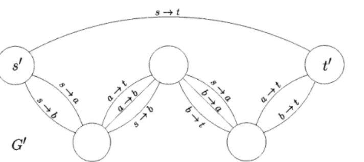
A monotone switching network solving directed connectivity on V(G) = {s, t, a, b} s -+ t

Figure 3-1: In this figure, we have a monotone switching network G' solving directed connectivity, i.e. there is a path from s' to t' in G' whose labels are consistent with the input graph G if and only if there is a path from s to t in G (where V(G) = {s, t, a, b}).

For example, if we have the edges s -* a, a -- b, and b -+ t in G, so there is a path

from s to t in G, then in G', starting from s', we can take the edge labeled s -+ a,

then the edge labeled a -+ b, then the edge labeled s -+ a, and finally the edge labeled b -+ t, and we will reach t'. On the other hand, if G has the edges s -+ a, a -+ b, b -+ a, and s -+ b and no other edges, so there is no path from s to t, then in G' there

(32)

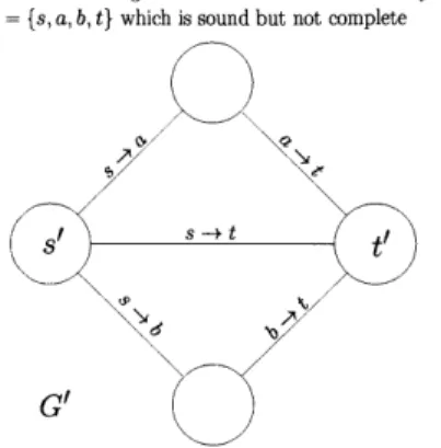
A monotone switching network for directed connectivity on

V(G) {s, a, b, t} which is sound but not complete

0,

G1

Figure 3-2: In this figure, we have another monotone switching network G'. This G' accepts the input graph G if and only G contains either the edge s -+ t, the edges

s -4 a and a - t, or the edges s -4 b and b - t. Thus, this G' is sound but not

complete.

Remark 3.1.5. Figures 3-2 and 3-3 illustrate why solving directed connectivity on a

set of vertices V(G) requires a larger switching network. Roughly speaking, the reason is that we are trying to simulate a directed graph with an undirected graph.

Remark 3.1.6. It is natural to ask where the examples of Figures 3-1 and 3-4 come

from. As we will see, there are many different ways to construct switching networks solving directed connectivity on a set of vertices and we will give the particular con-structions leading to the switching networks in Figures 3-1 and 3-4 later on. For now, the reader should just make sure that he/she understands Definition 3.1.1. That said, it is a good exercise to verify that these switching networks have the claimed properties and to try and figure out what they are doing.

In this thesis we analyze monotone switching networks. However, rather than looking at all possible input graphs, we focus on particular sets of input graphs. To do this, instead of assuming that the switching networks we analyze solve directed connectivity, we only assume that these switching networks solve the promise problem where the input graph G is guaranteed to either be in some set I of input graphs which contain a path from s to t or to not contain a path from s to t.

Definition 3.1.7. Given a set I of input graphs which all contain a path from s to t,

(33)

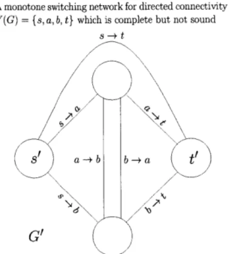
A monotone switching network for directed connectivity on

V(G) = {s, a, b, t} which is complete but not sound

8 a I -- + b b -- +a

G

Figure 3-3: In this figure, we have another monotone switching network G'. This G' accepts the input graph G whenever G contains a path from s -+ t (where V(G) =

{

s, t, a, b}), so it is complete. However, this G' is not sound. To see this, consider the input graph G with E(G) = {s -+ a, b -+ a, b -+ t}. In G', we can start at s', take

the edge labeled s - a, then the edge labeled b -+ a, then the edge labeled b -+ t, and we will reach t'. Thus, this G' accepts the given input graph G, but G does not contain a path from s to t because the edge from b to a goes the wrong way.

all of the input graphs in I.

In this chapter, we focus on input graphs which contain a path from s to t and no other edges, as they are the minimal YES instances and are thus the hardest input graphs for a monotone switching network to accept. We have the following definitions.

Definition 3.1.8. If V(G) is a set of vertices with distinguished vertices s, t,

1. Define PV(G),l to be the set of input graphs G such that E(G) = {vo - v1, vi

V2, * - - ,v1 _1 -+ v1} where v0 = s, vi = t, and vo, ,vi v.. are distinct vertices of V(G).

2. Define PV(G),<l = U j=1PV(G),j 3. Define PV(G) = 1 - PV(G),j

Proposition 3.1.9. A monotone switching network solves directed connectivity on

V(G) if and only if it is sound and accepts every input graph in

PV(G)-Corollary 3.1.10. The size of the smallest monotone switching network solving

(34)

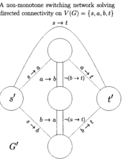
m(PV(G))-A non-monotone switching network solving directed connectivity on V(G) = {s, a, b, t}

b__'-( a t

t

G'

Figure 3-4: In this figure, we have a non-monotone switching network G' solving directed connectivity. Note that the edge with label -,(b - t) and the edge with label

-i(a -+ t) are necessary for G' to be complete. To see this, consider the input graph

G with E(G) = {s -+ a, a -+ b, b -+ t}. To get from s' to t' in G' we must first take

the edge labeled s -- a, then take the edge labeled a -- b, then take the edge labeled

-(a -+ t), and finally take the edge labeled b -÷ t.

In chapters 5 and 6 we will analyze the difficulty of directed connectivity for a given input graph G. To do this, we consider the promise problem where the input graph is guaranteed to either be isomormphic to G or to have no path from s to t.

Definition 3.1.11. Given an input graph G, let m(G) = m(I) where I = {G2 G2 is obtained from G by permuting the vertices of Vred(G)}

We give this definition here because it will make it easier for us to state some of the results of this chapter.

3.2 Certain Knowledge Switching Networks

In this section, we define certain knowledge switching networks, a subclass of sound monotone switching networks for directed connectivity which can be described by a simple reversible game for solving directed connectivity. We then prove upper

and lower bounds on the size of certain knowledge switching networks, showing that

certain-knowledge switching networks can match the performance of Savitch's algo-rithm and this is tight. The main result of this section is the following theorem.

(35)

Definition 3.2.1. Given a set I of input graphs all of which contain a path from s

to t, let c(I) be the size of the smallest certain-knowledge switching network which accepts all of the input graphs in I.

Theorem 3.2.2. Let V(G) be a set of vertices with distinguished vertices s, t. Taking

n Vre(G)J, if I > 2 and n > 2(l - 1) 2 then

1 n 1)_u ) F* 1 <- C(PV(G),1) <- C( V(G),<1) < nF11

2. -2 c(PV(G)) lgn+

3.2.1 The certain knowledge game for directed connectivity

We can use the following simple reversible game to determine whether there is a path from s to t in an input graph G.

Definition 3.2.3 (Certain knowledge game). We define a knowledge set K to be a

set of edges between vertices of V(G). An edge u -4 v in K represents the knowledge

that there is a path from u to v in G. We do not allow knowledge sets to contain

loops.

In the certain knowledge game, we start with the empty knowledge set K =

{}

and use the following types of moves:

1. If we directly see that v1 - v₂e E(G), we may add or remove v₁- v₂from K.

2. If edges v3 -+ v4, v4 -+ v5 are both in K and v3 -4 v5, we may add or remove V3 -+ v5 from K.

We win the certain knowledge game if we obtain a knowledge set K containing a path from s to t.

Proposition 3.2.4. The certain knowledge game is winnable for an input graph G if

(36)

3.2.2 Adapting the certain knowledge game for monotone

switch-ing networks

Intuitively, certain knowledge switching networks are switching networks G' where each vertex v' E V(G') corresponds to a knowledge set Kv, and the edges between the vertices of G' correspond to moves from one knowledge set to another. However, there are two issues that need to be addressed. First, if G' is a switching network,

I', v', w'

c

V(G'), and there are edges with label e between u' and v' and between v' and w', then we may as well add an edge with label e between u' and w'. This edge now represents not just one move in the game but rather several moves. Thus an edge in G' with label e should correspond to a sequence of moves from one knowledge set to another, each of which can be done with just the knowledge that e E E(G).

The second issue is that the basic certain knowledge game has many winning states but a switching network G' has only one accepting vertex t'. To address this, we need to merge all of the winning states of the game into one state. To do this, we add a move to the game allowing us to go from any winning state to any other winning state.

Definition 3.2.5 (Modified certain knowledge game). In the modified certain

knowl-edge game, we start with the empty knowlknowl-edge set K =

{}

_{and use the following types}

of moves:

1. If we directly see that v1 -+*v ₂E E(G), we may add or remove v₁- v₂from K.

2. If edges v3 -+ v₄, v₄ -+ v5 are both in K and v3 f v5, we may add or remove

v3 -+ v5 from K.

3. If s -4 t E K then we can add or remove any other edge from K.

We win the modified certain knowledge game if we obtain a knowledge set K containing a path from s to t.

Remark 3.2.6. In the modified certain knowledge game, an edge v1 .-+ v₂in K now

represents knowing that either there is a path from v1 to v2 in G or there is a path from s to t in G.

(37)

Proposition 3.2.7. The modified certain knowledge game is winnable for an input

graph G if and only if there is a path from s to t in G.

Definition 3.2.8. We say a monotone switching network G' is a certain knowledge

switching network if we can assign a knowledge set Kv, to each vertex v' G V(G') so that the following conditions hold:

1. Ks' =

{}

2. KtI contains a path from s to t (this may or may not be just the edge s - t)

3. If there is an edge with label e = v1 - v₂ between vertices v' and w' in G', then

we can go from Kv, to K&' with a sequence of moves in the modified certain knowledge game, all of which can be done using only the knowledge that v1

v2 c E(G).

We call such an assignment of knowledge sets to vertices of G' a certain knowledge description of G'.

Proposition 3.2.9. Every certain knowledge switching network is sound.

Proof. If there is a path from s' to t' in G' which is consistent with an input graph G then it corresponds to a sequence of moves in the modified certain knowledge game from K,, =

{}

to a K,, containing a path from s to t where each move can be done with an edge in G. This implies that the modified certain knowledge game can be won for the input graph G, so there is a path from s to t in G. D

3.2.3 A partial order on knowledge sets

There is a partial order on knowledge sets as follows. This allows us to restate the definition of certain knowledge switching networks more cleanly and will be important in Section 3.3

(38)

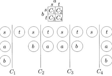
K={s a} s a a b an ' K=ese a, s - b}) _t K =} b b a _{K =Is -+} _tK b t K = -+ fs b}

Figure 3-5: In this figure, we have a certain knowledge switching network G' solv-ing directed connectivity (on V (G) = {s, t, a, b}) together with a certain knowledge description for it.

k. = {V1 -4 V2 : V1,V2 c V (G), v1 V2, there is a path

from

v1 to V2 whose edges are all in K} if s--4 t K

2. K = {vji V2 : V1, iV2 E V(G), vi V2} if s -+ t E K

Definition 3.2.11.

1. We say that K1 < K2 if K1 C K 2.

2. We say that K1 = K2 if K1 = K 2.

Remark 3.2.12. Intuitively, K describes all knowledge which can be deduced from

K. The statement that K1 < K2 means that all of the information that K1 represents about G is included in the information that K2 represents about G.

Proposition 3.2.13. If K1, K2, K3 are knowledge sets for V(G), then

1. K1 < K1 (reflexivity)

2. If K1 < K2 and K2 < K1 then K1 K2 (antisymmetry)

3. If K1 < K2 and K2 < K3 then K1 < K3 (transitivity)

(39)

1. For knowledge sets K1, K2, there is a sequence of moves from K1 to K2 in the modified certain knowledge game which does not require any information about the input graph G if and only if K1 K2.

2. For knowledge sets K1, K2 and a possible edge e of G, there is a sequence of

moves from K1 to K2 in the modified certain knowledge game which only requires the information that e E E(G) if and only if K1 U {e} 1 K2U {e}.

Corollary 3.2.15. We can restate the definition of certain knowledge switching

net-works as follows. A monotone switching network G' is a certain knowledge switching network if we can assign a knowledge set Kv, to each vertex v' e V(G') so that the

following conditions hold: 1. KSI =

{}

2. Kt, {s -+ t}

3. If there is an edge with label e = v1 - v₂ between vertices v' and w' in G', then

Kv, U {e} = Kw U {e}

3.2.4 Certain knowledge switching networks and reachability

from

s

While certain knowledge switching networks can consider all paths in G, most of our examples only consider reachability from s. For these examples, the following definition and lemma are extremely useful.

Definition 3.2.16. For each subset V C Vred(G), define Kv = {s - v : v E V}

Lemma 3.2.17. For any v1,v2 E Vred(G) and V C Vred(G) with v1 c V there is a sequence of moves in the modified certain knowledge game from Kv to Kvu{v2} which

only requires the knowledge that v1 -+ v2 G E(G)

Proof. Starting from K = Kv, take the following sequence of moves:

(40)

2. Add s -+ v2 to K (we already have s -- v, and vi -- v2 in K)

3. Remove v, - v₂from K.

We are now at K = KvuV{ 2} El

Remark 3.2.18. Note that there is no sequence of moves in the modified certain

knowledge game from Kvl to KIV2} which only requires the knowledge that v1 -+

V2 E E(G). The reason is that this is not reversible. We are forgetting the fact that

there is a path from s to v1 in G or a path from s to t in G and forgetting information

is irreversible. Also, while we can deduce that there is a path from s to v2 in G from the fact that there is a path from s to v1 in G and v1 -+ v2

e

E(G), we cannot deduce

that there is a path from s to v1 in G from the fact that there is a path from s to v2

in G and v1 v2 C E(G). s-t s b at Kja) Kf a,bj a t i s +b C t tl Kjbj Kfa,c) C t K{c)j K(b,c)

Figure 3-6: In this figure, we have a certain knowledge switching network G' solving directed connectivity (on V(G) = {s, t, a, b, c}) together with a certain-knowledge description for it. By default, we take K., =

{}

and Kt, = {s -+ t}.

Remark 3.2.19. Figure 3-6 shows how removing old information can help in finding

(41)

with V(G) = { s, t, a, b, c} and E(G) = {s -+ a, a -+ b, b -+ c, c -+ t}, then to get from s' to t' in G', we must first take the edge labeled s - a to reach K = K{a}, then take the edge labeled a -+ b to reach K = K{a,b}, then go "backwards" along the edge labeled s - a to reach K = K{b}, then take the edge labeled b -s c to reach K = K{b,,} and finally take the edge labeled c -+ t to reach t'.

3.2.5 An upper bound on certain-knowledge switching

net-works

While the certain knowledge condition is restrictive, certain knowledge switching networks nevertheless have considerable power. In particular, the following certain knowledge switching networks match the power of Savitch's algorithm.

Definition 3.2.20. Given a set of vertices V(G) with distinguished vertices s, t, let

G'(V(G), r) be the certain knowledge switching network with vertices t' U {v' : V C Vred(G), V|

<

r} and all labeled edges allowed by condition 3 of Definition 3.2.8,

where each v'v has knowledge set Kv, s' = v',, and K, =

{s

- t}.

Definition 3.2.21. Define G'(V(G)) = G'(V(G), n)

Example 3.2.22. The certain-knowledge switching network shown in Figure 3-5 is

G'({s, t, a, b}) = G'({ s, t, a, b}, 2). The certain-knowledge switching network shown in Figure 3-6 is G'({s, t, a, b, c}, 2).

Theorem 3.2.23. For all 1 > 1, c(Pv(G),<l) (f

()

+ 2

Proof. Consider the switching network G' = G'(V(G), [lg

11).

G' is a certain-knowledge switching network with IV(G') =

(n)

+2, so to prove the theorem it is sufficient

to show that G' accepts all of the input graphs in PV(G),<l.

Consider an input graph G -Pv(G),<l. E(G) = {vi -÷ vj : 0 < i <

J

- 1} where

vo = s', vj = t', and

j

< 1. We will show that G' accepts G by showing that we can win at the following reversible pebble game without placing more than [lg 1] pebbles on the vertices vi,. -, vj_1. This pebble game was introduced by Bennet

[3

to study time/space tradeoffs in computation.

Analyzing monotone space complexity via the switching network model

Analyzing Monotone Space Complexity Via the

Switching Network Model

by

Aaron H. Potechin

Submitted to the Department of Mathematics

ARCHIVES

JUN 3

0

2015

LIBRARIES

in partial fulfillment of the requirements for the degree of

Doctor of Philosophy in Mathematics

at the

MASSACHUSETTS INSTITUTE OF TECHNOLOGY

June 2015

Massachusetts Institute of Technology 2015. All rights reserved.

Signature redacted

Department of Mathematics

May 8, 2015

Certified by...

Signature

redacted-Jonathan A. Kelner

Associate Professor

Thesis Supervisor

Accepted by ...

Signature redacted

Wichel X. Goemans

Analyzing Monotone Space Complexity Via the Switching

Network Model

by

Aaron H. Potechin

Abstract

Acknowledgments

Contents

List of Figures

Chapter 1

Introduction

1.1

Known Results on Space Complexity

1.2

Approaches to Space Lower Bounds

[7]

[16]

1.3

Known Results on Monotone Complexity

[

#

#

1.4

Overview of Our Results

Chapter 2

Background Material

|V(G')|,

{0,

{0,

2.1

Switching Networks: From Practice to Theory

f =

2.2

Turing machines and space complexity

Q

Q

Q

4.

Q

Q

Q

{L,

f

4.

{0,

c

2.3

Switching-and-rectifier networks and

nondeter-ministic space complexity

|V(G)

{0,1}"

{0,

c

_Q