Wireless Passive Sensors Interrogation Technique Based on a Three-Dimensional Analysis

HAL Id: hal-01396848

https://hal.archives-ouvertes.fr/hal-01396848

Submitted on 15 Nov 2016

HAL is a multi-disciplinary open access

archive for the deposit and dissemination of

sci-entific research documents, whether they are

pub-lished or not. The documents may come from

teaching and research institutions in France or

abroad, or from public or private research centers.

L’archive ouverte pluridisciplinaire HAL, est

destinée au dépôt et à la diffusion de documents

scientifiques de niveau recherche, publiés ou non,

émanant des établissements d’enseignement et de

recherche français ou étrangers, des laboratoires

publics ou privés.

Wireless Passive Sensors Interrogation Technique Based

on a Three-Dimensional Analysis

Dominique Henry, Hervé Aubert, Patrick Pons

To cite this version:

Dominique Henry, Hervé Aubert, Patrick Pons. Wireless Passive Sensors Interrogation Technique

Based on a Three-Dimensional Analysis. European Microwave Week (EuMW), Oct 2016, London,

United Kingdom. �hal-01396848�

Wireless Passive Sensors Interrogation Technique

Based on a Three-Dimensional Analysis

D.Henry, H.Aubert and P.Pons

LAAS-CNRS ; 7 av. du colonel Roche

31077 Toulouse, France

University of Toulouse; INP; F-31077 Toulouse, France [email protected], [email protected], [email protected]

Abstract—This paper describes a novel wireless passive

sensors interrogation technique based on a three-dimensional analysis. Variable impedances acting as passive sensors are remotely read by a 24 GHz bistatic FMCW radar at distances of 2.0 meters and 5.5 meters. The radar performs a mechanical beam scanning to receive the electromagnetic echo level response in a volume. Several estimators are compared to calibrate and quantify the passive sensor input impedance. From this impedance the physical quantity of interest (temperature, pressure, strain …) can be derived.

Keywords— wireless passive sensors, 3D radar imaging, remote sensing, isosurfaces.

I. INTRODUCTION

The wireless interrogation of passive sensors (tags without batteries and integrated circuits) is challenging. Many applications require autonomous sensors with a long life-time able to measure various physical quantities such as temperature, pressure or moisture. However these sensors must achieve good performances in terms of distance of interrogation, size, resolution, sensitivity and full-scale measurement range. Radio Frequency IDentification (RFID) is the most commonly used technology for passive sensing. Sensing elements can be easily integrated in RFID tags but the distance of interrogation is limited to few meters due to power regulations. Surface Acoustic Wave (SAW) sensors are also investigated but their operating frequency is limited to few GHz. Harmonic (or intermodulation) radars can remotely read tags with a good achievable range. Nevertheless their different carrier frequencies at transmission and reception do not fit with radio regulations.

A novel passive sensor interrogation technique based on a three-dimensional scanning has been recently reported by the authors in [1]. A Frequency-Modulated Continuous-Wave (FMCW) radar operating at 24 GHz was used for the detection and localization of the sensors and for deriving the variation of sensors input impedance from standard algorithms and signal processing techniques applied to 3D radar images [1][2]. From this impedance the physical quantity of interest (temperature, pressure, strain …) can be deduced. The present paper compares the performances of several possible estimators for the remote derivation of passive sensors input impedance from the three-dimensional analysis of radar images.

Section II describes the beam scanning radar system and the interrogated passive sensors. Section III defines various

possible estimators for deriving the input impedance of the sensors from the 3D analysis of radar images. The impedance variation is finally displayed in three dimensions using iso-surfaces.

II. 3DBEAM SCANNING TECHNIQUE

A. Reader system

The reader is a bistatic FMCW radar transmitting a chirp at a carrier frequency fc = 23.8 GHz and frequency modulated with a triangular signal. This signal has a ramp-time T = 1 ms and a frequency bandwidth B = 2 GHz. The standard definition of the theoretical depth resolution d is the given by [3]:

B

c

d





2

(1)

where c is the celerity of light in air. In our configuration, a theoretical depth resolution of 7.5 cm can be reached. Different antennas are used for transmission and reception purposes. A parabolic antenna is connected to the front-end of the Tx channel. It has a gain of 33.5 dBi and a beamwitdh of 2°. Knowing that the input power of the radar is 10.8 dBm, the EIRP is 44.3 dBm. The reception antenna is a 1x5 patches array with a gain of 8.6dBi and a beamwitdh of 80° in azimuth and 20° in elevation. The radar and its antennas are mounted on a pan-tilt platform automatically controlled by a computer unit (Figure 1). It performs a 3D spherical scanning from θMin = -10° to θMax = 10° in azimuth with a step Δθ = 2° and φMin = -10° to

φMax = 10° in elevation with a step Δφ = 2°. For each step, a chirp is transmitted. The signal backscattered by the scene is then demodulated and filtered by the radar.

The passive sensor is composed of three parts : (a) a horn antenna of gain 20 dBi and a 60° beamwidth, (b) a coaxial cable with an effective length of L = 1.35m (delay line) and (c) a variable attenuator terminated with a short-circuit. The measurement principle is based on load scatterers theory [4]. The structural mode is used to localize the sensor, and the sensing (or antenna) mode is analyze to derive the input impedance of the sensor and consequently, to deduce the physical quantity of interest. The variation of the sensor input impedance is simulated here from the tuning of an attenuator.

B. Data acquisition and signal processing

For each sweep step we perform an averaging of 10 time

signals. I and Q signals of the reception channel are used in order to compute the complex signal. The time signal is digitalized into 1024 samples and normalized with the maximal voltage of the ADC (3.3V). A back-projection algorithm is applied to determine the echo level for each cell that has been scanned [5]. The rotating beam scanning generates resolution cells in spherical coordinates. The volume

VSpher of such resolution cell is then given as follows:

_                                  2 sin 2 2 3 2 3 d 3 _  R d R V_Spher (2)

where R denotes to the distance from the center of the resolution cell to the radar. The cell volume grows with the distance of interrogation. A transformation to Cartesian coordinates is applied with a spline interpolation for increasing the resolution and for facilitating the analysis of 3D radar image. The new volume VCart of resolution cell and the Cartesian grid are defined such as:

V

_Cart





x





y





z

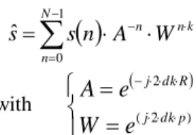
(3) with                                p d p B c z p R y p R x y Min x Min 2 2 tan 2 2 tan 2   (4)

where RMin and RMax designate the minimal and maximal ranges in which the Cartesian transformation operates. The parameters px and py are increasing resolution factors of x and y cross-range axes. The parameter p is a pad factor which represents a zoom range performed by the chirp-z transformation defines as follows [6]

 

n nk N n W A n s s       



1 0 ˆ (5) with  











       ) 2 ( 2 p dk j R dk j

e

W

e

A

(6) In Eq.(5)

sˆ

denotes the result of the chirp-z transformation of the sampled time signal s and N is the total number of samples. In Eq.(6) R designates the distance from the resolution cell to the radar and dk is the wave number increment. The dimensions of the 3D Cartesian grid (XMin,

XMax), (YMin, YMax) and (ZMin, ZMax) are given by:



_

_



_



_



_



_



_



_







            _{ }    2 2 2 , , tan , tan , tan , tan , Max Max Max Min Max Min Max Min Min Min Max Min Max Min Min Min Max Min Y X R R Z Z R R Y Y R R X X     (7)

The Fig. 2 illustrates the Cartesian transformation Eqs. (3)-(6). The final step consists of displaying the data in three dimensions. This can be achieved with the help of isosurfaces given a representation of each layer of equal echo level (see section III).

III. MEASUREMENT RESULTS AND DISCUSSION

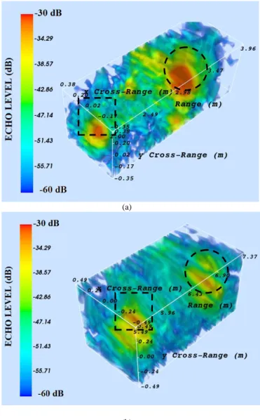
Measurements are performed for different values of sensor impedances when the passive sensor is placed at a distance of 2 meters (scenario I) or 5.5 meters (scenario II) from the reader. Fig 2 shows the resulting 3D isosurfaces display for a sensor impedance of 0Ω. Structural and sensing modes are clearly detectable and separated by the coaxial cable effective length (1.35 meters). In such isosurfaces echo levels having the same amplitudes are assigned to a specific colored layer. The transparency of each layer increases when the amplitude of the radar echo decreases. This visualization based on isosurfaces is a great tool for displaying a global volume and for roughly observing the 3D distribution of radar echo levels. When the sensing mode is localized, a volume of study is defined around the corresponding radar echo level. This

Fig 2. Scanning grid in spherical coordinates and its corresponding Cartesian grid after Cartesian transformation Eqs. (3)-(6) for a given

elevation cut-plane Fig 1. Measurement system and passive sensor located at

volume is defined in Table I. For the two above-mentioned scenarios, this volume is composed of several resolution cells, respectively 32832 cells (scenario I) or 23598 cells (scenario II). The volume is of 0.29 m3 (scenario I) and of 0.21 m3 (scenario II). Consequently the beam scanning analysis does not only focus on a single value of the magnitude, but on several values distributed in a three-dimensional space. This approach allows the definition of several estimators. These estimators may provide a direct relationship between the value of the sensor input impedance value and the magnitude variation of the sensing mode in a volume.

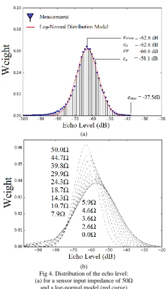
Fig.4.a shows the distribution of the echo level for a sensor input impedance of 50 Ω. By choosing a volume containing a sufficient number of resolution cells, the distribution tends to a log-normal distribution given by:

 

           _   2 2 2 ln 2  







x e x K x (8) where K and σ are scale factors and µ is the location factor. Each black bar corresponds to the weight of cells in which the echo level ranges between two extreme values defined by an echo level step (a step of 1dB is chosen here for illustration purpose). The red curve is plotted by using a curve fitting algorithm with a cubic interpolation of 1000 points and parameters of the log-normal distribution in equation (8) are extracted.

Fig.4.b shows that the shape of the log-normal distribution changes with the sensor input impedance. Hence it is possible to define estimators which depend directly from the log-normal distribution parameters. In order to estimate the variation of the echo level, five estimators are compared:

(a) eMax is the maximal value of the measured echo level. Hence it concerns only one resolution cell. This is the most instinctive estimator;

(b) eA is the mean echo level in the entire volume. It considers every echo level values of cells with the same weight;

(c) eW represents the weighted arithmetic mean of the distributed echo level given by:



 





1 0 M n n n W

W

P

e

(9) where Pn corresponds to a sliding threshold, Wn the percentage number of cells for which magnitude A is such as

Pn+1≥A≥Pn, M is an integer such as PM = 0 dB (or the maximal reachable value of echo level). As mentioned before, the echo level step is Pn+1-Pn = 1dB. Cells with higher values are assigned to higher weights;

(d) eµ is the location parameter of the log-normal distribution. It is defined such as:

eµexp

 

µ (10)

It represents the shift of the log-normal distribution;

(e) emode is the mode (maximum point or value of the peak) of the log-normal distribution. It is defined as:



2



mod expµ

e _e (11) Value indicators of these estimators are plotted on Fig.4.a.

(a)

(b)

Fig 3. Structural (square) and sensing (circle) modes representation with isosurfaces for a sensor position at (a) 2m and (b) 5.5m.

TABLEI

SENSING MODE VOLUME CHARACTERISTICS

Scenario I Scenario II Minimal range RMin 3.20 m 6.84 m

Maximal range RMax 4.00 m 7.18 m

x-resolution scale factor px 3.2 6.84 y-resolution scale factor py 3.2 6.84 Pad factor p 10 10 x-axis resolution Δx 3.5 cm 3.5 cm y-axis resolution Δy 3.5 cm 3.5 cm z-axis resolution Δz 7.5 mm 7.5 mm x cross-range size [XMin

-XMax]

[-31 cm, 31 cm]

[-59 cm, 31 cm] y cross-range size [YMin

-YMax]

[-38 cm, 21 cm]

[-31 cm, 31 cm] Resolution cell volume VCart 9 cm3 9 cm3

Estimators are plotted on Fig.5 for the scenario I and scenario II. The estimator eMax has the best performances in terms of the full-scale measurement range (17.1dB and 15.6dB) with a good sensitivity (>-0.4dB/ Ω). However there is minimal threshold starting from 40 Ω where the sensor impedance cannot be estimated. That is why the four other estimators are helpful: they take into account the magnitude fluctuation of surrounding cells. Best results are obtained with the estimator eµ (location parameter of the log-normal distribution). It has full-scale measurement range of 16.5 dB at 2.0 m and 10.8 dB at 5.5 m with a sensitivity of -0.3dB/Ω. Moreover, it has a linear behavior with a correlation coefficient R² > 0.990.

IV. CONCLUSION

A novel scanning technique has been described in order to remotely read passive sensors. After a brief explanation of the Cartesian grid construction, a display with isosurfaces allows a representation of structural and sensing modes in 3D radar images. Then a study on a specific volume centered on the sensing mode is applied for two sensors positions (2.0m and 5.5m) and for various sensor impedances (from 0 Ω to 50 Ω). It is observed that the echo level distribution can be modeled as a

log-normal distribution and specific estimators are defined to derive the sensor impedance variation for radar images. Estimators that take into account several resolution cells show better results in linearity than one (more intuitive) which considers only the value of the maximal echo level.

REFERENCES

[1] Henry, D.; Pons, P.; Aubert, H., "3D scanning radar for the remote reading of passive electromagnetic sensors," in Microwave Symposium

(IMS), 2015 IEEE MTT-S International , pp.1-4, 17-22 May 2015

[2] Henry, D.; Pons, P.; Aubert, H., "3D microwave imaging system for the remote detection and reading of passive sensors," in Microwave

Conference (EuMC), 2015 European , pp.259-262, 7-10 Sept. 2015.

[3] S.O. Piper, "Receiver frequency resolution for range resolution in homodyne FMCW radar," Telesystems Conference: Commercial

Applications and Dual-Use Technology, 16-17 June 1993, pp.169-173

[4] Harrington, Roger F., "Theory of loaded scatterers," Proceedings of the Institution of Electrical Engineers, vol.111, no.4, pp.617-623, April 1964 [5] Haderer, A.; Scherz, P.; Schrattenecker, J.; Stelzer, A., "Real-time implementation of an FMCW backprojection algorithm for 1D and 2D apertures," in Radar Conference (EuRAD), 2011 European , pp.53-56, 12-14 Oct. 2011.

[6] Rabiner, L.; Schafer, R.W.; Rader, C.M., "The chirp z-transform algorithm," in IEEE Transactions on Audio and Electroacoustics, vol.17, no.2, pp.86-92, Jun 1969

(a)

(b)

Fig 5. Echo Level vs. the sensor input resistance using the 5 studied estimators at (a) 2.0m and (b) 5.5m

(a)

(b)

Fig 4. Distribution of the echo level: (a) for a sensor input impedance of 50Ω

and a log-normal model (red curve)