Extracting linked data from statistic spreadsheets

HAL Id: hal-01583975

https://hal.inria.fr/hal-01583975

Submitted on 8 Sep 2017

HAL is a multi-disciplinary open access

archive for the deposit and dissemination of

sci-entific research documents, whether they are

pub-lished or not. The documents may come from

teaching and research institutions in France or

abroad, or from public or private research centers.

L’archive ouverte pluridisciplinaire HAL, est

destinée au dépôt et à la diffusion de documents

scientifiques de niveau recherche, publiés ou non,

émanant des établissements d’enseignement et de

recherche français ou étrangers, des laboratoires

publics ou privés.

Extracting linked data from statistic spreadsheets

Tien Duc Cao, Ioana Manolescu, Xavier Tannier

To cite this version:

Tien Duc Cao, Ioana Manolescu, Xavier Tannier. Extracting linked data from statistic

spreadsheets. International Workshop on Semantic Big Data, May 2017, Chicago, United States. pp.1

-5, �10.1145/3066911.3066914�. �hal-01583975�

Tien Duc Cao

Ioana Manolescu

Xavier Tannier

LIMSI, CNRS, Univ. Paris-Sud, Universit´e Paris-Saclay xavier.tannier@limsi.fr

ABSTRACT

Statistic data is an important sub-category of open data; it is in-teresting for many applications, including but not limited to data journalism, as such data is typically of high quality, and reflects (under an aggregated form) important aspects of a society’s life such as births, immigration, economic output etc. However, such open data is often not published as Linked Open Data (LOD) limiting its usability.

We provide a conceptual model for the open data comprised in statistic files published by INSEE, the leading French economic and societal statistics institute. Then, we describe a novel method for extracting RDF LOD populating an instance of this conceptual model. Our method was used to produce RDF data out of 20k+ Excel spreadsheets, and our validation indicates a 91% rate of successful extraction.

KEYWORDS

Linked Data, Information Extraction, RDF

1

INTRODUCTION

The tremendous value of Big Data has been noticed of late also by the media, and the term “data journalism” has been coined to refer to journalistic work inspired by data sources [6]. While data of some form is a natural ingredient of all reporting, the increasing volumes of available digital data as well as its increasing complexity lead to a qualitative jump, where technical skills for working with data are stringently needed in journalism teams.

A class of data sources of particularly high value is that com-prised into government statistics. Such data has been painstakingly collected by state administrations which sometimes have very sig-nificant human and technology means at their disposal, especially in countries like France with an old history of statistics gathering1. This makes the data oftentimes of high quality. Another important quality of such government statistic data is that it logically falls into the open data category, since it is paid for with taxpayer money.

Such high-quality statistic data is a very good background in-formation to be used when trying to assess the truthfulness of a claim. A general description of a fact-checking scenario can be constructed as follows: first, a claim is made. Second, journalists or other fact-checkers look up reference sources providing relevant sta-tistics for the assessment of the claim; Third, some post-processing may need to be applied to compute from the reference source values, the value corresponding to the claim. This post-processing may involve elaborate steps.

1_{In France, this started with Jean-Baptiste Colbert (1619-1683), the acclaimed finance}

minister of king Louis XIV).

In this work, we focus on the extraction of reference sources. In the best-case scenario, reference data sources are available to fact-checkers in a format and organized according to a model that they understand well. For instance, in [11], unemployment data is assumed available in a temporal database relation. This assumption is very reasonable for statisticians and other scientists working within the statistics institutes. However, unfortunately, most fact-checking actors are outside these institutes, and only have access to the data through publication by the institute. This raises the question of the format and organization of the data. While the W3C’s best practices argue for the usage of RDF in publishing open data [10], in practice open data is often published in other formats, such as Excel, HTML or PDF; in the latter formats, statistic data is typically shown as tables or charts. In the particular case of the INSEE2, the leading French social and economic statistics institute, while searching for some hot topics in the current French political debate (youth unemployment, immigrant population etc.) we found many very useful datasets, available as Excel and/or HTML and sometimes accompanied by a PDF report explaining and commenting the data, but we did not find the data in a structured, machine-readable format.

Motivated by this limitation, we propose an approach for extract-ing Linked Open Data from INSEE Excel tables. The two main contributions of our work are: (i) a conceptual data model (and con-crete RDF implementation) for statistic data such as published by INSEE and other similar institutions, and (ii) an extraction algorithm which populates this model based on about11,000 pages including 20,743 Excel files published by INSEE.

Below, we describe the data sources we work with and the model for the extracted data (Section 2) and our extraction method (Sec-tion 3), outline the format of the extracted RDF data (Sec(Sec-tion 4), and present an evaluation of our extraction process (Section 5), before discussing related work and concluding.

2_{INSEE: French National Institute of Statistics and Economic Studies,}

, , Tien Duc Cao, Ioana Manolescu, and Xavier Tannier H H H H_H l c 1 2 3 4 5 6 7 8 9 10

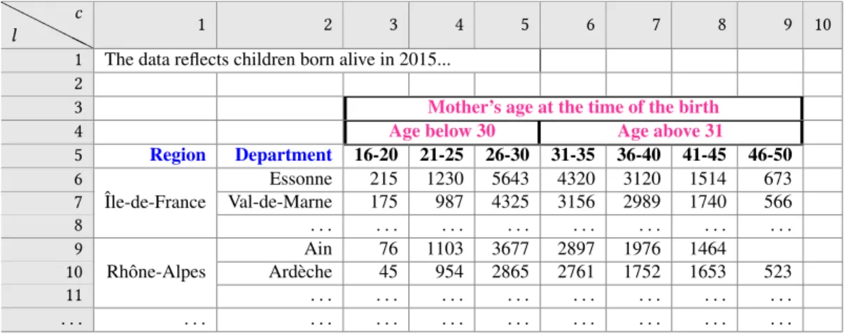
1 The data reflects children born alive in 2015... 2

3 Mother’s age at the time of the birth

4 Age below 30 Age above 31

5 Region Department 16-20 21-25 26-30 31-35 36-40 41-45 46-50 6 ˆIle-de-France Essonne 215 1230 5643 4320 3120 1514 673 7 Val-de-Marne 175 987 4325 3156 2989 1740 566 8 . . . . 9 Rhˆone-Alpes Ain 76 1103 3677 2897 1976 1464 10 Ard`eche 45 954 2865 2761 1752 1653 523 11 . . . . . . . .

Figure 1: Outline of a sample statistics table in an INSEE dataset.

2

REFERENCE STATISTIC DATA

In Section 2.1, we present the input INSEE statistics, while Sec-tion 2.2 describes our conceptual model for this data.

2.1

INSEE data sources

INSEE publishes a variety of datasets in many different formats. In particular, we performed a crawl of the INSEE web site under the categories Data/Key figures, Data/Detailed figures, Data/Databases, and Publications/Wide-audience publications, which has lead to about11,000 web pages including 20,743 Excel files (with total size of 36GB) and20,116 HTML tables. In this work, we focused on the set of Excel files; we believe our techniques could be quite easily adapted to HTML tables in the future. Also, while we targeted INSEE in this work, we found similar-structure files published in other Open Data government servers in the UK3and the US4. Thus, we believe our tool can be used to handle more than the data sources we considered so far.

We view each spreadsheet file as a collection of data sheets D1,D2, . . . Each data sheet D has a title D.t and optionally an outline

D.o. The title and outline are given by the statisticians producing the spreadsheets in order to facilitate their understanding by human users, such as the media and general public. The title is a short nominal phrase stating whatD contains, e.g., “Average mothers’ age at the birth of their child per department in 2015”. The outline, when present, is a short paragraph which may be found on a Web page from where the file enclosingD can be downloaded. The outline extends the title, for instance to state that the mothers’ ages are rounded to the closest smaller integers, that only the births of live (not stillborn) children are accounted for etc.

In a majority of cases (about two thirds in our estimation), each data sheetD comprises one statistics table, which is typically a two-dimensional aggregate table. Data is aggregated since statistics institutes such as INSEE are concerned with building such global measures of society or economy phenomena, and the aggregate tends to be bidimensional since they are meant to be laid out in a 3_{E.g., http://www.ic.nhs.uk/catalogue/PUB08694/ifs-uk-2010-chap1-tab.xls.} 4_{E.g., http://www.eia.gov/totalenergy/data/monthly/query/mer data excel.asp?}

table=T02.01.

format easy for humans to read. For instance, Figure 1 illustrates a data sheet for the birth statistic dataset mentioned above. In this example, the two dimensions are the mother’s age interval, e.g., “16-20”, “21-25”, “26-30” etc. and her geographic area, specified as a department, e.g., “Essonne”, “Val-de-Marne” etc. For a given age interval and region, the table includes the number of women which were first-time mothers in France in 2015, in that age interval and department. In Figure 1, we have included a top row and column on a gray background, in order to refer to the row and column numbers of the cells in the sheet. We will use the shorthandDr,cto denote the

cell at rowr and column c in D. We see that the table contains data cells, such asD6,3,D6,4, which hold data values, etc. and header

cells, e.g., “Region”, “Age below 30” etc., which (i) characterize (provide context for) the data values, and (ii) may occupy several cells in the spreadsheet, as is the case of the latter.

The basic kind of two-dimensional agregate in a data sheet is (close to) the result of a group-by query, as illustrated in Figure 1. However, we also found cases where the data sheet contains a data cube[7], that is: the result of a group-by, enhanced with partial sums along some of the group-by dimensions. For instance, in the above example, the table may contain a row for every region labeled “Region total” which sums up the numbers for all departments of the

region, for each age interval5

Dimension hierarchiesare often present in the data. For instance, the dimension values “16-20”, “21-25”, “26-30” are shown in Fig-ure 1 as subdivisions of “Age below 30”, while the next four intervals may be presented as part of “Age above 31”. The age dimension hierarchy is shown in magenta in Figure 1, while the geographical dimension hierarchy is shown in blue. In those cases, the lower-granularity dimension values appear in the table close close to the finer-granularity dimension values which they aggregate, as exem-plified in Figure 1. Cell fusion is used in this case to give a visual cue of the finer-granularity dimension values corresponding to the lower-granularity dimension value which aggregates them.

A few more rules govern data organization in the spreadsheet:

5_{A sample real-life file from INSEE illustrating such cube tables is:}

https://www.insee.fr/fr/statistiques/fichier/2383936/ARA CD 2016 action sociale 1-Population selon l age.xls.

• D1,1(and in some cases, more cells on row1, or the first few

rows ofD) contain the outline D.o, as illustrated in Figure 1; here, the outline is a long text, thus a spreadsheet editor would typically show it overflowing over several cells. One or several fully empty rows separate the outline from the topmost cells of the data table; in our example, this is the case of row2. Observe that due to the way data is spatially laid out in the sheet, these topmost cells are related to the lowest granularity (top of the hierarchy) of one dimension of the aggregate. For instance, in Figure 1, this concerns the cell at line3 and columns 3 to 9, containingMother’s age at the time of the birth.

• Sometimes, the content of a header cell (that is, a value of an aggregation dimension) is not immediately understand-able by humans, but it is the name of a variunderstand-able or measure, consistently used in all INSEE publications to refer to a given concept. Exactly in these cases, the file containing D has a sheet immediately after D, where the variable (or measure) name is mapped to the natural-language descrip-tion explaining its meaning. For example, we translate

SEXE1 AGEPYR10186into Male from 18 to 24 years old.

Variable Meaning

SEXE Sex

1 Male

2 Female

AGEPYR10 Age group

00 Less than 3 years old

03 3 to 5 years old 06 6 to 10 years old 11 11 to 17 years old 18 18 to 24 years old 25 25 to 39 years old . . . . 80 80 years old

2.2

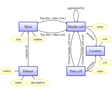
Conceptual data model

From the above description of the INSEE statistic datasets, we extract a conceptual data model shown in Figure 2. Entities are shown as boxes while attributes apper in oval shapes. We simplified the notation to depict relationships as directed arrows, labeled with the relationship name. Data cells and header cells each have an attribute indicating their value (content); by definition, any data or header cell has a non-empty content. Moreover, a data cell has one associated location, i.e., (row number, column number), while a header cell may occupy one or several (adjacent) locations. Each data cell has a closest header cell on its column, and another one on its line; these capture the dimension values corresponding to a data cell. For instance, the closest column header cell for the data cell atD7,4 isD5,4, while the closest column header cell isD7,2.

Further, the header cells are organized in an aggregation hierarchy materialized by the respective relation “aggregated by”. For instance, D5,4 is aggregated byD4,3, which is agregated byD3,3. In each

sheet, we identify the top dimension values as those which are not aggregated by any other values: in our example, the top dimension values appear inD3,3,D6,1andD9,1. Note that such top dimension

values are sometimes dimensions names, e.g.,Region, and other 6_{https://www.insee.fr/fr/statistiques/fichier/2045005/BTX TD POP1A 2013.zip}

Data cell value Header cell value

Closest header cell (ro w) Closest header cell (col) aggregated by Location row col position position Sheet title outline

Top dim. value (row)

Top dim. value (col)

Dataset

name description source

consists

of

Figure 2: Conceptual data model.

times dimensions values, e.g., ˆIle-de-France. Indeed, statistics in a sheet are not guaranteed to be organized exactly as predicted by the formal models of relational aggregation queries, even if they typically come very close.

Finally, note that our current data model does not account for data cubes, that is: we do not model the cases when some data cells are aggregations over the values of other data cells. Thus, our current extraction algorithm (described below) would extract data from such cubes as if they were result of a plain aggregation query. This clearly introduces some loss of information; we are working to improve it in a future version.

3

EXTRACTION

We developed a tool for extracting data from spreadsheet files so as to populate an instance of our conceptual data model; it uses the Python library xlrd7for accessing spreadsheet content. Below, we present the extraction procedure. Unlike related work (see Section 6), it is not based on a sequence classification with a supervised learning approach, but on a more global rule-based system aiming at framing the data cell range and extracting the headers around these data cell.

For each sheet, the first task is to identify the data cells. In our cor-pus, these cells contain numeric information, that is: integers or real numbers, but also interval specifications such as “20+” (standing for “at least 20”), special null tokens such as “n.s.” for “not specified”. Our approach is to identify the rectangular area containing the main table (of data cells), then build data cells out of the (row, column) locations found in this area. Note that the area may also contain empty locations, corresponding to the real-life situation when an information is not available or for some reason not reported, as is the case forD9,9in Figure 1.

Data cell identification proceeds in several steps.

(1) Identify the leftmost data location (ldl) on each row: this is the first location encountered from left to right which 7_{https://pypi.python.org/pypi/xlrd}

, , Tien Duc Cao, Ioana Manolescu, and Xavier Tannier (i) follows at least one location containing text (such

loca-tions will be interpreted as being part of header cells), and (ii) has a non-empty content that is compatible with a data cell (as specified above). We store the column numbers of all such leftmost data locations in an array calledldl; for instance,ldl[1] = −1 (no data cell detected on row 1) and the same holds for rows2 to 5, whileldl[i] = 3 for i = 6,7 etc.

(2) For each rowi where ldl[i] , −1, we compute a row signa-turesiд[i] which is counts the non-empty locations of vari-ous types found on the row. For instance,siд[6] = {strinд : 2,num : 7} because the row has 2 string-valued cells (“ˆIle-de-France” and “Essonne”) and7 numerical cells. For each signature thus obtained, we count the number of rows (with data cells) having exactly that signature; the largest row set is termed the data table seed. Note that the rows in the data table seed are not necessarily contiguous. This reflects the observation that slightly different-structured rows are sometimes found within the data table; for instance,D9,9

is empty, therefore row9 is not part of the seed, which in this example, consists of the rows {6,7,8,10,11} and possibly other rows (not shown) below.

(3) We “grow” the data table seed it by adding every row at distance 1 or at most 2 above and below the data table seed, and which contains at least a data cell. We do this repeatedly until no such rows can be found. In our example, this process adds row9, despite the fact that it does not have the same signature as the others. We repeat this step in an inflationary fashion until no row adjacent to the current data table qualifies. The goal of this stage is to make sure we do not miss interesting data cells by being overly strict w.r.t. the structure of the rows containing data cells. At this point, all the data cells are known, and their values and coordinates can be extracted.

Identification and extraction of header cells We first look for those organized in rows, e.g., rows3, 4 and 5 in our example.

(1) We attempt to exploit the visual layout of the file, by look-ing for a horizontal border which separates the first header row of the (usually empty) row above it.

(a) When such a border exists (which represents a major-ity but not all the cases), it is a good indicator that header cells are to be found in the rows between the border and going down until (and before) the first data row. (Note that the data rows are already known by now.) In our example, this corresponds to the rectan-gular area whose corners areD3,1andD4,9.

(b) When the border does not exist, we look at the row immediately above the first data row, and then move up row by row to the top of the sheet; in each row i, we examine the locations starting at the column ldl[i] (if this is greater than 0). If the row doesn’t contain empty locations, we consider that it is part of the header area. Intuitively, this is because no data cell can lack a value along one of the dimensions, and header cells carry exactly dimension values. An

empty header cell would correspond precisely to such a missing dimension value.

(2) Once the header area is known, we look for conceptual header cells. The task is complicated by the fact that such a cell may be spread over several locations: typically, a short text is spread from the top to the bottom over locations situ-ated one on top of the other. This can also happen between locations in the same row (not in the same column), which are fused: this is the case ofD3,3toD3,9in our example.

The locations holding a single dimension value are some-times (but not always) fused in the spreadsheet; somesome-times, empty locations are enclosed within the same border as some locations holding text, to obtain a visually pleasing aspect where the dimension value “stands out well”. We de-tect such groups by tracking visible cell borders, and create one conceptual header cell out of each area border-enclosed area8.

Next, we identify and extract header cells organized in columns, e.g., columns1 and 2 in our example. This is done by traversing all the data rows in the data area, and collecting from each rowi, the cells that are at the left of the leftmost data cellldl[i].

Finally, we populate the instance of the data model with the re-maining relationships we need: we connect each data and header cell to its respective locations; we connect each data cell with its closest header cell on the same column, and with its closest header cell on the same row; and we connect each row (respectively, col-umn) header cell to its closest header cell above (respectively, at left) through the relation aggregated by.

4

LINKED DATA VOCABULARY

To represent the extracted data in RDF, we created an RDF class for each entity, and assigned an URI to each entity instance; the properties and their typing follow directly from the entity attributes and relationships shown in Figure 2.

Some sample triples resulting from the extraction are shown in Figure 3. We use the namespace inseeXtr.excel: for classes and properties we introduce in our extraction from INSEE Excel tables, and the namespace rdf: to denote the standard namespace associated to the W3C’s type property. The snippet in Figure 3 corresponds to one Excel file, one sheet in the file, a row header cell, a column header cell, a data cell associated to them, and the location of the data cell.

8_{The reader may wonder at this point: if a horizontal border on top of the header row is}

absent, how can one detect multi-location header cells by following borders? This case has never turned out in the files we examined, which is reasonable if we consider the hard-to-interpret visual aspect it would lead to. Thus, in our experience, when the top border is absent, each row header cell occupies only one location.

¡http://inseeXtr.excel:File0¿

rdf:type ¡http://inseeXtr.excel:Dataset¿;

inseeXtr:source ”http://insee.fr/.../Age M`ere ....xls”; inseeXtr:name ”Age M`ere ....xls”;

inseeXtr:description ”The data reflects children...” . ¡http://inseeXtr.excel:Sheet0¿

rdf:type ¡http://inseeXtr.excel:Sheet¿; inseeXtr:title ”sheet title”;

inseeXtr:belongsTo ¡http://inseeXtr.excel:File0¿ . ¡http://inseeXtr.excel:HeaderCellY0¿ inseeXtr:value ”x1”;

rdf:type ¡http://inseeXtr.excel:HeaderCellY¿; inseeXtr:YHierarchy ¡http://inseeXtr.excel:Sheet0¿ . ¡http://inseeXtr.excel:HeaderCellX2¿ inseeXtr:value ”a1”;

rdf:type ¡http://inseeXtr.excel:HeaderCellX¿; inseeXtr:aggregatedBy ¡http://inseeXtr.excel:HeaderCellX3¿; inseeXtr:XHierarchy ¡http://inseeXtr.excel:Sheet0¿ . ¡http://inseeXtr.excel:DataCell0¿ inseeXtr:value “1”; rdf:type ¡http://inseeXtr.excel:DataCell¿; inseeXtr:location ¡http://inseeXtr.excel:Location0¿; inseeXtr:closestXCell ¡http://inseeXtr.excel:HeaderCellX2¿; inseeXtr:closestYCell ¡http://inseeXtr.excel:HeaderCellY0¿. ¡http://inseeXtr.excel:Location0¿ rdf:type ¡http://inseeXtr.excel:DataCell¿; inseeXtr:Row “2”; inseeXtr:Col “3” .

Figure 3: Sample extracted RDF triples.

5

EVALUATION

From20,743 Excel files collected (see 2.1), we selected at random 100 unseen files to evaluate the reliability of the extraction process; these files contained a total of2432 tables. To avoid very similar files in our evaluation, e.g., tables showing the same metric for distinct years, we required the first three letters in the name of each newly selected file, to be different from the first three letters in the names of all the files previously selected to be included in the test batch.

We did the evaluation manually by looking at Excel files and identifying their header cells, data cells and header’s hierarchy; then comparing them with the results from our extractor. We only assign the label ”extracted correctly” for one table when there is an exact match of all cells and header’s hierarchy. All of the remaining cases were marked as ”extracted incorrect”. The following table shows a summary of evaluation result:

Category Number %

Tables that were extracted correctly 2214 91% Tables that were extracted incorrectly 218 9% We have inspected the tables which were not handled correctly, and we saw that most of them had sheets with several tables (not just one). Our system is currently not able to correctly recognize these; we plan to address this limitation in the near future.

Overall, the extraction produced2.68 · 106row header cells,122 · 106column header cells (table height is often higher than the table width), and2.24 · 109data cells (three orders of magnitude more

data cells than header cells). It took 5 hours to run our extraction algorithm.

6

RELATED WORK

Closest to our work, Chen et al [2] built a system that could automat-ically extract relational data from spreadsheets. Their system used conditional random field (CRF) [8] to identify data frames: such a frame is a value region which contains numeric cells, top attributes and left attributes corresponding to header cells and their hierarchies. From a collection of410,554 Excel files collected from the Web, they selected randomly 100 files, labeled27,531 non-empty rows (as title, header, data or footnote) manually by human experts, then used this dataset for training and evaluation. They obtained significant better precision and recall metrics when taking into account both textual and layout features for CRF. SVM was applied on header cells to learn about their hierachies. The model achieved a precision of0.921 for top headers, and0.852 for left headers. However, these numbers should not be compared with our results, because the datasets are different (tables encountered on the Web vs. government statistics), as well as the evaluation metrics (cell-by-cell assessment in [2] vs. binary assessment over the entire sheet extraction in our case). Over-all, it can be said that their method is more involved whereas our method has the advantage of not requiring manual labeling at all. As we continue in our work (see below), we may experiment with learning-based approaches also.

Apart from spreadsheet data extraction, the high number of public available spreadsheets on the Web also attracted interest for other data management tasks. For example, Ahsan, Neamt¸u et al. [1] built an extractor to automatically identify in spreadsheets entities like location and time.

When one considers HTML and not Excel data, data extraction from tables encoded as HTML lists has been addressed e.g., in lists [4]. Structured fact extraction from text Web pages is an ex-tremely hot topic, and has lead to the construction of high-quality knowledge bases such as Yago [9] and Google’s Knowledge Graph [3] built out of Freebase and enriched through Web extraction. Our work has a related but different focus as we focus on high-value, high-confidence, fine-granularity, somehow-structured data such as government-issue statistics; this calls for different technical methods.

In prior work [5], we devised a tool for exploiting background in-formation (in particular, we used DBPedia RDF data) to add context to a claim to be fact-checked; in this work, we tackle the comple-mentary problem of producing high-value, high-confidence Linked Open Data out of databases of statistics.

7

CONCLUSION AND PERSPECTIVES

We have described an ongoing effort to extract Linked Open Data from data tables produced by the INSEE statistics institute, and shared by them under the form of Excel tables. We do this as part of our work in the ContentCheck R&D project, which aims at investigating content management techniques (from databases, knowledge management, natural language processing, information extraction and data mining) to provide tools toward automating and supporting fact-checker journalists’ efforts. The goal is to use the RDF data thus extracted as reference information, when trying to

, , Tien Duc Cao, Ioana Manolescu, and Xavier Tannier

determine the degree of thruthfulness of a claim. We foresee several directions for continuing this work:

Improving the extractor As previously stated, we currently do not correctly detect several data tables in a single sheet; we believe this can be achieved with some weighted extraction rules (the current extraction method does not use weights). We also plan to extend the extraction to correctly interpret partial sum rows and columns in Excel files containing cubes, e.g., the example of footnote5. Finally, we will evaluate (and possibly improve) our extraction process on other data sources such as government data from other countries. Entity recognition in cells and data linking The usefulness of the extracted data will be enhanced when we will be able to match data cells with entities known from existing data and knowledge bases, e.g., one can recognize “Essonne” inD6,2is the same as the

DBPedia entity

http://fr.dbpedia.org/resource/Essonne (d ´epartement)and use this URI in-stead of the “Essonne” string, to interconnect the data with other linked data sources.

Data set and fact search The ultimate goal is to enable users to find information in our extracted data, thus we have started to consider methods which, given a query of the form “youth unemployment in 2015”, identify (i) the data files most relevant for the query, and (ii) fine-granularity answers directly extracted from the file. Observe that the latter task is strongly facilitated by the fine-granularity ex-traction presented here; we still need to develop and experiment with scoring techniques in order to solve (i).

Last but not least, we plan to approach INSEE concerning the authorization to share the RDF data thus produced.

We plan to make our code available in open-source by the time of the workshop (refactoring and cleanup is ongoing).

ACKNOWLEGEMENTS

This work was supported by the Agence Nationale pour la Recherche (French National Research Agency) under grant number ANR-15-CE23-0025-0.

REFERENCES

[1] Ramoza Ahsan, Rodica Neamtu, and Elke Rundensteiner. 2016. Towards Spread-sheet Integration Using Entity Identification Driven by a Spatial-temporal Model. In Proceedings of the 31st Annual ACM Symposium on Applied Computing (SAC ’16). ACM, New York, NY, USA, 1083–1085. DOI:http://dx.doi.org/10.1145/

2851613.2851924

[2] Zhe Chen and Michael Cafarella. 2013. Automatic Web Spreadsheet Data Extrac-tion. In Proceedings of the 3rd International Workshop on Semantic Search Over the Web (Semantic Search). ACM, New York, NY, USA, Article 1, 8 pages. DOI: http://dx.doi.org/10.1145/2509908.2509909

[3] Xin Luna Dong, Evgeniy Gabrilovich, Geremy Heitz, Wilko Horn, Kevin Murphy, Shaohua Sun, and Wei Zhang. 2014. From Data Fusion to Knowledge Fusion. PVLDB7 (2014).

[4] Hazem Elmeleegy, Jayant Madhavan, and Alon Halevy. 2011. Harvesting Re-lational Tables from Lists on the Web. The VLDB Journal 20, 2 (April 2011), 209–226. DOI:http://dx.doi.org/10.1007/s00778-011-0223-0

[5] Franc¸ois Goasdou´e, Konstantinos Karanasos, Yannis Katsis, Julien Leblay, Ioana Manolescu, Stamatis Zampetakis, and others. 2013. Fact Checking and Analyzing the Web. In SIGMOD-ACM International Conference on Management of Data. [6] Jonathan Gray, Lucy Chambers, and Liliana Bounegru. 2012. The Data

Journal-ism Handbook: How Journalists can Use Data to Improve the News. O’Reilly. [7] Jim Gray, Surajit Chaudhuri, Adam Bosworth, Andrew Layman, Don Reichart,

Murali Venkatrao, Frank Pellow, and Hamid Pirahesh. 2007. Data Cube: A Relational Aggregation Operator Generalizing Group-By, Cross-Tab, and Sub-Totals. CoRR abs/cs/0701155 (2007). http://arxiv.org/abs/cs/0701155

[8] John D. Lafferty, Andrew McCallum, and Fernando C. N. Pereira. 2001. Con-ditional Random Fields: Probabilistic Models for Segmenting and Labeling Sequence Data. In Proceedings of the Eighteenth International Conference on Machine Learning (ICML ’01). Morgan Kaufmann Publishers Inc., San Francisco, CA, USA, 282–289. http://dl.acm.org/citation.cfm?id=645530.655813 [9] Farzaneh Mahdisoltani, Joanna Biega, and Fabian M. Suchanek. 2015. YAGO3:

A Knowledge Base from Multilingual Wikipedias. In CIDR.

[10] The World Wide Web Consortium (W3C). 2014. Best Practices for Publishing Linked Data. Available at: https://www.w3.org/TR/ld-bp/. (2014).

[11] You Wu, Pankaj K. Agarwal, Chengkai Li, Jun Yang, and Cong Yu. 2014. Toward Computational Fact-Checking. PVLDB 7, 7 (2014), 589–600. http://www.vldb. org/pvldb/vol7/p589-wu.pdf