Report from Task 4 of MEWS Project - Task 4-Environmental Conditions Final Report

(1)

Publisher’s version / Version de l'éditeur:

Questions? Contact the NRC Publications Archive team at

PublicationsArchive-ArchivesPublications@nrc-cnrc.gc.ca. If you wish to email the authors directly, please see the first page of the publication for their contact information.

https://publications-cnrc.canada.ca/fra/droits

L’accès à ce site Web et l’utilisation de son contenu sont assujettis aux conditions présentées dans le site LISEZ CES CONDITIONS ATTENTIVEMENT AVANT D’UTILISER CE SITE WEB.

Research Report (National Research Council of Canada. Institute for Research in

Construction), 2002-10-01

READ THESE TERMS AND CONDITIONS CAREFULLY BEFORE USING THIS WEBSITE.

https://nrc-publications.canada.ca/eng/copyright

NRC Publications Archive Record / Notice des Archives des publications du CNRC :

https://nrc-publications.canada.ca/eng/view/object/?id=cf5e2368-ad90-48a3-8efa-92ad101de414 https://publications-cnrc.canada.ca/fra/voir/objet/?id=cf5e2368-ad90-48a3-8efa-92ad101de414

NRC Publications Archive

Archives des publications du CNRC

For the publisher’s version, please access the DOI link below./ Pour consulter la version de l’éditeur, utilisez le lien DOI ci-dessous.

https://doi.org/10.4224/20378857

Access and use of this website and the material on it are subject to the Terms and Conditions set forth at

Report from Task 4 of MEWS Project - Task 4-Environmental

Conditions Final Report

Cornick, S. M.; Dalgliesh, W. A.; Said, M. N.; Djebbar, R.; Tariku, F.;

Kumaran, M. K.

(2)

Report from Task 4 of MEWS

Project

Task 4- Environmental

Conditions Final Report

Research report 113

Date of Issue: October 2002

Authors: Steve Cornick, Alan Dalgliesh,

Nady Said, Reda Djebbar, Fitsum Tariku,

M. K. Kumaran

Published by

Institute for Research in Construction National Research Council Canada Ottawa, Canada

(3)

IMPORTANT NOTICE TO READERS

The main emphasis of the MEWS project was to predict the hygrothermal responses of several wall assemblies that are exposed to North American climate loads, and a range of water leakage loads. Researchers used a method based on both laboratory experimentation and 2-D modeling with IRC’s benchmarked model, hygIRC. This method introduced built-in detailing deficiencies that allowed water leakage into the stud cavity - both in the laboratory test specimens and in the virtual (modeling) “specimens”- for the purpose of investigating water entry rates into the stud cavity and the drying potential of the wall assemblies under different climate loads. Since the project was a first step in investigating a range of wall hygrothermal responses in a parametric analysis, no field study of building characteristics was performed to confirm inputs such as water entry rates and outputs such as wall response in a given climate. Rather, ranges from ‘no water entry and no response’ to ‘too much water entry and too wet for too long’ were investigated.

Also, for the sake of convenience, the project used the generic cladding systems (e.g., stucco, masonry, EIFS, and wood and vinyl siding) for labeling and reporting the results on all wall assemblies examined in the study. However, when reading the MEWS publications, the reader must bear in mind that the reported results are more closely related to the nature of the deliberately introduced deficiencies (allowing wetting of the stud cavity) and the construction details of the wall systems investigated (allowing wetting/drying of the assembly) than to the generic cladding systems themselves. As a general rule, the reader must assume, unless told otherwise, that the nature of the deficiencies and the water entry rates into the stud cavity were different for each of the seventeen wall specimens tested as well as for each of the four types of wall assemblies investigated in the modeling study. For this reason, simply comparing the order of magnitude of results between different cladding systems would take the results out of context and likely lead to erroneous conclusions.

(4)

Report from Task Group 4 of MEWS Project

Task 4 - Environmental Conditions Final Report T4-02

Mr. Steve Cornick, Mr. Alan Dalgliesh, Dr. Nady Said, Dr. Reda Djebbar, Mr. Fitsum Tariku, and Dr. M. K. Kumaran

January 2002

MEWS PROJECT REPORT T4-02: January 2002

TASK 4 - ENVIRONMENTAL CONDITIONS FINAL REPORT T4-02

IRC Research Team

Peter Beaulieu Mostafa Nofal

Mark Bomberg Nicole Normandin

Steve Cornick Mike Nicholls

Alan Dalgliesh Tim O’Connor

Guylaine Desmarais David Quirt

Reda Djebbar Madeleine Rousseau

Kumar Kumaran Nady Said

Michael Lacasse Mike Swinton

John Lackey Fitsum Tariku

Wahid Maref David van Reenen

Phalguni Mukhopadhyaya

MEWS Steering Committee

David Ritter, Louisiana Pacific Corporation Eric Jones, Canadian Wood Council

Fred Baker, Fortifiber Corporation Gary Sturgeon, Masonry Canada

Michael Bryner, EI DuPont de Nemours & Co Sylvio Plescia, CMHC

Gilles Landry, Fiberboard Manufacturers Association of Canada

Fadi Nabhan, IRC, NRC Canada

Stephane Baffier, CPIA David Quirt, IRC, NRC Canada

Paul Morris, Forintek Canada Corporation Kumar Kumaran, IRC NRC Canada

Greg McManus, Marriott International Inc. Michael Lacasse, IRC NRC Canada

(6)

Foreword

The climate study presented here and associated outputs are part of a multi-year research initiative that includes the mathematical modeling of the hygrothermal behaviour of wood-based wall systems, laboratory testing, literature and practice reviews. The MEWS Committee recommends that the results and output of this report be viewed in the context of the overall project scope, results, and conclusions. The MEWS climate study is one of the first attempts to explicitly related climate to wall cladding performance. The study lays the groundwork for future improvements. Interested readers should be on the look out for further developments.

The objective of this project is to develop a framework for moisture management strategies for wall systems to meet user requirements of long-term performance and durability for the wide range of climate zones across North America. This project is about defining the ability of certain wall systems to manage moisture sources, including construction moisture, humid indoor and outdoor air, rainfall, and indoor human activities. To these ends, and recognizing that the performance of a given wall can be markedly different depending on climate conditions (consider an example of extremes, e.g., rainforest versus desert), the present climate study was undertaken. The key innovation in this study is the recognition that

consideration of climate conditions, as they affect the ability of a wall to manage water, must include an analysis of the potential for water loading of a wall, as well as an analysis of the potential for drying. In this work, a simplified Moisture Index (MI) has been developed by vector addition of indices, which represent the wetting and drying potential in a specific climate. The MI is constructed so that a high MI indicates a high water loading potential and/or a low drying potential, while a low MI indicates the reverse. North American climate data were analysed using five ranges of MI to represent the overall span of low to high climate moisture loading. Results and conclusions based on this analysis are valid within the general context of the formulation. Some specific qualifications for the outputs of the climate study are given below. Other qualifications may apply as well.

1. The provisional Moisture Index-Climate Zone map makes use of the Moisture Index based on climate normal data. The map uses data from 343 weather stations to cover the North American continent. The contour values were selected to create a map that was in general agreement with similar maps found in practice and literature.

2. Weather Conditions may vary markedly within a relatively small geographical area so that while the published figures give a good indication of the average conditions within a particular region, some caution must be exercised when applying the data to a locality within that region other than that of the of the weather station itself.

3. The results of the climate study are independent of the building site and characteristics or wall characteristics, in that they do not take into consideration terrain, topography, obstruction, shape, height, overhangs, or wall characteristics such as design or materials of construction. The orientation of the wall, however, is considered in the selection of the Moisture Reference Years.

4. In this study, the Wetting and Drying Indices underlying the Moisture Index depend on the intended end use. The definition of the Wetting Index is based on rainfall but the exact formulation used in this report is related to the intended application such as differentiating climates or selecting Moisture Reference Years. The Drying Index is based on a measure of potential evaporation, which is consistent with assumption of not including the wall or building characteristics in the climate study. The Moisture Index reflects a 1:1 ratio of the two indices. The ratio was chosen arbitrarily. Other ratios may prove more appropriate upon further research.

For the purposes of MEWS the outputs of the climate study were used in manner that was internally consistent with the initial assumptions. Before using any output of the climate study, i.e. the map or tabulated values a complete understanding of the methodology and the underlying assumptions and their limitations is required.

This document has been reviewed by all MEWS partners and consensus has been reached for its release as an official MEWS document. However, Forintek Canada Corporation has submitted a dissenting statement with regard to the definition and use of the term "Moisture Index" as used in the MEWS methodology. Forintek's comments have been included in Appendix I.

(7)

Executive Summary

Task 4 - Environmental Conditions consisted of two main objectives: the first objective was to provide input for the parametric simulation phase of Task 7- Hygrothermal Analysis and the rain

penetration test portion of Task 6 - System Performance; the second objective was to develop a method for classifying for US and Canadian climates with respect to moisture loading.

Hourly weather data for approximately 400 Canadian and US locations were collected. The data spans 30 or more years. A list of 40 candidate cities was created from the locations available. Data for the 40 cities, 27 American and 13 Canadian, were analyzed and converted into the appropriate format for the Advanced Hygrothermal Model (AHM). A method for calculating a moisture index based on two independent indices, the wetting index and the drying index was developed characterize the locations in the 40 city set. From the candidate list five cities were selected: Wilmington NC, Seattle WA, Ottawa ON, Winnipeg MB, and Phoenix AZ for detailed analysis. Reference years to be input to the AHM as part of the parametric study were determined for each of the five cities selected for detailed analysis. A modified method for calculating the moisture index cities was used to select reference years. The modified method included the effect of wind-driven rain and the effect of orientation

For selecting reference years the definition of the wetting index included the direction of predominant rainfall. A wet year, a dry year, and an average year were defined as reference years for each of the five selected cities. Finally, five methods of calculating wind driven rain were reviewed and found to be in general agreement. Experimental results confirm the validity of the methods reviewed. Straube's method for calculating the amount of wind driven rain impinging on a wall was selected for use. It was chosen because it is generally the most conservative of the methods considered and was also the method selected for

incorporation into the AHM. Two spray rates, 100 L/m2-h (1.7 L/min-m2

) and 200 L/m2-h (3.4 L/min-m2

) and a maximum pressure level of 700 Pa +/- 300 Pa cycled at 0.5 Hz were determined from the literature and

climate data. These recommendations were used in the rain penetration portion of Task 6.

The second objective was to develop a method for classifying climates with respect to moisture loading. Climates were classified using a similar method used to classify the 40 candidate cities. Climates were classified according to their potential for moisture loading. Five groups were defined: Zone 1, Zone 2, Zone 3, Zone 4, and Zone 5. A provisional contour map showing isopotentials for Canada and the United States was created.

(8)

MEWS

Project Overview

Uncontrolled moisture accumulation in the building envelope reduces the structural integrity of its components through mechanical, chemical and biological degradation. Damage induced by moisture includes rotting of wood studs and other components, efflorescence and spalling of masonry systems, and rusting of wall fasteners. Also, excessive moisture in the envelope may affect the health of occupants directly and through the potential for breeding harmful organisms. From the user's point of view, buildings become "unfit-for-use" whether it is due to questionable structural integrity of the envelope or due to unhealthy indoor environment. In addition, moisture can also adversely affect non-health and safety performance factors such as the effectiveness of thermal insulation and aesthetic appearance. Effective moisture control in the building envelope is essential if acceptable service life is to be achieved for the built environment. Effective moisture control implies both minimizing moisture entry into the system, and maximizing the exit of moisture which does enter, so that no component in the system stays 'too wet' for 'too long'. But what is "too wet" and "too long"? This project will develop answers to these difficult questions in specific cases.

Objective - The objective of this project is to develop guidelines for moisture management strategies for

wall systems to meet user requirements of long-term performance and durability for the wide range of climate zones across North America.

Scope - This project is about defining the ability of certain wall systems to manage moisture sources,

including construction moisture, humid indoor and outdoor air, precipitation, and indoor human activities. Moisture may enter in many ways, including vapor diffusion, air movement, rain penetration, and seepage. The envelope design strategy must address all such processes, and must control moisture accumulation throughout the annual climatic cycle, over many years of service life. The focus will be on wood-frame buildings of 4 storeys or less, exposed to a range of outdoor climates found in North America (heating, cooling and mixed) starting with the warm and humid climate. Rain penetration control strategies will be based on the rain-screen principle.

Activities - The research approach is three fold: field characterization of assemblies, laboratory

experimentation on materials and components and mathematical modeling for prediction of long-term performance under many sets of conditions. The project is broken down into the following eight tasks:

Task Objective Group

1. Project management Coordinate input from all partners and integrate the other tasks. SC

2. Field construction Develop a quantitative understanding of how the built product

differs from the design. TG 2 & 6

3. Material properties Quantify hygrothermal properties for materials of interest TG 3 & 5

4. Climate parameters Determine climate parameters important to moisture

management. TG 4 & 7

5. Damage functions Quantify material damage functions, i.e., the effect of

microenvironment on material properties. TG 3 & 5

6. System performance Measure the moisture control performance of wall

systems/subsystems. TG 2 & 6

7. Long term performance

Predict the moisture management performance of wall systems as a function of climate, material properties, etc. through mathematical modeling.

TG 4 & 7

8. Packaging the results Analyze the results and present them in a form readily used by

partners, designers, etc. TC

SC - Steering Committee, TG - Task Group, TC - Technical Committee on guidelines and output The final activity will be to produce design guidelines on moisture management strategies. This will be accomplished through the integration of all available information from the literature, experimental evaluation and modeling. This will be a joint effort of the partners and IRC researchers. Research results within each task will be documented and shared with the partners of the consortium. Technical research papers will be presented at conferences and published in journals for public knowledge. This report discusses the results of Task 4 - Environmental Conditions.

(9)

Task 4 Objectives

The objective of the MEWS project is to develop guidelines for moisture management strategies for wall systems to meet user requirements of long-term performance and durability for the wide range of climate zones across North America. The project consists of 8 tasks, six research tasks, Tasks 2 through 7, an administrative task and an output task, Tasks 1 and 8 respectively. Task 5 - Damage Functions is the key task in determining the long-term performance of wall systems. This task requires as input the moisture regimes in the wall systems under consideration. The moisture regimes are the primary output of Task 7

-Hygrothermal Analysis. The major work of Task 7 is a parametric study of various wall systems using a

state-of-the-art heat, air, and moisture transport model. One of the parameters being considered in Task 7 is climate. Specifically, simulated wall specimens will be subjected to various moisture loads and the

observed performance differences compared. The characterization of the climate parameters is the main objective of Task 4 - Environmental Conditions.

The primary objective of Task 4 Environmental Conditions was to provide input for Task 7

-Hygrothermal Analysis, and Task 6 - System Performance. A secondary objective was to develop a

methodology for zoning climates, specifically for Canadian and US climates. Zoning criteria were related to the drying and wetting of walls. The Task 4 approach was straightforward. The main objectives were divided into 5 subtasks; the first four relating to the primary objective while the fifth was related to the secondary, output objective. The subtasks were:

1. Weather Data for Advanced Hygrothermal Model1 - Collect and provide input data for the Advanced

Hygrothermal Model (Task 7).

2. Climate Indices - Develop climate indices to be used in selecting 5 North American cities for Task 7. 3. Moisture Reference Year - Develop a criterion for selecting the appropriate years for the cities that

were selected for the parametric study (Task 7).

4. Review of Microclimate Models - Review and assess the methods for establishing the boundary conditions at the exterior surface of the wall and provide input to Tasks 6 and 7.

5. Climate Zoning - Develop a methodology for zoning climates with respect to wall wetting and drying. Cornick [1] reports the details, derivations, and pertinent background information about the work done on the subtasks.

Part I -Weather Data for Advanced Hygrothermal Model

Providing input data for the parametric study phase of Task 7- Hygrothermal Analysis was the main objective of Task 4. On the recommendation of the MEWS Steering Committee five cities were to be selected for the study. Each city was to be representative of a specific North American climate. Specific years, moisture reference years, were to be selected from the hourly weather record for each of the five cities to provide the exterior boundary conditions for the parametric study. Hourly weather data were obtained from National Oceanic and Atmospheric Administration (NOAA) and Canadian Meteorological Centre (CMC) for stations across the US and Canada, a total of 367 stations. From the list of hourly stations a list of 40 candidate cities was generated to cover the range of climates of interest. The five cities for the parametric studies were selected from the candidate list.

For the United States hourly weather data were obtained from 1961 to 1995 for 262 stations. The US data set was not fully populated. Systemic problems include large amounts of missing wind speed and direction data for an approximately 10-year period starting in 1965. During this period the wind speed was recorded every third hour as a cost saving measure [2]. Solar data is missing from the data record for the years 1991 to 1995 inclusive. Other problems, aside from the odd missing hour or blocks of hours, include large amounts of missing data of vital importance. For example the first four years of the Seattle hourly record contain no rain data. Similarly there is no rain data for the year 1961 in Chicago and the amount of rain for

(10)

the following year, 1962, is one third of the normal2. Overall however the data for US contained a sufficient amount of data to be useful.

For Canada hourly weather data were obtained for years ranging from 1953 to 1993 for 145 locations. The minimum span of years was 31 years. Unlike the US data the Canadian weather set is fully populated. The rain records however are qualitative rather than quantitative. Rain is reported as being light, moderate, or heavy. Supplementary data were obtained containing quantitative rain data however the records do not cover the same spans as the CWEEDS set obtained from CMC. For this task the qualitative codes were converted to quantitative values. Cornick [1] gives a description of the conversion method.

Several tools and utilities were developed to convert the hourly weather data obtained from NOAA and CMC into a format that was suitable for the Advanced Hygrothermal Model (AHM). Other utilities were developed to analyze weather data, to do statistical analysis, and to generate derived weather parameters such as driving rain indices. The tools were developed as in-house tools. They are special purpose programs and are not intended to be released.

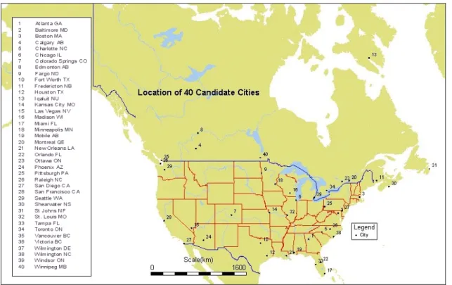
A candidate list of 40 cities was produced from which 5 cities were selected for the parametric study phase of Task 7. The list comprises the original list provided by the consortium members combined with

additional cities provided by the Task 4 team members. The locations of the cities are shown in Figure 1. Climate summaries for each of the candidate cities are provided in Appendix A.

City

Atlanta GA Fredericton NB Montreal QE St. John's NF

Baltimore MD Halifax NS New Orleans LA St. Louis MO

Boston MA Houston TX Orlando FL Tampa FL

Calgary AB Iqaluit NU Ottawa ON Toronto ON

Charlotte NC Kansas City MO Phoenix AZ Vancouver BC

Chicago IL Las Vegas NV Pittsburgh PA Victoria BC

Colorado Springs CO Madison WI Raleigh NC Wilmington DE

Dallas/Fort Worth TX Miami FL San Diego CA Wilmington NC

Edmonton AB Minneapolis MN San Francisco CA Windsor ON

Fargo ND Mobile AL Seattle WA Winnipeg MB

In summary, enough data were collected from official sources to give adequate coverage of the United States and Canada. The hourly data can be quickly converted into a format suitable for Advanced Hygrothermal Model or in other formats that can be used for statistical or other analyses. A detailed analysis for each of the 40 candidate cities was done to provide a basis for selecting of the five locations to be used in the parametric study.

Climate Indices

In order to select the five cities to be used as part of Task 7 a method of comparing climates was developed. The method combines measures of wetting and drying potentials into a moisture index that represents the potential for moisture loading. The moisture index was used to select the five cities from the candidate list of 40 cities.

Climate data, especially long-term data, is essential for characterizing the climate of particular location. Climate has a direct influence on human activity. Climate data however in its generic form is not

2

One of the most import generalizations in Climatology is that the variability of precipitation decreases with increasing precipitation. The mean for Chicago is 914 mm while the standard deviation is 152 mm.

(11)

meaningful in and of itself. In the range of rainfall from 25 mm to 2500 mm there is no particular value that is more important than any other. Similarly there is no particularly important temperature in the range from

-40 to 40 oC that is important except one - the value of 0 oC - which is the freezing point of water. It is

possible create meaningful indices from climate data that can be used for practical purposes. Examples of such indices are growing degree-days, heating degree-days, potential evapotranspiration (PET), and annual driving rain index (aDRI). Other building related indices are reviewed in the section on Climate Zoning

Figure 1. The map of North America shows the locations of the candidate cities.

Two indices were developed from the climate data. The indices were used to calculate a moisture index for the candidate cities. The moisture index was used to select the cities for the parametric study phase of Task 7 from the original candidate list. By using the climate indices it was also possible to select the Moisture Reference Years for the selected cities. Finally the indices were used as the basis for initial climate zoning of Canada and the United States.

The two indices developed to characterize the climates of the candidate cities are the wetting index (WI) and the drying index (DI). The wetting index describes the wetness of a particular climate, specifically the potential for a wall to get wet. The drying index describes the dryness of the climate or particular year, specifically the potential drying that could occur if a wall should get wet. The indices, wetting and drying, are independent. For example a particular year can be characterized as wet (lots of rain) while at the same time rank high on the drying scale (hot).

An important assumption used in the creation the two indices WI and DI is that the response of the wall is unknown. We purposely blinded ourselves to building types and wall characteristics in order to classify climates and years according to the available meteorological data.

The Wetting Index

(12)

effect of wind during rain, the annual driving rain index (aDRI). Either can be used as the basis for the wetting index. Cornick [1] compares how the candidate cities are ranked using both rainfall and aDRI. The annual driving rain index can be calculated from the basic climate parameters from Equation 1.

∑

= n 1 t U10 * Rh/1000 m2/sec-year (1)

where: U10 = hourly wind speed at 10 m

Rh = horizontal rainfall mm/m2-h

n is the number of hours in a year, i.e. either 8760 or 8784 hours.

For many locations however wind speed and direction data may not be available. If a measure of aDRI is required it can be roughly estimated as the product of the annual rainfall and average annual wind speed. Such estimates may however under-report the annual driving index by as much as 40% [3]. Driving rain maps have been constructed for many countries and the aDRI can be computed from them [4][5][6]. The other measure of water availability is the total average annual horizontal rainfall for a particular location. Rainfall and aDRI are strongly correlated [7] [8]. This is expected since the driving rain index is defined as a product of rainfall and wind speed, see Cornick [1]. Rainfall was the preferred parameter for defining the wetting index since that parameter is commonly available for most stations, even those that do not report hourly data. Unless otherwise noted the wetting index, WI, was defined as the mean annual total

horizontal rainfall3.

The Drying Index

The drying index (DI) was defined as the potential for a wall to dry once it has gotten wet. The

principle process for drying is evaporation4. For practical purposes there are two concepts of evaporation.

The first is Potential Evaporation (PET). This is essentially the amount of evaporation that would occur over the ocean. It represents the rate controlled entirely by atmospheric conditions and is the maximum possible. PET can be measured directly using evaporation pans. The other concept is Actual Evaporation (AET) which is the amount of the actual loss of water given the prevailing atmospheric and ground conditions. AET can be measured using a weighing lysimeter, in which a section of land surface is removed; a pan placed in the cavity and the land replaced with as little alteration to its initial structure as possible. Measurement of either PET or AET is difficult and not commonly available. Many evaporation models exist for predicting evaporation rates. They are not very helpful in that the input data required is not

readily available5.

3

Another definition for the wetting index, WI, will be given in the section on Moisture Reference Year. The wetting and drying indices can be defined arbitrarily to suit a particular application.

4

In the field of Climatology another measure is used, evapotranspiration. Evaporation occurs when there is a free water surface. Transpiration occurs when water is removed from the stomata of plant leaves. The combined process of evaporation and transpiration is called evapotranspiration. The forcing mechanisms are similar. They are: (1) energy availability, (2) the humidity gradient away from the surface, (3) the wind speed immediately above the surface, and (4) water availability. [9].

5

Estimates of evaporation can be made using the basic climate data. A formula for evaporation developed by Thornthwaite and Holzman is given in Trewartha [10] as an example.

E = 17.1* (e1 - e2) * (u2 - u1)/(t + 459.4)

where: E = evaporation in inches per day

e1, e2 = vapour pressure in inches at levels 1 and 2

u1, u2 = wind speed in mph at levels 1 and 2

(13)

A general approach is to assume that evaporation is proportional to the difference between saturation

vapour pressure, es, and the vapour pressure of ambient air, e [11]. The term es - e appears frequently in the

meteorological and hydrological literature. A variant of this general approach is the Π factor method [12]. The Π factor method lumps together various climate parameters into a single number and represents a type of drying out weather potential. The Π factor is defined in Equation 2.

∫ − = − − = b a out e sat out e sat a b period t t(v (T) v )dt v (T) v * ) t 1/(t Π (2)

where: Πperiod is the Π factor over the period ta to tb

vsat = the saturation humidity by volume at Te in kg/m3

vout = the outdoor humidity by volume in kg/m3

Te = is the equivalent surface temperature in oC

The overline mark signifies the average of the expression over the considered period. Te in this case is

similar to the Sol-air temperature defined in ASHRAE [13].

Te = Tout + 1/(αr + αc) * [Isol * αsol + αr* (Tr- Tout)] (3)

where: Tout is the outdoor air temperature in °C

Isol is the incident solar radiation on the wall surface W/m2

αsol is the surface solar absorption factor

αc_{and α}r

are the surface heat transfer coefficients in W/m2-K

r

T is the average sky temperature °C

A simple modified Π factor approach was adopted for defining the drying index, DI. The method does not

use the assumed characteristics of the wall needed to calculate Te. The drying index at time t is defined

simply as the difference between the humidity ratio (alternatively the mixing ratio) at saturation, wsat, and

the humidity ratio at ambient conditions.

∆w(t) = wsat(t) - w(t) kg water/kg air (4)

The humidity ratios can be calculated using Equation 5 and the equations given in Appendix B. Finally the drying index for a location can be calculated from Equation 6.

w = 0.622* (vp/(p - vp)) kg water/kg air (5)

where: w is the humidity ratio kg water/kg air

vp is the vapour pressure in kPa

p is the total mixture pressure in kPa

DI = (1/n)

∑

= n 1 i

∑

= k 1 h ∆w kg water/kg air-year (6)

where: DI is the drying index in kg water/kg air-year n is the number of years under consideration

k is the number of hours in a particular year, i.e. either 8760 or 8784 hours.

If hourly data are not available for a location the drying index, DI, can be calculated from the long-term annual average temperature and the average annual relative humidity. The correspondence between the DI

(14)

calculated using hourly weather data and the DI calculated using climate normals is good and is shown in Figure 2 [1]. Using the average annual temperature obtained from climate normals however can lead to a significant underestimation of the drying index. It is recommended that if the DI is to be calculated from

long-term averages that an equivalent average temperature, Teq, be used. The definition of the equivalent

temperature, Teq, is discussed in the section on Climate Zoning.

Predicted Drying Index versus Calculated

R2_{= 0.9743} 0 20 40 60 80 100 120 140 0 20 40 60 80 100 120

Calculated (Hourly) Drying Index kg water/kg air

Predicted (Climate Normal) Drying Index kg water/kg air

City Linear Fit

Figure 2. The figure shows the mean drying index for a city calculated from hourly weather data plotted against the drying index calculated using long-term climate normals.

It should be noted that the method for calculating drying potential outlined above is a variation of the concept of Potential Evaporation (PET).

Application

The drying and wetting indices can be calculated for each individual year for a particular location or for a long-term mean value, representing a climate. Figure 3 shows a plot of drying index versus wetting index for five cities calculated using hourly values. Each point represents a specific year in the hourly weather record for each city. The wetting index in this case is defined as the total rainfall for the year and drying index is calculated for each year as described previously. The ellipses bound the years for each city and show the range and variation of WI and DI for each city.

The characteristics of a particular climate can been be inferred from the general position of the ovals on the plot. Cities in the upper left hand corner, Phoenix for example, have a high drying index and a low wetting index and can be characterized as not having a high potential for moisture loading. Cities occupying the lower right hand corner of the plot however have low drying indices and high wetting indices and can be assumed to have a higher potential for moisture loading. The plot also suggests that the potential moisture loading would increase with increasing wetting index. Intuitively this seems to be borne out by the

(15)

severity the order would be Winnipeg, Ottawa, Seattle and Wilmington. This kind of plot, while useful in examining the range and variability of a climate, is not so useful in comparing climates quantitatively with one another.

Drying Index versus Wetting Index (Precipitation)

0 20 40 60 80 100 120 140 160 180 0 200 400 600 800 1000 1200 1400 1600 1800 Precipitation (mm) D rying Inde x (kg w ate r/kg a ir) Phoenix AZ Wilmington NC Seattle WA Ottawa ON Winnipeg MB

Figure 3. The plot shows DI and WI for individual years for five selected cities. The plot shows the range and variability of both indices as well as the relative characterization of the general climates found in those cities.

If the mean values for DI and WI are plotted instead of the individual years the ellipses in Figure 3 are essentially collapsed. The resulting scatter plot is shown in Figure 4. The plot is similar to the previous plot except that all 40 candidate cities are included. The problem of characterizing climate however remains. Only qualitative comparisons are possible using this approach. Qualitative comparisons are also hard to make without some idea of what weight to give the drying index (kg water/kg air-year) relative to the wetting index (mm/year). For Task 4 the drying and wetting were given equal weights.

A Ranking Method: The Moisture Index

A ranking method was developed so that quantitative comparisons between climates could be

made. The wetting index and drying index were combined into a single number, a moisture index, MI6. The

hypothesis is that the higher the value of the moisture indices the greater the potential for moisture loading. The first step in ranking cities is to normalize both WI and DI with respect to minimum and maximum values in the sample set. This normalization scheme depends on which cities are included in the sample set.

6

"A moisture index is a device which allows better comparison of natural landscapes than can be gained from the distribution of simple rainfall amounts. Such an index is then a more refined expression of the moisture factor in climate than straight rainfall, an advantage claimed for the simple indices proposed by

(16)

If the range of WI and DI is changed significantly a different ranking will result. This will be discussed further in the section on Climate Zoning. The relative comparison scheme is a consequence of the decision not to consider the wall response as part of the climate analysis. The forty candidate cities cover for the most part the range of practical values for WI and DI.

Inormalized = (I - Imin)/(Imax - Imin) (7)

Drying Index versus Wetting Index (Precipitation)

0 20 40 60 80 100 120 140 0 200 400 600 800 1000 1200 1400 1600 1800

Wetting Index (Precipitation mm)

Dr y ing Index ( k g water /k g ai r) City

cold dry cold wet

hot wet hot dry

Figure 4. The scatter plot shows the mean DI and WI for the 40 candidate cities. The plot shows the relative characterization of the general climates for the candidate cities, the upper left quadrant being hot dry climates, the upper right being hot humid climates, the lower left being cold dry climates and the lower right being cold wet climates..

For the wetting index severity increases from zero to one, while severity for the drying index decreases from zero to one. Figure 5 shows a plot of the normalized indices. The plot is essentially the same as Figure

4 except that on the vertical axis 1 - DInormalized is plotted. The potential for moisture loading increases with

increasing values of x and y. A point near the origin, (0, 0), consequently would have the lowest potential for moisture loading while the point furthest from the origin, (1,1) would have the highest. The MI for each city is calculated as the distance from the origin. Again wetting and drying were assumed to be of equal importance and thus they were given equal weight in the determination of the moisture index. If the wall response is to be considered a weighting factor could be introduced.

2 normalized 2 normalized (1 DI ) WI MI= + − (8)

(17)

Drying Index versus Wetting Index 0 0.1 0.2 0.3 0.4 0.5 0.6 0.7 0.8 0.9 1 0 0.1 0.2 0.3 0.4 0.5 0.6 0.7 0.8 0.9 1

normalized Wetting Index (Precipitation)

1 nor m a liz ed Dr y ing Index MI = (x2 + y2)0.5 Phx Wil Win Ott Sea

Figure 5. A plot of 1 - normalized Drying Index versus normalized Wetting Index (rainfall) for the candidate cities. The moisture index is calculated as the distance from the origin.

Using this method it is possible to assign each city in the candidate list a moisture index. The table below shows the moisture index for the five cities mentioned above. Cornick [1] provides the indices for all the candidate cities using both rainfall and aDRI as the wetting index.

WI = rainfall WI = aDRI City MI City MI Wilmington NC 1.133828 Wilmington NC 0.91934 Seattle WA 0.98935 Seattle WA 0.909885 Ottawa ON 0.927398 Ottawa ON 0.872317 Winnipeg MB 0.86177 Winnipeg MB 0.847528 Phoenix AZ 0.125075 Phoenix AZ 0.081777

This method of calculating the moisture index is general. Any definition of wetting and drying can be assumed for the wetting and drying indices. The choice is dependent on the application as will be seen in the following section on the Moisture Reference Year.

The Five Cities and Alternates

From the list of 40 candidate cities five were chosen for the parametric study phase of Task 7. The five cities are: (1) Wilmington NC, (2) Seattle WA, (3) Ottawa ON, (4) Winnipeg MB, and (5) Phoenix AZ. Three other cities were selected as alternates. They are: (1) Vancouver BC, (2) Shearwater NS, and (3) San Diego CA. Climate summaries for the selected and alternate cities are given in Appendix C. The five cities chosen from the candidate list span the range of rankings. Of the five selected cities two fall into the top one third of the rankings (Wilmington and Seattle). Two others were selected from the middle third of the ranked list (Winnipeg and Ottawa). The final city was selected from the bottom third (Phoenix).

(18)

City (Selected) Moisture Index Köppena Russoa

Wilmington NC Top third Subtropical Humid Hot Wet

Seattle WA Top third Temperate Oceanic Cool Summer Mild Wet

Ottawa ON Middle third Temperate Continental Cool Summer Cold Wet

Winnipeg MB Middle third Temperate Continental Cool Summer Cold Dry

Phoenix AZ Bottom third Arid Hot Hot Dry

City (Alternate)

Vancouver BC Top third Temperate Oceanic Cool Summer Mild Wet

Shearwater NS Top third Temperate Continental Cool Summer Cold Wet

San Diego CA Bottom third Subtropical Dry Summer Hot Dry

a - see Appendix D for a description of climate classification schemes

Moisture Reference Years

Recall that the main objective of Task 4 - Environmental Conditions was to characterize climate to be used as parameter for the Task 7 parametric study. Having selected five cities from the candidate list of 40 the next step was to determine what years from the data record for the five selected cities to use as input for the Advanced Hygrothermal Model. This section outlines the development of a method for selecting moisture reference year(s).

Defining The Moisture Reference Year

The problem of defining a Moisture Reference Year (MRY) or Moisture Design Year for hygrothermal analysis is ongoing. The International Energy Agency (IEA), in Annex 24 (on Heat-Air and Moisture Transport) Task 2 Environmental Conditions, has made recommendations on how to determine a moisture design year [15]. Some of the methods require the use of specific building and wall

characteristics. Since the approach taken in Task 4 was that the climate data would be treated independently of the wall response many of the IEA recommendations do not serve the purposes of this project. A

universal method for selected a moisture reference year is not currently available. Karagiozis [16] points to other researchers contributing in this area including: Geving[17], Kuenzel [18], and Hagentoft [19]. The problem still remains as to what to select as input for the parametric study phase of Task 7. One approach is to use the entire hourly weather record, 30 to 40 years, as input. This approach is currently not practical. Another approach is to define a reference year similar to the energy reference years that have been developed for energy calculations. Energy reference years are statistical years in that the values for each hour are synthesized from statistical analysis. Examples of statistical years include, typical reference year (TRY), typical meteorological year (TMY), and weather years for energy calculations (WYEC2 and CWEC). Again this is ongoing problem, currently being addressed for example by ASHRAE Technical Committee 4.2 [20].

Using the Climate Indices for Selecting Years

The approach taken in MEWS to selecting weather data for input to the AHM is to construct an input file spanning three years using actual weather data. Using the wetting and drying indices it is possible to classify individual years as wet, dry, or average. From the weather record for a particular city the drying and wetting indices are calculated for each year. A moisture index for each year is calculating using the same technique used in climate classification. The hypothesis here is the same as the climate classification hypothesis; the higher the moisture index the greater the potential for moisture loading. Wet and dry years can be defined as those years that deviate more than one standard deviation from the mean. Average years can be defined as being within one standard deviation. For MEWS the wet year for a city is defined as the year with highest moisture index, the dry year as the year with lowest moisture index, and the average year as the year closest to the mean moisture index. Figure 6 shows the three years selected as wet, dry and

average for Wilmington NC. The chart shows the deviation of the drying and wetting indices from the

(19)

Figure 6. The plot shows the deviations of individual years from the means of the climate indices for Wilmington NC. The dark line shows the deviation from the mean for the wetting index. The light line shows the deviation from the mean for the drying index. Years selected as wet, dry and average are highlighted. The selection was based on the moisture index.. The dry year can be seen to have a higher than normal drying index and a lower than normal wetting index. The combination produces the lowest moisture index.

It is now possible to select the moisture reference years to be used for the parametric study phase of Task 7. Years can be classified as wet, dry, or average. The required three-year span is then synthesized by

concatenating three individual years together to form the desired three-year span. The method provides for great flexibility in creating patterns for the three year span.

Charts similar to the one shown in Figure 6 were developed by Cornick [1] for Miami and Vancouver. For those cities it was noted that there was only one occurrence of two consecutive years with rainfall

exceeding one standard deviation (i.e. 5% probability of occurrence) over 35 years for both cities. There were no observed intervals with three consecutive years of rainfall above one σ. One possible pattern for the three year span could have the first two years classified as wet with the following year being classified as average. Many other plausible patterns, up to 27, can be constructed for the three-year span required for the parametric study phase of Task 7.

Predominate Direction

One further input was needed for Task 7 – the directional component of rainfall. Up to this point the definitions of the drying index and wetting index have been defined without considering directional components. The wetting index was defined as the total average annual rainfall on the horizontal. The definition of the drying index is omni-directional. The scope of the parametric study phase was limited to analyzing one wall orientation. This required a redefinition of the wetting index, WI.

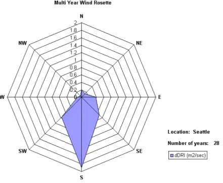
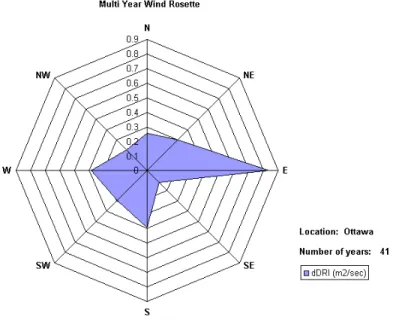
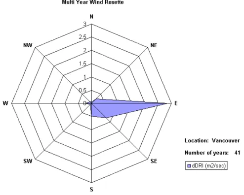
Figure 7 shows 4 years selected from the Wilmington NC weather record. The directional driving rain indices (dDRI) for two wettest years, the average year, and the dry year are shown. In selecting these years the WI was equal to the annual rainfall on the horizontal. Suppose that the orientation of a given wall is South. The Advanced Hygrothermal Model will impose a rain load on the wall in proportion to the wind

(20)

year, 1968 a North or North East orientation would be preferable. Clearly if only one wall orientation is to be considered a directional component must be introduced to the wetting index. The nature of the drying processes considered here does not require the introduction of a directional component into the drying index.

Directional Driving Rain Rosette (m2/sec)

0 0.5 1 1.5 2 2.5 3 N NE E SE S SW W NW 1989 wet 1966 wet 1968 dry 1979 average 1989 1966 1968 1979

Figure 7. This rosette shows the directional driving rain indices for four years selected from the weather record for Wilmington NC. The years were classified as wet, average, or dry using the ranking method described in the previous section.

The first step in introducing a directional component was to determine the predominant direction of rainfall as it relates to wind speed and direction. Long-term average directional driving indices for each the selected cities are given in Appendix C. Some locations display an obvious predominant direction while for others the predominant direction is not immediately apparent.

To determine the predominant direction of rainfall the rain load on the wall was calculated for the four cardinal orientations for each city. The method used to calculate the rain load was recommended by

Straube7[21]. Straube's and other related methods will be discussed in the following section.

The total amount of rain impinging on the wall was calculated for all the years available for a city. The direction with highest amount of total rain impinging on the wall was selected as the predominant direction for rainfall. In cases where there was little difference between the total amounts, such as Wilmington NC, the predominant direction was selected, conservatively, to be the one least conducive to drying. For

Wilmington NC the direction selected was North; the orientation with the least direct solar radiation8.

7

In fact 5 methods including Straube's were used for comparison. 8

Although the drying index is directional independent, comprising temperature and relative humidity, the AHM does consider the effect of orientation by including solar radiation and wind. Thus a north facing

(21)

Location: Wilmington NC Years = 22 Orientation

Method North East South West

Total Straube mm/m2 9369 8472 9251 2784

Total Lacy mm/m2 9871 8987 9862 2821

Total LIF mm/m2 6846 6260 6911 1913

Total UK method mm/m2 5422 5000 5568 1438

Total AHM mm/m2 3525 3220 3547 988

Total dDRI m2/sec 54.33 50 55.68 14.37

The predominant direction for Wilmington NC based on Straube's method is North

The reference years for the selected cities were calculated using the same classification scheme outlined above. The years selected as wet, dry, and average for the five selected cities and three alternates are given in appendix E. The major difference between classification schemes for climates and reference years is the redefinition of the wetting index, WI. The wetting index for selecting reference years is defined as the annual rain load on wall in the predominant direction of rainfall. The redefined wetting index derived from Straube's [ 21] method is given in Equation 9. A detailed description of the method is given Appendix F.

WI = RAF * DRF(rh) * cos (θ) * V(h) * rh (9)

where: WI is the wetting index

RAF is the rain admittance factor

rh is the horizontal rainfall intensity mm/m2-h

V(h) is the wind speed at the height of interest m/sec θ is the angle of the wind to the wall normal

Review of Micro-Climate Models

The final step in providing weather data to the simulation phase of Task 7 - Hygrothermal

Analysis was to establish the exterior boundary conditions at the surface of the wall; in effect to bring the

weather to the wall. A study was undertaken, as part of Task 4, to collect in-situ measurements of the rain impinging on building facades and to compare the measured results with various prediction models. Details of this study are provided by Straube [21]. Five methods for calculating the rain load impinging on the surface were reviewed and the measured data show a good correspondence with the predicted results. The five methods are briefly described in Appendix F. Straube's method, slightly modified, was adopted as the method for calculating the wind driven rain loads.

Input to Task 6, System Performance, was also provided here. The Dynamic Wall Test Facility protocol for Task 6 was intended to represent wind-driven rain conditions for low buildings anywhere in North

America. The two spray intensity rates and the maximum static pressure level for the rain penetration tests were derived from the climate data and the literature and modeling results using the CFD-LIF approach outlined in Appendix F. Dalgliesh [22] describes the procedure used in determining both the spray rates and

maximum static pressure level. The recommendation for the two spray rates are 100 L/m2-h (1.7 L/min-m2

)

and 200 L/m2-h (3.4 L/min-m2

). A maximum static pressure of 700 Pa +/- 300 Pa at 0.50 Hz is recommended.

Part II - Climate Zoning

(22)

Climate Classification Schemes

There are several different schemes for classifying the world's climate, most them possessing genuine merit. Almost all of the schemes of climate classification have subdivisions and boundaries partly based upon temperature and rainfall parameters which are not meaningful in themselves, but have

significance in terms of some nonclimatic feature such as vegetation, human comfort, mold growth, wood rot, or the like. If one disregards nonclimatic phenomena, it is difficult to provide meaningful temperature-rainfall limits of climatic types. The majority of classification schemes, therefore, are of an "applied" character. Some classification schemes are outlined in Appendix D.

One basis for grouping climate schemes is to divide them into genetic and empirical types. In genetic classifications an attempt is made to group climates into the causative factors (e.g. air masses, wind zones) that may be responsible for them. In empirical classifications, origin is discarded as an organizing principle, and observation and experience provide the essential elements for climatic differentiation. The Köppen classification scheme (reviewed in Appendix D) represents a combined genetic-empirical classification while Russo's and Scheffer's classifications are empirical in nature. The classification developed here is also an empirical classification.

Climate Zoning Using the Climate Indices - Proposed Method

The climate indices developed for ranking the candidate cities were used as the basis for

developing a climate classification. The wetting index, WI, was defined as the total average annual rainfall. The drying index, DI, was defined as a measure of potential evaporation using a modified Π-factor approach, outlined above. The ranking of cities was done using the normalized ranking method described

previously. The moisture index, or ranking, ranges from 0 to 1.414 ( 2 ). Again, the hypothesis is that the

higher the moisture index the greater the potential for moisture loading, with an index value of zero

representing a climate with little or no potential. An index value of 2 represents a climate with a

maximum potential for moisture loading. Grouping Climates

Having established a procedure for ranking climates the next step was to divide the range of the moisture index creating groupings of climates, i.e. classifications. The range of the moisture index can be, for example, split into three divisions. Since the moisture index is defined as the distance that a climate lies from the origin on a normalized plot (see Figure 5) the boundary values for the groupings can be expressed as radii.

Suppose a particular location has a normalized wetting index, WInormalized, of one, indicating maximum

wetting potential, and a normalized drying index, DInormalized, of one, indicating maximum drying potential.

This climate corresponds to the point (1, 0) on the plot shown in Figure 8. Note that 1 - DInormalized rather

the Dnormalized is plotted on the y-axis. This ranking corresponds to a radius, r, equal to one. Similarly a

climate having WI = 0, minimum wetting, and DI = 0, minimum drying, corresponds to the point (0, 1) in Figure 8. This climate also lies on the arc r = 1.

Although both these climates might be different in terms of wetting (rainfall) and drying (temperature and relative humidity) characteristics the hypothesis is that they are in similar with respect to the potential for moisture loading. Using an analogy to Mohr's circle the points along a radius are hypothesized to have an equal potential for moisture loading; an isopotential.

(23)

Figure 8. The plot shows a classification scheme based on a hypothesis of isopotentials. Each radius defines a locus of points having an equal potential for moisture related problems.

A simple classification can be constructed by splitting the range of the moisture index into three divisions along three isopotentials. The climates are then grouped accordingly. The map shown in Figure 9 represents such a classification. The map shows he grouping of the 40 candidate cities. The assumption for selecting the boundary for the high potential is the points (1, 0) and (0, 1) in Figure 8 are critical points. The point (1,0) representing maximum wetting and maximum drying was deemed critical because of the availability of large amounts of water. Similarly the point (0, 1) representing minimum wetting and minimum drying was deemed critical because of the poor drying potential.

Division (radius in Figure 8) Classification w.r.t. Moisture Loading Colour

MI greater or equal to 1.0 High Red

MI greater or equal to 0.9 but less than 1.0 Moderate Yellow

MI less than 0.90 Low Green

A Provisional Map

A more detailed map of the USA and Canada was constructed using 383 stations reporting hourly data. Instead of using hourly values to compute the rankings for each station long-term data obtained from climate normals were used. The current climate normals span the years 1961 to 1990. The wetting index, WI, was defined, as before, as the annual average rainfall on the horizontal. The drying index was

computed using the method described above except that the average annual temperature and average annual relative humidity were used instead of hourly values. Why use annual averages instead of hourly values in calculating the moisture indices for the provisional map? There were two reasons: 1) to save time and, 2) to develop and test a method appropriate for codes and standards. In order to use climate normal data a slight refinement of the method for the calculating the drying index however was necessary.

For the purposes of Task 4 all values for the drying index were calculated from the sum of the hourly values; the hourly method. This method is considered to be exact. In making the provisional map however long-term climate normals were used. When climate normals are used to calculate the drying index, the

annual method, considerable underestimation of the potential evaporation can be introduced. To correct for

this a temperature correction is applied to the long-term temperatures obtained from the climate normals.

This correction yields an equivalent temperature, Teq, which produces approximately the same drying index

(24)

City Rain DI MI City Rain DI MI

Mobile AB 1639.5 39.14 1.22 Pittsburgh PA 931.1 30.19 0.95

New Orleans LA 1601.4 36.44 1.21 Tampa FL 1113.7 44.14 0.95

St Johns NF 1193.8 10.20 1.17 Madison WI 803.9 24.67 0.95

Shearwater NS 1178.1 13.11 1.15 Windsor ON 788.4 24.27 0.94

Wilmington NC 1406.4 33.48 1.13 Montreal QE 737.4 22.07 0.94

Vancouver BC 1058.2 16.10 1.09 Ottawa ON 701.8 22.96 0.93

Miami FL 1464.0 50.13 1.08 Kansas City MO 967.6 36.96 0.93

Atlanta GA 1306.0 39.02 1.06 St. Louis MO 959.6 37.19 0.92

Orlando FL 1274.1 41.69 1.03 Toronto ON 625.6 21.58 0.92

Boston MA 1057.6 29.00 1.01 Minneapolis MN 729.2 28.24 0.90

Houston TX 1211.4 41.14 1.01 Edmonton AB 359.9 19.73 0.88

Victoria BC 813.0 17.03 1.00 Winnipeg MB 390.5 22.24 0.86

Fredericton NB 847.8 19.84 0.99 San Francisco CA 506.6 25.58 0.86

Seattle WA 927.4 24.38 0.99 Fargo ND 500.9 26.11 0.85

Wilmington DE 1037.6 31.85 0.98 Calgary AB 293.4 26.71 0.81

Raleigh NC 1046.0 34.44 0.97 Fort Worth TX 857.3 53.57 0.79

Iqaluit NU 257.8 6.12 0.97 San Diego CA 266.6 36.41 0.74

Charlotte NC 1094.6 39.48 0.96 Colorado Springs CO 424.5 45.33 0.70

Baltimore MD 1026.1 34.87 0.96 Phoenix AZ 205.1 129.47 0.13

Chicago IL 914.3 29.01 0.96 Las Vegas NV 108.2 117.78 0.11

MI is based on hourly values; Rainfall is in mm; DI is kg water/kg air. To calculate MI use the procedure outlined above. Normalize the wetting index using Mobile AB. Normalize the drying index using Phoenix AZ.

(25)

One further change was introduced in producing the provisional climate map. The maximum rainfall used

to normalize the wetting index was set at 2000 mm.9 Strictly speaking the wetting index is no longer

normalized since several stations have normalized indices greater than one. Setting the maximum rainfall at 2000 mm was done because stations with large annual rainfall averages push the rankings of the majority of stations into ranges where little or no potential moisture loading is hypothesized to exist. North America then becomes divided into two zones, the north west coast (excluding relatively sheltered locations such as Seattle and Vancouver) and the rest of the continent. This seems to be at odds with practical experience. Indeed the stations that report over 2000 mm of rainfall are extreme, especially those on the littoral of North American northwest coast (see Figure 10), when compared to rest of the stations considered for the provisional map. Limiting the maximum rainfall in the normalization procedure produces a more useful map.

WBAN Station Name State Rainfall (mm) T (C) RH %

25339 YAKUTAT AK 3349.0 3.9 80.5 21504 HILO HI 3281.4 23.3 74 94234 TOFINO A BC 3235.8 9.0 85 94240 QUILLAYUTE WA 2638.3 9.4 83 41415 GUAM PI 2617.2 26.0 81 25308 ANNETTE AK 2501.1 7.7 76.5 25353 PRINCE RUPERT A BC 2409.1 6.9 82

Note the low temperatures and high RH and Rainfall on the Northwest coast of NA

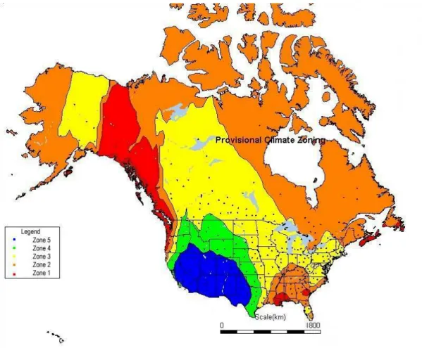
Five divisions were used to create the provisional map. The classifications are: Zone 1, Zone 2, Zone 3,

Zone 4, and, Zone 5. A classification of extreme is given to all stations having a ranking of greater than √2;

all the stations discussed above are classed as extreme. In creating the provisional map all extreme stations were included in the Zone 1 category. The map is shown in Figure 11 and shows good agreement between it and other construction related climate classification schemes (see Appendix D). A few comments on the provisional contour map are worth mentioning. The first is that in generating a contour map a certain amount of information is lost. For example, the reporting station for Flagstaff AZ is classified as having a

Zone 4 potential. However, during the process of generating the contour map the area surrounding Flagstaff

is included in Zone 5. The data used to generate the contour map is two steps removed from the original data points. Appendix H provides a primer on contour map generation.

Second, the network of reporting stations used to generate the map is sparse in the northern regions of the continent. The contour map could be improved, especially in the extreme northwest section, with inclusion of more data points.

Summary information for all 383 reporting stations is given in Appendix G. The opportunity for future work presents itself here. Specifically, the climate classification (i.e. the Moisture Index) needs to be correlated to quantitative amounts of moisture related damage such as mould growth, wood decay, or metal corrosion. The measures of damage could be observed in the field, obtained experimentally, or derived from computer models.

Division Classification w.r.t. Moisture Loading Colour

MI greater or equal to 1.0 Zone 1 Red

MI greater or equal to 0.9 but less than 1.0 Zone 2 Orange

MI greater or equal to 0.8 but less than 0.9 Zone 3 Yellow

MI greater or equal to 0.7 but less than .0.8 Zone 4 Green

MI less than 0.70 Zone 5 Blue

(26)

Figure 9. The map of North America shows the classification of the 40 candidate cities with respect to their potential for moisture loading.

Figure 10. The map shows the location of all the continental stations considered that report more than 2000 mm of rainfall. There are all on the North American northwest coast littoral. These stations are considered extreme with respect to moisture loading.

(27)

Figure 11. The contour map shows the isopotential lines for moisture loading. The classification is based on five divisions of the range of values of the moisture index. 383 hourly reporting stations were used to generate the map. The reporting stations are shown as points on the map.

Conclusions

For the purposes of characterizing the moisture loading in building envelopes climate can be described using two indices, a wetting index which is a function of rainfall, and a drying index which is function of potential evaporation. These two indices are independent. Climates can be classified by defining a moisture index that combines the wetting and drying indices. The moisture index can then be used to rank weather stations according to their potential resulting in a climate classification scheme. Thus climates with dissimilar wetting and drying characteristics can be compared directly using the moisture index. The moisture index can be considered as an indicator of potential moisture loading in building envelopes. Isopotential lines can be created by joining stations with similar moisture indices. In this way maps showing the potential for moisture loading can be drawn. Selecting the values of the isopotentials completes the classification scheme. This approach is consistent with previous approaches that have been developed to assess such quantities as crop yield, wood rot and mould growth, and corrosion of metals. The same methodology developed for classifying climates can be used to compare individual years from the climate record for a particular location. Years can be classified as either wetter than average or drier than average, or average based on the moisture index. Moisture reference years suitable for heat, air, and moisture transport models can be selected from weather records using this methodology.

(28)

Several issues remain to be resolved in relation to the Task 4 work. The three most important are:

1. Relative comparisons - The ranking of climates and reference moisture years is based on a relative ranking rather than objective criteria. This disadvantage was overcome by selecting a set of climates that would adequately span a range of possible values for Canada and the United States. This is less of an issue for selecting moisture reference years since the number of years available is likely to cover the expected range for a weather station. The lack of objective criteria and hence the relative ranking scheme is a direct consequence of not specifying what constitutes a moisture problem. Consequently the analysis of climate did not include the wall response to environmental conditions.

2. Equal weighting of WI and DI - The assumption is that the wetting and drying indices have equal weights when combined. This may or may not be correct. Again this is due to the initial decision not to consider the wall response. Better estimates for the weighting factor might be forthcoming after analysis of the Task 7- Parametric Simulation and Task 5 - Damage Functions results. 3. Selecting values of the isopotentials - The setting of the values of the isopotentials for purposes of

climate zoning was arbitrary and based on the judgment of the authors. Once the results of Task 7 and Task 5 have been analysed better estimates of the values for the isopotentials might be established. To obtain meaningful values however decisions must be made as to what factors relate to long-term wall performance; for example how do decay, corrosion, staining, finish deterioration, production of molds and spores, loss of structural capacity, degradation of thermal resistance, water damage to interior finishes and furnishings, and dimensional changes effect the appearance or functioning of the wall system?

There are criticisms of the Task 4 approach. The two main criticisms are:

1. No recognition of wet or dry spells.- The work presented here is based on an annual analysis. Looking at climate from the perspective of wetting and drying spells was not presented here. This can be done and in fact is being developed in order to compare with the approach taken here. This approach will not however resolve the issue of relative rankings.

2. Seasonal effects not considered. - This is similar to the criticism of not recognizing wet spells. Wetting is strongly dependent on the rain regime of the climate under consideration, the winter rain regime of subtropical dry summer (Cs) climates for example. Should credit by given to the drying potential that occurs in the summer when little or no rain falls? Analysis of the Task 7 and Task 5 results should help in answering such questions. Further refinements of the wetting and drying indices are possible.

Determining the potential for moisture loading for various climates, and individual years can be done using a simple method that uses readily available climate data, specifically climate normal data. The

methodology is general and flexible and involves defining a wetting index, based on the availability of water, and a drying index, based on potential evaporation. These indices are combined to form a moisture index. By redefining the wetting index and or drying index as well as changing the relative weighting between the two, further refinement can made in the final moisture index.

Summary

Hourly data for approximately 400 Canadian and US locations were collected. The number of years available for each location spans 30 or more years. A list of 40 candidate cities was created. Weather data for the 40 cities, 27 American and 13 Canadian, were analyzed and converted into the appropriate format for the Advanced Hygrothermal Model (AHM).

Two independent climate indices, the wetting index, WI, and the drying index, DI, were defined to characterize climates. The wetting index was defined as the average total annual rainfall although the annual driving rain index, aDRI, can be used without significantly changing the final results. The drying index was defined as average annual potential evaporation for a given location. The potential evaporation was defined as the "head room" in a parcel air available for moisture take up. This "head room" is