Mining for Availability Models in Large-Scale Distributed Systems:A Case Study of SETI@home

HAL Id: inria-00375624

https://hal.inria.fr/inria-00375624

Submitted on 15 Apr 2009

HAL is a multi-disciplinary open access

archive for the deposit and dissemination of

sci-entific research documents, whether they are

pub-lished or not. The documents may come from

teaching and research institutions in France or

abroad, or from public or private research centers.

L’archive ouverte pluridisciplinaire HAL, est

destinée au dépôt et à la diffusion de documents

scientifiques de niveau recherche, publiés ou non,

émanant des établissements d’enseignement et de

recherche français ou étrangers, des laboratoires

publics ou privés.

Mining for Availability Models in Large-Scale

Distributed Systems:A Case Study of SETI@home

Bahman Javadi, Derrick Kondo, Jean-Marc Vincent, David P. Anderson

To cite this version:

Bahman Javadi, Derrick Kondo, Jean-Marc Vincent, David P. Anderson. Mining for Availability

Models in Large-Scale Distributed Systems:A Case Study of SETI@home. [Research Report] 2009.

�inria-00375624�

Mining for Availability Models in Large-Scale Distributed Systems:

A Case Study of SETI@home

Bahman Javadi

1

, Derrick Kondo

1

, Jean-Marc Vincent

2

, David P. Anderson

3

1

INRIA, France,

2

University of Joseph Fourier, France,

3

UC Berkeley, USA

Abstract

In the age of cloud, Grid, P2P, and volunteer distributed

computing, large-scale systems with tens of thousands of

unreliable hosts are increasingly common. Invariably, these

systems are composed of heterogeneous hosts whose

indi-vidual availability often exhibit different statistical

prop-erties (for example stationary versus non-stationary

be-haviour) and fit different models (for example Exponential,

Weibull, or Pareto probability distributions). In this paper,

we describe an effective method for discovering subsets of

hosts whose availability have similar statistical properties

and can be modelled with similar probability distributions.

We apply this method with about 230,000 host availability

traces obtained from a real large-scale Internet-distributed

system, namely SETI@home. We find that about 34% of

hosts exhibit availability that is a truly random process, and

that these hosts can often be modelled accurately with a

few distinct distributions from different families. We believe

that this characterization is fundamental in the design of

stochastic scheduling algorithms across large-scale systems

where host availability is uncertain.

1

Introduction

With rapid advances in networking technology and

dra-matic decreases in the cost of commodity computing

com-ponents, large-scale distributed computing platforms with

tens or hundreds of thousands of unreliable and

heteroge-neous

hosts are common. The uncertainty of host

avail-ability in P2P, cloud, or Grid systems can be due to the

host usage patterns of users, or faulty hardware or software.

Clearly, the dynamics of usage, and hardware and software

stacks are often heterogeneous, spanning a wide spectrum

of patterns and configurations. At same time, within this

spectrum, subsets of hosts with homogeneous properties

can exist.

So one could also expect that the statistical properties

(stationary versus non-stationary behavior for example) and

models of host availability (Exponential, Weibull, or Pareto

for example) to be heterogeneous in a similar way. That is,

host subsets with common statistical properties and

avail-ability models can exist, but differ greatly in comparison to

other subsets.

The goal of our work is to be able to discover host

sub-sets with similar statistical properties and availability

mod-els within a large-scale distributed system. In particular, the

main contributions are as follows:

• Methodology. Our approach is to use tests for

random-ness to identify hosts whose availability is independent

and identically distributed (iid). For these hosts, we

use clustering methods with distance metrics that

com-pare probability distributions to identify host subsets

with similar availability models. We then apply

pa-rameter estimation for each host subset to identify the

model parameters.

• Modelling. We apply this method on one of the largest

Internet-distributed systems in the world, namely

SETI@home. We take availability traces from about

230,000 hosts in SETI@home, and identify host

sub-sets with matching statistical properties and

availabil-ity models. We find that a significant fraction (34%)

of hosts exhibit iid availability, and a few distributions

from several distinct families (in particular Gamma,

Weibull, and Log-Normal) can accurately model the

availability of host subsets.

These results are essential for the design of stochastic

scheduling algorithms for large-scale systems where

avail-ability is uncertain.

In the next section, we describe the application context

that is used to guide our modelling. In Section 3, we define

availability and describe how our availability measurements

were gathered. In Section 4, we contrast this measurement

method and our modelling approach to related work. In

Sec-tion 6, we determine which hosts exhibit random,

indepen-dent, and stationary availability. In Section 7, we describe

the clustering of hosts by their availability distribution. In

Section 8, we describe the implications of our results for

scheduling, and in the last section, we summarize our

find-ings.

2

Application Context

We describe here the context of our application, which

is used to guide what we model. Our modelling is

con-ducted in the context of volunteer distributed computing,

which uses the free resources of Internet-distributed hosts

for large-scale computation and storage.

Currently this

platform is limited to embarrassingly parallel applications

where the main performance metric is throughput. One of

the main research goals in this area is to broaden the types

of applications that can effectively leverage this platform.

We focus on the problem of scheduling applications

needing fast response time (instead of high throughput).

This class of applications includes those with batches of

compute-intensive tasks that must be returned as soon as

possible, and also those whose tasks are structured as a

di-rected acyclic graph (DAG).

For these applications, the temporal structure of

avail-ability and resource selection according to this structure is

critical for their performance. The temporal structure of

availability is important because many applications cannot

easily or frequently checkpoint due to complexities of its

state or checkpointing overheads.

Resource selection is important because in our

experi-ence and discussions with application scientists the

max-imum number of tasks in a batch for fast turnaround is

needed is much lower than the number active and available

hosts at a given time point (hundreds of thousands). This

same is true for the maximum number of tasks available in

a DAG application during its execution.

A

1

Time

CPU

on host i

A

2

A

n

Figure 1. CPU availability intervals on one

host

Thus our modelling focuses on the interval lengths of

continuous periods of CPU availability for individual hosts.

We term this continuous interval to be an availability

inter-val (see Figure 1). The lengths of the availability interinter-vals

of a particular host over time is the process that we model.

Using these models, a scheduler should then be able to

compute accurately the probability of successful task

exe-cution in some time frame, given a task’s exeexe-cution time.

Moreover, the scheduler could compute the probability of

success when task replication is used.

3

Measurement Method for CPU Availability

BOINC [5, 2] is a middleware for volunteer distributed

computing. It is the underlying software infrastructure for

projects such as SETI@home, and runs across over 1

mil-lion hosts over the Internet.

We instrumented the BOINC client to collect CPU

avail-ability traces from about 230,000 hosts over the Internet

be-tween April 1, 2007 to January 1, 2009. We define CPU

availability to be a binary value indicating whether the CPU

was free or not. The traces record the time when CPU starts

to be free and stops.

Our traces were collected using the BOINC server for

SETI@home. The traces are not application dependent nor

specific to SETI@home because they are recorded at the

level of the BOINC client (versus the application it

exe-cutes). In total, our traces capture about 57,800 years of

CPU time and 102,416,434 continuous intervals of CPU

availability.

Artifacts due to a measurement method or middleware

itself are almost inevitable. In our case, artifacts resulted

from a benchmark run periodically every five days by the

BOINC client.

As a result, availability intervals longer

than five days were truncated prematurely and separated by

about a one minute period of unavailability before the next

availability interval.

Histograms and mass-count graphs

showed that these 5-day intervals were outliers and

signifi-cantly skewed the availability interval mass distribution. As

such, we preprocessed the traces to remove these gaps after

five day intervals artificially introduced by our middleware.

This minimized the effect of these anomalies in the

mod-elling process.

4

Related Work

This work differs from related in terms of what is

mea-sured and what is modelled. In terms of measurements, this

work differs from others by the types of resources measured

(home versus only within an enterprise or university), the

scale and duration (hundreds of thousands over 1.5 years

versus hundreds over weeks), and the type of measurement

(CPU availability versus host availability). Specifically, the

studies [12, 6] focus on host in the enterprise or university

setting and may have different dynamics compare to hosts

primarily on residential broadband networks. Our study

in-cludes both enterprise and university hosts, in addition to

hosts at home.

Also, other studies focus on hundreds of hosts over a

limited time span [12, 7, 15, 1]. Thus their measurements

are of limited breadth and could be biased to a particular

platform. The limited number of samples per host prevents

accurate modelling at the resource level.

Furthermore, while many (P2P) studies of availability

exist [16, 4, 14], these studies focus on host availability,

i.e., a binary value indicating whether a host is reachable.

By contrast, we measure CPU availability as defined in

Sec-tion 3. This is different as a host can clearly be available but

not its CPU. Nevertheless, host availability is subsumed by

CPU availability.

In terms of modelling, most related works [7, 18, 11]

focus on modelling the system as a whole instead of

indi-vidual resources, or the modelling does not capture the

tem-poral structure of availability [3, 11, 13]. Yet this is

essen-tial for effective resource selection and scheduling. For

in-stance, in [7], the authors find that availability in wide-area

distributed systems can be best modelled with a Weibull or

hyperexponential distribution. However, these models

con-sider the system as a whole and are not accurate for

indi-vidual resources. Even the authors note that their best fitted

global distribution is not adequate for modelling individual

hosts.

For another instance, in [11], the author models host

availability as a fraction of time. However, the temporal

structure of availability, which is critical to computational

tasks for example, is not captured in the model. A host with

that is 99% available but in intervals of 1 millisecond may

be of little use to distributed applications.

For a final instance, in our own past work in [13], we

conducted a general characterization of SETI@home.

How-ever, we ignored availability intervals by taking averages

to represent each host’s availability. So we used a

differ-ent data represdiffer-entation with differdiffer-ent distance metrics when

clustering. Moreover, the purpose was different because we

intentionally focused on identifying correlated patterns

in-stead of random ones. As such, we did not build

statisti-cal models of availability intervals, and did not address

is-sues such as partitioning hosts according to randomness and

probability distributions.

5

Experimental Setup

We conduct all of our statistical analysis below using

Matlab 2009a on a 32-bit on a Xeon 1.6GHz server with

about 8.3GB of RAM. We use when possible standard tools

provided by the Statistical Toolbox. Otherwise, we

imple-ment or modify statistical functions ourselves.

6

Randomness Testing

A fraction of hosts are likely to exhibit availability

inter-vals that contain trends, periodicity, autocorrelation, or

non-stationarity. For these hosts, modelling their availability

us-ing a probability distribution is difficult given the change of

its statistical properties over time.

Therefore, as the preliminary phase before data

analy-sis and modeling we apply randomness tests to determine

which hosts have truly random availability intervals. There

are several randomness tests which are divided in two

gen-eral categories: parametric and nonparametric.

Paramet-ric tests are usually utilized when there is an assumption

about the distribution of data. As we cannot make any

as-sumption for the underlying distribution of the data set, we

adopted non-parametric randomness tests. We conducted

four well-known non-parametric tests, namely the runs

test, runs up/down test, autocorrelation test and Kendall-tau

test [17, 10]. For all tests, the availability intervals of each

hosts was imported as a given sequence or time series.

We describe intuitively what they measure. The runs test

compares each interval to the mean. The runs up/down test

compare each interval to the previous interval to determine

trends. The autocorrelation test discovers repeated patterns

that differ by some lag in time. The Kendall-tau test

com-pares a interval with all previous ones.

Since the hypothesis for all these tests are based on

the normal distribution, we must make sure that there are

enough samples for each host, i.e., at least 30 samples,

ac-cording to [8] and personal communication with a

statis-tician. About 20% of hosts do not have enough samples

because of a limited duration of trace measurement.

(Mea-surement for a host began only after the user downloaded

and installed the instrumented BOINC client. So some hosts

may have only a few measurements because they began

us-ing the instrumented BOINC client only moments before

we collected and ended the trace measurements.) So we

ig-nored these hosts in our statistical analysis. Finally, we

ap-plied all four test on 168751 hosts with a significance level

of 0.05.

As there is no perfect test for randomness, we decide to

apply all tests and to consider only those hosts that pass all

four tests to be conservative. Table 1 shows the fraction of

hosts that pass each and all four tests.

While iid hosts may not be in the majority (i.e., 34%),

to-gether they still form a platform with significant computing

power. In total, volunteer computing systems, which now

include GPU’s and Cell processors of the Sony PS3, provide

a sustained 6.5 PetaFLOPS. The hosts with iid availability

thus contribute about 2.2 PetaFLOPS, which is significant.

7

Clustering by Probability Distribution

For hosts whose availability is truly random, our

ap-proach was to first inspect the distribution using histograms

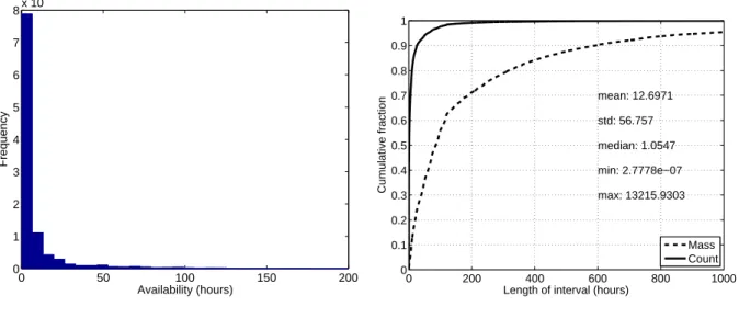
and the mass-count disparity (see Figures 2(a) and 2(b)).

We observe significant right skew. For example, the shortest

80% of the availability intervals contribute only about 10%

of the total fraction of availability. The remaining longest

20% of intervals contribute about 90% of the total fraction

Test

Runs std

Runs up/down

ACF

Kendall

All

# of hosts

101649

144656

109138

101462

57757

Fraction

0.602

0.857

0.647

0.601

0.342

Table 1. Result of Randomness Tests

of availability. The implication for modelling is that we

should focus on the larger availability intervals.

But which hosts can be modelled by which distributions

with which parameters?

7.0.1

Clustering Background

We use two standard clustering methods, in particular

k-means and hierarchical clustering, to cluster hosts by their

distribution. K-means randomly selects k cluster centers,

groups each point to the nearest cluster center, and repeats

until convergence. The advantage is that it is extremely fast.

The disadvantages are that it requires k to be specified a

pri-ori, the clustering results depend in part on the cluster

cen-ters chosen initially, and the algorithm may not converge.

Hierarchical clustering iteratively joins together the two

sub-clusters that are closest together in terms of the average

all-pairs distance. It starts with the individual data points

working its way up to a single cluster. The advantage of

this method is that one can visualize the distance of each

sub-cluster at different levels in the resulting dendrogram,

and that it is guaranteed to converge. The disadvantage is

that we found the method to be 150 times slower than

k-means.

7.0.2

Distance Metrics for Clustering

We tested several distance metrics for clustering, each

met-ric measures the distance between two CDFs [9].

Intu-itively, Kolmogorov-Smirnov determines the maximum

ab-solute distance between the two curves. Kuiper computes

the maximum distance above and below of two CDFs.

Cramer-von Mises finds the difference between the area

of under the two CDFs. Anderson-Darling is similar to

Cramer-von Mises, but has more weight on the tail.

Using these distance metrics is challenging when the

number of samples is too low or too high. In the former

case, we do not have enough data to have confidence in

the result. In the latter case, the metric will be too

sensi-tive. A model by definition is only an approximation. When

the number of samples is exceedingly high, the distance

re-ported by those metrics will be exceedingly high as well.

This is because the distance is often a multiplicative factor

of the number of samples.

Our situation is complicated even further by the fact that

we have a different number of samples per host. Ideally,

when computing each distance metric we should have the

same number of samples. Otherwise, the distance between

two hosts with 1000 samples will be incomparable to the

distance between two hosts with 100 samples.

Our solution is to select a fixed number of intervals from

each host at random. This method was used also in [7],

where the authors had the same issue. We also discussed

this issues with a statistician, who confirmed that this is an

acceptable approach.

However, if we choose the fixed number to be too high, it

will excluded too large of a portion of hosts from our

clus-tering. If we choose the number to be too low, we will not

have statistical confidence in the result. We choose the fixed

number to be 30 intervals as discussed in Section 6. The test

statistics corresponding to each distance metric is normally

distributed, and so with 30 intervals, one can compute

p-values with enough accuracy.

We performed extensive experiments to compare the

dis-tance metrics for several cases including for different

sub-sets of iid hosts. We also conducted positive and negative

control experiments where the cluster distributions were

generated and known a priori. The following conclusions

were been found to be consistent across all the cases

consid-ered. We found out that Kolmogorov-Smirnov and Kuiper

are not very sensitive in terms of distance as they are only

concerned with extreme bounds. Cramer-von Mises and

Anderson-Darling revealed that they are good candidates of

clustering, but Anderson-Darling is engaged with high time

and memory complexity. Moreover, Cramer-von Mises is

advantageous for right-skewed distributions [9]. Thus we

used the Cramer-von Mises as the distance metric when

clustering.

7.0.3

Cluster Results and Justification

We found that optimal number cluster was 6. We justify

this number of clusters through several means. First, we

ob-served the dendrogram as a result of hierarchical clustering

for a random subset of hosts (due to memory consumption

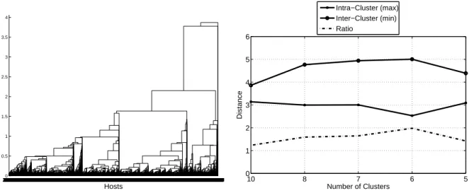
and scaling issues). As it can be seen in Figure 3(a) the tree

is an unbalanced tree where the height of tree shows the

dis-tance between different (sub)clusters. The good separation

of hosts in this figure confirmed the advantage of

Cramer-von Mises as the distance metric (in comparison to the

re-sult with other metrics). The number of distinct groups in

this dendrogram where the distance threshold is set to one

0

50

100

150

200

0

1

2

3

4

5

6

7

8

x 10

Availability (hours)

Frequency

(a) Histogram

0

200

400

600

800

1000

0

0.1

0.2

0.3

0.4

0.5

0.6

0.7

0.8

0.9

1

Length of interval (hours)

Cumulative fraction

mean: 12.6971

std: 56.757

median: 1.0547

min: 2.7778e−07

max: 13215.9303

Mass

Count

(b) Mass-count

Figure 2. Distribution of Availability Intervals

reveals that number of clusters should be between 5 to 10.

Second, using the result of hierarchical clustering as

a bootstrap, we run k-means clustering for all iid hosts

and then compute the within-group and between-group

dis-tances for various values of k (see Figure 3(b)). We observe

that the maximum ratio of inter-cluster over intra-cluster

distance is with six clusters. Specifically, for k of 6, the

inter-cluster distance between all clusters was maximized

relative to other values of k. Also, for k of 6, the distance

between all clusters is roughly equal (about 5).

Third, we plotted the EDF corresponding to each cluster

for a range of k. In this way, we can observe convergence

or or divergence of clusters during their formation.

Fourth, we plotted the EDF corresponding to each

clus-ter. Figure 4 shows good separation of these plots.

7.1

Parameter Estimation for Each

Clus-ter

After cluster discovery, we conduct parameter fitting for

various distributions, including the Exponential, Weibull,

Log-normal, Gamma, and Pareto. Parameter fitting was

conducted using maximum likelihood estimation (MLE).

Intuitively, MLE maximizes the log likelihood function that

the samples resulted from a distribution with certain

param-eters.

We also considered using moment matching instead of

MLE. However, because the overall distribution is heavily

right-skewed, we were concerned that moment matching,

which is relatively much faster then MLE, would not

pro-duce the most accurate results. Moment matching is also

0

200

400

600

800

1000

0

0.1

0.2

0.3

0.4

0.5

0.6

0.7

0.8

0.9

1

Availability (hours)

Cumulative fraction

1

4

2

5

3

6

Cluster 1

Cluster 2

Cluster 3

Cluster 4

Cluster 5

Cluster 6