Maintenance Planning for Circular Economy: Laundromat Washing Machines Case

(1)

HAL Id: hal-03151214

https://hal.archives-ouvertes.fr/hal-03151214

Submitted on 24 Feb 2021

HAL is a multi-disciplinary open access archive for the deposit and dissemination of sci-entific research documents, whether they are pub-lished or not. The documents may come from teaching and research institutions in France or abroad, or from public or private research centers.

L’archive ouverte pluridisciplinaire HAL, est destinée au dépôt et à la diffusion de documents scientifiques de niveau recherche, publiés ou non, émanant des établissements d’enseignement et de recherche français ou étrangers, des laboratoires publics ou privés.

Maintenance Planning for Circular Economy:

Laundromat Washing Machines Case

Ernest Foussard

To cite this version:

Ernest Foussard. Maintenance Planning for Circular Economy: Laundromat Washing Machines Case. [Technical Report] G-SCOP - Laboratoire des sciences pour la conception, l’optimisation et la pro-duction. 2021. �hal-03151214�

(2)

Technical report

MAINTENANCE PLANNING FOR

CIRCULAR ECONOMY: LAUNDROMAT

WASHING MACHINES CASE

February 24, 2021

Ernest Foussard Universit´e Grenoble-Alpes ernest.foussard@grenoble-inp.fr

(3)

2

Abstract

Circular Economy is at the heart of the new environmental policies in France, in Eu-rope and in the rest of the world. It consists in changing the global production apparatus such that its environmental footprint is minimized, by Reducing, Recovering, Recycling and Repurposing. Recent research emphasizes maintenance is one of the most effective tools to increase the lifespan of technical objects and thus minimizing interaction with the environment. Knowing this, the question is: How to efficiently schedule maintenance in order to improve the economic and environmental sustainability of a technical object? This work aims to provide tools for optimizing maintenance schedules within the frame-work of Circular Economy.

Based on a review of the literature on Circular Economy and Scheduling Theory, we present a Multi-Objective Mixed Integer Linear Program (MILP) for optimizing main-tenance planning alongside with a heuristic approach. Then, the specific application case of Laundromat washing machines is studied. Experiments are then realized and the results are presented and analyzed. Circular economy aware production/maintenance plannings are obtained for specific weightings of the objectives and provide decent re-sults even on large instances, yet some specific cases yield mixed rere-sults and potential improvements and further developments are suggested.

Keywords—Maintenance planning, Circular Economy, Functional Economy, Scheduling, Multi-Objective Optimization

(4)

3

Acknowledgements

This work has been supported by the French National Research Agency under the "In-vestissements d’avenir” program (ANR-15-IDEX-02) through the Cross Disciplinary Program CIRCULAR and has been completed at the laboratory G-SCOP, under the direction of Marie-Laure Espinouse and Margaux Nattaf, as part of the M2 ORCO curriculum of the Grenoble-Alpes University.

(5)

4 CONTENTS

1 Introduction

For centuries, economy in Europe has been based on a "linear model": extract, produce, consume and thrash, which corresponds to the usual division of the economy in three sec-tors. With the endlessly growing demand of raw materials and the raise of the awareness regarding environmental concerns, it is necessary to find and implement alternatives to the linear model of production. Indeed, in 2019, humanity consumed 1.8 times the quantity of resources that the Earth can generate in one year. On top of that, the problem of greenhouse gases emissions and waste generation has become more and more concerning and question our way of producing and living. Plus, due to its strong dependency to raw materials, this model of production induces geopolitical tensions and social issues in some regions of the world such as Middle East or South America. Economically speaking, this system is not ideal either, as economical actors could do substantial cuts in the expenditure for raw materials by adopting more sustainable production policies. For all of these reasons, it is not compatible with the objectives of sustainable development and not viable in the long run.

Circular Economy is one of the alternatives to the linear system of production. According to the Ellen McArthur Foundation, which is one of the main authorities is this field, the goal of Circular Economy is to decouple economy from the environment, by keeping products in use within a closed loop and thus reducing resource extraction, waste generation and pollution. Recent policies in France and in Europe [Min] aim for a fully sustainable economical model and introduce the transition to a Circular Economy as one the main focus for years to come.

Functional economy is one among the various school of thought that make up Circular Economy. Instead of selling a product, manufacturers sell the service tied to the product. The direct consequence is that the more durable the product is, the most profitable it is to the manufacturer. Currently, in linear economy, the strategy of planned obsolescence allows the manufacturer to increase the demand and thus increase its profits at the expense of the customers and the environment. As the goal of functional economy is to make the product more durable, maintenance has an important role to play in it, and more generaly in circular economy. In the broadest sense, maintenance denotes any operation which can be com-pleted to increase the lifespan of a product already in use. Maintenance planning has been widely studied in the field of optimization, yet within this framework, brand-new objectives and constraints appear and have to be handled.

In this work, methods for maintenance planning within the functional economy paradigm are presented and assessed on a typical application case: laundromat washing machine. At first, new constraints and objectives coming from of circular, and more specifically functional, economy are identified. Then, a maintenance planning problem embedding them is defined and a multi-objective mixed-integer linear programming (MILP) model is proposed, with variants and improvements, as well as a heuristic approach. Finally, the problem is solved, performances are analysed and the model is discussed in light of the results. Section 2 is a lit-erature review on circular economy, maintenance planning and previous operations research results for sustainable development. Section 3 introduces and states the problem. In section 4, the MILP model is presented along with some notable properties and a heuristic algorithm.

(7)

6 2 STATE-OF-THE-ART

In Section 5 an experimental protocol for assessing the model is suggested and executed, the results are discussed and analyzed. Finally, Section 6 concludes this work and presents new challenges and perspectives for this subject. In appendix A, some complementary informa-tion about the context of the internship and a personal review is provided, and appendix B contains a table summing up the notations of the problem.

2 State-of-the-art

2.1 Circular Economy

Circular economy (CE) is currently not a clearly defined concept [KRH17]: due to the ab-sence of global consensus on the definition between academics, policymakers and economic actors, there is a large variety of definitions and understandings of CE which results in the vagueness of the actual concept.

The Ellen MacArthur foundation provides the most often cited and most known defini-tion [Ell], which emphasizes the idea of decoupling the economical growth from the resource consumption with three key principles in mind: designing waste and pollution out, keeping products and materials in use, and regenerating natural systems.

According to [Die17, Ell13], CE can be divided into a few major schools of thought, each of them provides a paradigm and guidelines to implement it in the industry:

• Functional Economy [Sta05] focuses on optimizing the "use" of goods and services, and thus the management of the existing wealth. This results in a shift from a producer/con-sumer paradigm towards a provider/user paradigm. Typically, the producer remains the owner of the product, and rather lends the product or sells a service with it. This school of thought is usually presented as the contrary of planned obsolescence since the more reliable the system and easy to maintain the system is, the more lucrative it will be. • Biomimicry consists in designing industrial processes by taking inspiration from the

natural trophic network: plants convert minerals from the ground into organic matter and energy, herbivores consume plants, carnivores consume herbivores. At each step of this cycle, organic matter is rejected into the ground. This organic matter is consumed by the decomposers, which turn it back into minerals that can be consumed again veg-etals and so on [Die17]. In the linear model, primary, secondary and ternary sectors can be respectively assimilated to vegetals, herbivores and carnivores. Yet, for the loop to be complete, it lacks decomposers. Hence, biomimicry approaches usually address this issue by finding placeholders for decomposers. It is the starting point of the following schools of thought.

• Regenerative Design [Col12] takes inspiration from permaculture, with a systems theory-based approach: the processes themselves renew or regenerate the source of energy and materials they consume. In the same way, each actor of the tropic network con-tributes to the global harmony of the ecosystem, economic actors creates positive

(8)

im-2.2 Sustainability in Operations Research 7

pacts (rather than doing less damage) from which the other actors of the system can then benefit.

• Industrial Ecology (IE) consists in studying the flows of energy and materials through industrial systems [AA02]. The fundamental statement of IE is that society and econ-omy are bounded within the biosphere and cannot exist outside of it. This is different from the traditional three pillars description of sustainable development (usually rep-resented with a Lewis diagram), as, in this framework, environment encompasses the two other pillars. With this in mind, industrial ecology analyses industrial systems and their interactions with each other, the society and the environment.

• Cradle-to-Cradle (C2C) is a new theory which was introduced by McDonough and Braun-gart in 2010 with the book Cradle to Cradle: Remaking the Way We Make Things [Ell15, MB10]. They stated that even the most basic industry products contain unnecessary hazardous and noxious products, and that products should be designed in such a way they are not harmful: even recycling, or "downcycling" as they call it, is not viable as it often results in a waste of energy, and after a few cycles, the product itself becomes a waste. C2C gets rid of the notion of waste and replaces it by the notion of nutrient, which can be of two types: either natural, in which case it can safely be returned to the nature after being used, or technical. A technical nutrient must be designed in such a way that it can be kept forever in use (see Figure 1). Their book itself is made of synthetic materials which can then be "upcycled" later to make new books, and this process can be repeated forever with minimal waste of energy.

All these approaches aim at transforming the current model of production into a more sustainable and more environment compatible one. In this study, the maintenance planning problem is addressed from a functional economy point of view.

2.2 Sustainability in Operations Research

With the apparition of new legislations and new expectations from customers, compa-nies and industry have been pushed to adapt and change their policies in order to match the social and environmental objectives of sustainable development and circular economy. Thus, new problems with new objectives and new constraints have appeared and have been addressed lately in the field of Operations Research to take up this challenge. Sustainable de-velopment, green logistics, reverse logistics, closed-loop supply chain are recurrent themes in the recent operations research literature and are closely tied to the challenges of circular economy [SAB20].

A literature review of operations research methods for a sustainable supply chain is pre-sented in [BPdSC18]. A vast majority of these methods deal with strategic-level decisions. Most of the methods are based on mathematical programming and usually focus on the eco-nomic and environmental pillars while only few articles deal with the social pillar. The envi-ronmental awareness of the models is in the majority of the cases implemented by using

(9)

en-8 2 STATE-OF-THE-ART

Figure 1: Circular Economy from a C2C point of view [Ell13]

ergy consumption and CO2emissions as objectives to minimize or as constraints, few

meth-ods also focus on waste generation.

Sustainable manufacturing has also been extensively covered in the scheduling literature . Reviews are available in [GTP15] and [AI18]. Most of the problems covered are addressed with MILP modeling and are mainly solved using heuristics or solvers to a lesser extent. The most recurrent environmental factors is electric power consumption by far, either as a constraint or an objective. Other factors include greenhouse gas emissions, water consumption, reuse and waste, or the availability of the system.

Various operations research methods have been developed for assessing sustainability and life-cycles of products. A literature review is available in [TKSS19].

While sustainability is a very recurrent theme in operations research papers, the circu-lar economy is an emerging subject and has yet to be explored in details [Tsi18, PNS19]. In [SAB20], a state-of-art review of the applications of circular economy to production planning and the new challenges and opportunities are presented. Yet, to the best of our knowledge, the problem of maintenance planning within circular economy has not been treated in the operations research literature.

(10)

2.3 Maintenance planning 9

2.3 Maintenance planning

Maintenance is one of the main tools available to improve the sustainability of a techni-cal object. Any operation which aims at increasing the lifespan or the reliability of a system falls under the preventive maintenance category. Some of the circular economy paradigms presented before, especially functional economy are built around the concept of preventive maintenance to improve the lifespan of product. It can consist of operations ranging from cleaning to the total replacement of a component. Of course, the former usually has a smaller economic and environmental cost than the latter. Hence, the choice of which type of mainte-nance has to be planned and is critical when it comes to optimizing the durability of a prod-uct. A division in seven categories of preventive maintenance policies for one-unit systems is proposed in [Wan02]: age-dependent, periodic, sequential, failure limit, repair limit, repair counting limit and reference time policies. The scheduling approaches presented bellow fall mostly under the periodic, sequential or age-dependent categories.

A first approach consists in enriching classical production planning problems by intro-ducing periodic preventive maintenance periods as constraints. With this approach, fail-ures rates are kept low by the fact that recurrent maintenance operations are scheduled. In [RAAH14], the problem of minimizing the weighted sum of maximum earliness and maxi-mum tardiness on a single machine with such maintenance periods is addressed. In the for-mulation of the problem, a maximum duration between two preventive maintenance is in-cluded. The problem is proven to be NP-hard, and a heuristic method using approximations algorithms for bin-packing is provided by the authors for large instances of the problem. The periodic preventive maintenance policy is also considered in [WCC13] with the problem of minimizing the makespan on multiple machines. The NP-hardness of the problem is stated, and a genetic algorithm is proposed.

Maintenance planning on unrelated machines with deterioration effect has been studied in [GAFE16, FGAE+_{17]. With some specific objective functions and under the assumption}

that maintenance resets a machine to its initial state, the problem can be reduced to solving a set of Assignment Problems of polynomial-size in the number of tasks. Regarding the circular economy, the assumption on maintenance resetting machines is too strong, as one may not want or be able to fully regenerate the machine in practice.

A recurrent theme in the literature is the problem of preventive maintenance of machines subject to age-dependent stochastic failure rates. In [BFNG16], a cost-minimization model under quality constraints with such failure rates is presented. In this approach, time is divided in large periods, and maintenance can only be scheduled at the beginning of a period. This is justified by the fact that usually, in the industrial context, preventive maintenance cannot be planned at any time, but only under certain occasions where it may not impact productivity e.g. weekends or vacations. The problem is modeled as a non-linear optimization problem, and several metaheuristic approaches are proposed by the authors.

Similarly, in [MU11], the case of a single machine with multiple components and two types of maintenance operations, repairing or replacing a component, has also been studied. In particular, a reliability objective function has been proposed. The components are also sub-ject to an increasing stochastic failure rate as their age increases. Maintenance operations

(11)

10 3 PROBLEM

reset or reduce the effective age of a component, and hence reduce the failure rate of it. The problem is modeled with mixed integer linear programs and is then reformulated as dynamic programs. A mixed method involving both dynamic programming and branch and bounds algorithm is used to solve them in a reasonable amount of time. In [CLP14], the problem of finding robust production/maintenance schedules for a single machine subject to increasing failure uncertainty is addressed. A joint model is given and NP-hardness of the resolution is proved. The problem is then solved using a heuristic method.

In [MMA12], a method is proposed to include preventive maintenance on production schedules for problems with multiple machines by evaluating failure and repair rates. A non-linear optimization model for the problem of minimizing the total system unavailability is presented and solved using neighborhood search techniques.

2.4 Case of Laundromat washing machines

The washing machine case is a recurrent example in the circular economy literature [DBT+_20,

Die17]. From a user perspective, a washing machine is a technical object with multiple com-ponents and multiple possible failure modes. As most household appliances, multiple main-tenance operations are possible and completed during its long lifespan (usually more than 10 years). Washing machines have also been subject to planned obsolescence lately. Hence, it is relevant to address this issue from a functional economy perspective to provide viable alter-native economic models. Data, from repair operators, on failure modes and average lifespan of the components of washing machines is presented in [TAM19]. In [Die17], extra details on the life cycle of some components are also presented.

Laundromat washing machines are the typical case of the functional economy, as instead of the machine itself, it is the service of washing clothes which is sold. In the following, the general term of "production" is used to designate the machine when it is available for use.

3 Problem

The maintenance policies of the problem presented in this work belongs to the age-dependent category. Notable state-of-the-art features used in this problem include equipment health level [NDP19], multiple components machine and modeling of the evolution of the wear of the components by a recurrence equation, partial repair [MU11], energy consumption and waste generation based objective [BPdSC18].

The goal of the problem is to find the most satisfying planning of production and main-tenance for a machine with multiple components concerning the criteria of the circular econ-omy. In the case of washing machines, the components can be e.g. electronic circuits, solenoid valve, drum etc. Each component has a wear level, which has a direct incidence on the envi-ronmental and economical cost of production and may eventually disable the machine when too high. Maintenance operations can affect one or multiple components, may or may not require to immobilize the machine, and also have an environmental and economic cost to reflect for example the cost of an intervention by a specialized technician, the amount of

(12)

3.1 Machine and components 11

raw materials consumed to repair or replace a component, the quantity of noxious materi-als released, etc. On washing machines, such operations can range from cleaning the filter to changing components. Finally, the end of life policies are also taken into account, as compo-nents in decent shape can be sold, repurposed or recycled for example.

The notations of the problem are recapped in Table 3 in appendix A.

3.1 Machine and components

A single machine with G components is considered, with a set of M possible maintenance operations. In the notations, components and maintenance are respectively denoted by the exponents g and m. Each maintenance operation can be repeated multiple times, but its efficiency may decay each time it is completed. The time horizon is denoted by T and is large enough to encapsulate the whole lifespan of the machine while keeping a decent time sampling. Time periods are denoted by the index t.

The wear level of a component is denoted by W_tg and ranges from zero to one: zero corre-sponds to the like-new condition, while one correcorre-sponds to the unusable state. Maintenance restore one or multiple components by an amount based on the reference regeneration rate

REGg m, also ranging from zero to one. Depending on the context and the model, one may opt for either a fixed or decaying amount of regeneration per maintenance. A fixed amount is closer to an ideal Cradle-to-Cradle scenario, in which the technical object is made in such a way that it can be repaired forever. Decaying maintenance efficiency, in the contrary, ap-plies to objects which were not specifically purposed to last forever, but can still be repaired multiple times before being completely unusable.

The machine can be either in production or maintenance mode. In the case of the produc-tion mode, a fixed revenue EPP per time period as well as a resource cost depending on the wear level of components fc(Wt) (where Wtdenotes the the vector of dimension G of the wear

level of each component at time step t). The wear level of each component g also increases by a degradation value DVg. For the sake of simplicity, it is assumed that the amount of noxious wastes generated during a production cycle is negligible in comparison to the other environ-mental factors, thus no waste cost is charged for production periods. In maintenance mode, up to Mmax can occur simultaneously. Each maintenance has a starting date and an immo-bilization duration dm(which can be zero). Plus, a resource cost RCm, a waste cost W Cmand an economic cost ECm _{are charged for each maintenance.}

The end-of-life of the machine also has to be treated: choosing when the exploitation of the machine stops and in which state is an important part of the decision-making. Depend-ing on the wear level of the components some economic profit can be made from repurpos-ing, recycling or selling the components. Some hazardous wastes may also be released in the environment. This phenomenon is captured by the respective functions GBEOL(WT) for the

(13)

12 4 MODELING AND SOLVING

3.2 Objectives

Aside from the usual economic objective, three more objectives are taken into considera-tion.

The lifespan of the machine has to be maximised. This corresponds to the idea that in a proper Circular Economy, technical objects should be kept as long as possible in the technical cycle, or even forever according to the Cradle-to-Cradle school of thought. The functional economy framework adds another dimension to this objective, which is the availability of the machine, and thus, the quality of the service.

The resource inputs have to be minimized. These notably include the amount of energy and water consumed, and the quantity of raw materials extracted.

Wastes in the broadest sense also have to be minimized. This not only include noxious materials rejected in the nature, but also CO2emissions and sewage. Any waste counts: for

example, if a component of the machine is replaced, not only the wastes from releasing the old component has to be taken into account, but also the wastes generated during the manu-facturing of the new component, during extraction and refining of the raw materials etc. This statement is also true for the resource inputs.

4 Modeling and Solving

A multi-objective mixed integer linear program for solving this problem and first solutions for small data sets are detailed in this section.

4.1 Model

In the model below, it is assumed that the various functions fc, GWEOL and GBEOL are

affine functions. In particular, the following notation is used fc(Wt) = PG_{g =1}(AgW_tg+ Bg). The

main hypothesis of the model is that the exploitation of the machine stops before the time horizon is reached, and thus, the benefits and wastes generated at the end-of-life are com-puted based on the wear level when the time horizon is reached. Therefore, the machine can also be in idle mode to have feasible solutions.

4.1.1 Decision variables

The decision variables of the model are presented in the table below:

Decision

variable Domain Meaning and interpretation

x_tm {0,1} Boolean variable equal to 1 if a maintenance of type m starts at time t, 0 otherwise.

(14)

4.1 Model 13

C_tg R+ Represents the resource cost induced if the machine is in

pro-duction mode at time step t.

W_tg R+ Wear level of the component g at the time step t. W_{the corresponding vector of dimension G for all component at}t denotes

time step t.

Table 1: Decision variables of the model

4.1.2 Objectives

There are two types of resource inputs: the resource consumption while the machine is producing C_tg (decision variable which depends on the wear level of the machine) and the amount of resources consumed when one maintenance operation is done.

mi n RESOU RC ES = XG g =1 T X t=0 C_tg₊ XM m=1 T X t=0 xm_t RCm (1)

We assume that when the machine is producing, no noxious nor hazardous wastes is re-jected in the environment. Therefore, the waste outputs are the wastes generated by mainte-nance and when the machine is trashed.

mi n W AST ES = M X m=1 T X t=0 xm_t W Cm+GWEOL(WT) (2)

Finally, the economic cost is composed of the expenses for maintaining the machine, the profit from exploiting, recycling or disassembling the machine and selling the pieces.

mi n COST = XM m=1 T X t=0 ECmxm_t ₋XT t=0 EPP pt−GBEOL(WT) (3)

An extra objective, LI F ESPAN is considered, and represents the availability of the ma-chine. It is expressed as the number of periods of production of the mama-chine. A noticeable fact is that one of the terms of the objective COST , PT_t=0EPP ptis proportional to LI F ESPAN ,

meaning that COST is affinely dependent on LI F ESPAN . However, both objectives are rele-vant and represent two different things: LI F ESPAN can be seen as the availability and qual-ity of the service, while COST purely deals with the profitabilqual-ity of it. Both are correlated, yet prioritizing one or the other may drastically change the shape of a solution.

max LI F ESPAN =XT

t=0

(15)

This first formulation is quite simplistic, other formulations involving more parameters could be considered.

4.1.3 Constraints

The constraints (5) and (6) enforce that no production should occur while a machine is im-mobilized due to maintenance. This also takes into account the case of maintenance which do not require any immobilization time for the machine: in this case, dm must be equal to 0. The expression of these constraints is derived from the expression of the Cumulative con-straint in temporal linearizations of the Resource-Constrained Project Scheduling Problem, as proposed by Bonifas in [Bon17].

PM

m=1Ptτ=max(0,t−dm₊₁₎x_τm≤ Mmax ∀t ∈ {0..T } (5)

Pt

τ=max(0,t−dm₊₁₎x_τm≤ 1 − pt ∀t ∈ {0..T } ∀m ∈ {1..M} (6)

Constraint (7) implies all wear levels must be inferior to 1, which means that production is possible only if at the end of the period, the wear level of all of the components would be inferior to 1.

W_tg _{≤ 1 ∀t ∈ {0..T } ∀g ∈ {1..G}} (7) Constraint (8) describes the evolution of the wear level of the components over time.

W_t+1g _{≥ W}_tg_{+ p}tDVg− P_m=1M REGg mxm_t ∀t ∈ {0..T } ∀g ∈ {1..G} (8)

Notice that if DVg is dependent on the wear level of the components, then constraint (8) is no longer linear. A linear formulation for this specific case is provided in Section 4.1.5. Most of the time, this inequality behaves as an equality. Putting an inequality instead allows to plan maintenance even when the regeneration value is higher than the wear level for at least one of components. In this case, the wear level is expected to reach zero after the maintenance due to the constraint on the non-negativity of the decision variable W_tg.

Constraint (9) linearizes the expression of the resource inputs, by introducing the auxiliary variable C_tg which represents the quantity of resources consumed by production for the time step t, with K1= maxg ∈{1..G}Ag

C_tg _{≥ A}g_{· (1 −W}_tg) + Bgpt− K1(1 − pt) ∀g ∈ {1..G}, ∀t ∈ {0..T } (9)

Constraint (10) initializes the wear level of the components to 0 at the first time period.

(16)

4.1 Model 15

Constraints (11) and (12) state the domains of the decision variables.

x_tm, pt∈ {0,1} ∀m ∈ {1..M}, ∀t ∈ {0..T } (11)

Ct,Wtg≥ 0 ∀g ∈ {1..G}, ∀t ∈ {0..T } (12)

Finally, the complete expression of the MILP is the following:

mi n RESOU RC ES = XG g =1 T X t=0 C_tg₊ XM m=1 T X t=0 xm_t RCm (1) mi n W AST ES = M X m=1 T X t=0 xm_t W Cm_+GWEOL(WT) (2) mi n COST = M X m=1 T X t=0 ECmxm_t ₋ T X t=0 EPP pt−GBEOL(WT) (3) max LI F ESPAN = T X t=0 pt (4) subject to: XM m=1 t X τ=max(0,t−dm₊₁₎ xm_τ _{≤ M}max _{∀t ∈ {0..T }} (5) t X τ=max(0,t−dm₊₁₎ x_τm≤ 1 − pt ∀t ∈ {0..T } ∀m ∈ {1..M} (6) W_tg _{≤ 1 ∀t ∈ {0..T }} _{∀g ∈ {1..G}} (7) W_t+1g _{≥ W}_tg_{+ p}tDVg− M X m=1 REGg mx_tm _{∀t ∈ {0..T }} _{∀g ∈ {1..G}} (8) C_tg _{≥ A}g_{· (1 −W}_tg) + Bgpt− K1(1 − pt) ∀g ∈ {1..G} ∀t ∈ {0..T } (9) W₀g = 0 ∀g ∈ {1..G} (10) xm_t , pt ∈ {0,1} ∀m ∈ {1..M} ∀t ∈ {0..T } (11) Ct,W_tg ≥ 0 ∀g ∈ {1..G} ∀t ∈ {0..T } (12) 4.1.4 Symmetry-breaking cut

With the model defined above, at any time period t, the machine may be either in produc-tion mode, maintenance mode or idle mode, i.e. neither producing nor being maintained.

(17)

Assuming that in an optimal solution of this program, there are I idle periods, these can be placed anywhere in the schedule without any impact on the objectives.

In practice, this does not make sense: a washing machine of a Laundromat is never set idle for a few periods at a random point in time before being exploited again. However, having idle periods at the end of the planning does makes sense, as this means that it is no longer worth to exploit the machine with regards to the objective, and therefore the machine has reached its end of life state and can be, in a Circular Economy context, salvaged or repurposed.

The other problem is that, as the location of these idle periods have no impact on the objectives, a lot of symmetries appear due to this issue, which results in increasing drastically the computation time for solving it. (see Section 5.2)

The two following sets of constraints are introduced to force idle periods at the end of the schedule.

p_t+1_{≤ p}t+ Pt_τ=t−dm₊₁xm_t ∀t ∈ {0..T } (13)

xm_t+1≤ pt+ Pt_τ=t−dm₊₁xm_t ∀t ∈ {0..T } ∀m ∈ {1..M} (14)

Constraint (13) states that if the machine was neither producing nor being maintained at time period t, then it cannot produce at time period t +1. Constraint (14) does the same with each maintenance operation.

4.1.5 Case of wear-dependent degradation rate

If the degradation rate depends on the wear level of the components, a linear formula-tion of the equaformula-tion (8) is obtained by replacing it by the equaformula-tion (15), an auxiliary variable

ζt∈ R+, representing the value of the production pt and DVg(Wt) is introduced, and the

con-straints (16), (17) and (18) are also added. The expression of the "big M" constant K2is the

following: K2= maxg ∈{1..G}maxv∈[0,1]gDVg(v)

W_t+1g ≥ Wtg+ ζt− P_m=1M REGg mxmt ∀t ∈ {0..T } ∀g ∈ {1..G} (15)

ζt ≤ K2pt ∀t ∈ {0..T } (16)

ζt≤ DVg(Wt) ∀t ∈ {0..T } ∀g ∈ {1..G} (17)

ζt ≥ DVg(Wt) − (1 − pt)K2 ∀t ∈ {0..T } ∀g ∈ {1..G} (18)

This set of constraints introduces another "Big M" constraint, and therefore drastically increases the complexity of the problem. Generating relevant degradation values in a complex task, thus, due to a lack of time, this has not been investigated further.

(18)

4.1 Model 17

4.1.6 Formulations for maintenance efficiency decay

The basic formulation of the problem and the corresponding model both have a few issues in practice. Some of them are exposed in Section 5.2. The main lacking feature is the loss of efficiency of the maintenance as the components are repaired, meaning that eventually the machine has been worn and repaired so much that it may not be possible to exploit and repair it any longer. This problem is addressed by two different means in this section.

4.1.6.1 "Decaying Maintenance" (DM) formulation

The "Decaying Maintenance" formulation is a broader model and consists in introducing a new piece of data, MDFg m_{, which represents a fixed degradation rate per maintenance and}

component of the regeneration rate. Then the constraint (8) is reformulated as follows:

W_t+1g _{≥ W}_tg_{+ p}tDVg− PM_m=1¡REGg m− MDFg mPt−1_τ=0x_τm¢x_tm ∀t ∈ {0..T } ∀g ∈ {1..G}

(19) This equation cannot be linearized using the usual methods for linearizing the product of a boolean variable and a real number, since there, the quantity REGg m_{− MDF}g mPt

τ=0xmτ

can become negative. For example, in the case of one component and one maintenance, which initially regenerates by 1 and loses 0.4 every time it is used. The third time this main-tenance is used, it would regenerate the component by 0.2, and the efficiency of the mainte-nance would drop to −0.2. At this point, it is no longer worth to realize this maintemainte-nance, yet the value of REGg m_{− MDF}g mPt

τ=0xτmis negative.

Thus, by replacing with max(0,REGg m_−MDFg mPt

τ=0xτm), one should be able to express

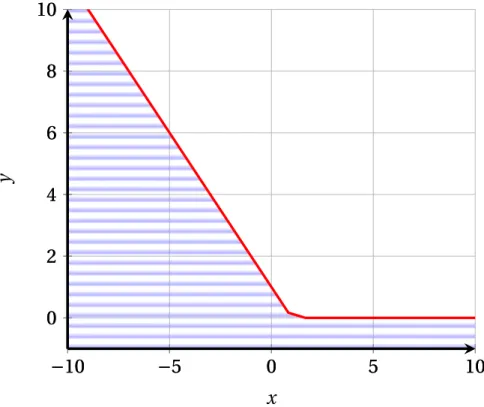
Constraint (19) as a set of linear constraints, assuming that the max function could be lin-earized later on. Yet, with this new expression, Constraint (19) would no longer be convex, therefore no linearization is possible, as illustrated in Figure 2.

Therefore, the usual methods for Mixed Integer modeling and solving cannot be applied in this case. Other methods to overcome this issue could be investigated in further develop-ments.

4.1.6.2 "Limited Maintenance" (LM) formulation

While the "Decaying Maintenance" formulation focuses on the constraint (8) by replacing

REGg mby a decision variable, the "Limited Maintenance" consists in introducing precedence chains of maintenance operations of decreasing efficiency.

This model introduces a new piece of data PREC which represents the precedence con-straints on the maintenance operations as the set of arcs of a graph. It is assumed that in the graph G = (M ,PREC), where M is the set of maintenance operations, the degree of the vertices is at most 2, and there are no cycles.

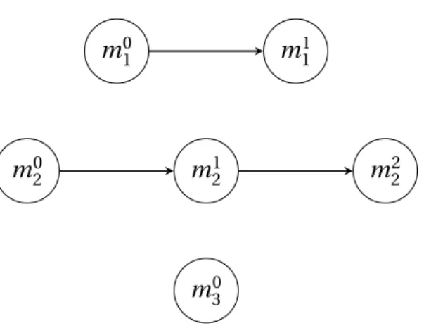
As a matter of illustration, let us consider an instance of the DM formulation for a one component machine, such that, three maintenance types are available (M = 3), named re-spectively m1, m2and m3with the following regeneration rates and maintenance decaying

(19)

−10

−5

0

5

10

0

2

4

6

8

10 −10

−5

0

5

10

0

2

4

6

8

10 x

y

(20)

4.1 Model 19 m0 1 m11 m0 2 m21 m22 m0 3

Figure 3: Precedence graph of the example in Section 4.1.6.2

factors: REG = [0.6,0.5,0.3] and MDF = [0.4,0.2,0.3]. In the corresponding LM formulation,

m2would be converted in three unit maintenance operations m0₁, m1₁, m2₁with respective

re-generation rates 0.5, 0.3 and 0.1. By doing the same on the other maintenance, the new model ends up with M0_{= 6, and the precedence graph of Figure (3)}

Constraint (20) states that the successor of a maintenance operation may only be sched-uled if its predecessor has been schedsched-uled.

PT

t=0xmsucc ≤ PT_t=0xmpr ed ∀(msucc,mpr ed) ∈ PREC (20)

Constraint (21) implies that a maintenance operation cannot occur as long as its prede-cessor has not been completed:

PT t=0t xmsucc− PT_t=0t xmpr ed ≥ dmpr ed· P T t=0xmpr ed− T · (1 − P T t=0xmpr ed) ∀msucc,mpr ed∈ PREC (21) Constraint (22) implies that, each maintenance operation cannot occur more than once: Indeed, in this formulation, maintenance operations which can be scheduled multiple times are replaced by precedence chains of unit maintenance operations.

PT

t=0xmt≤ 1 ∀m ∈ {1..M} (22)

This model is not a broader formulation of the initial model, in particular, it does not cover cases where the regeneration rate does not decrease since it would require infinite chains of maintenance. This formulation has been tested, compared with the other methods and ultimately assessed in Section 5.2.

Overall, due to the limitations of the DM formulation, the case of mixed problems with both fixed maintenance rate and maintenance that decay over time are not covered by the scope of this work. A new model could be designed for these cases, mixing both categories a maintenance operations: those which efficiency decays over time and those for which the efficiency remains constant.

(21)

4.2 Notable properties and results

4.2.1 Complexity of the model

This model, with no symmetry breaking nor LM, has (M + 1) · (T + 1) binary variables and 2GT real variables, which is a considerable amount given that T needs to be a very large num-ber in order to get relevant results. For example, given that one can expect a "fair" washing machine to be working for at least 20 years, sampling periods of one day would require T to be equal to at least 7300.

The number of constraints is quite substantial as well: 5+G+T +M(T +1)+3G(T +1). More specifically, some constraints drastically increase the complexity of the model: constraint (5) makes this problem enter the field of cumulative scheduling, which are known to be computa-tionally hard problems [GJ79]. Plus, such temporal linearization are usually not very efficient according to Bonifas in [Bon17]. Constraint (9) is a "big M" constraint and increase substan-tially the time complexity of the resolution of this mixed integer linear program.

With the LM formulation, 2 · |PREC| + M0_{≤ 3 · M}0_{constraints are added, the variable M is}

replaced by M0_{which increases the size of the problem. M is a lower bound on M}0_{, but M}0_has

no upper bound: when the loss of efficiency of maintenance operations becomes closer to 0,

M0_{diverges to infinity. Plus, the introduction of chains of optional maintenance operations}

arguably increases the complexity of the problem, and heavily cripples the resolution speed. The problem is multi-objective, and so is the model. At first, a weighted sum of the objec-tive is considered: wrRESOU RC ES + wwW AST ES − wlLI F ESPAN + wcCOST .

4.2.2 Upper bound on Lifespan

The bounds of the objectives is a very useful information to have for balancing the weights for each objectives. The two following sections provide such bounds for all of the objectives.

In this section, an upper bound on the lifespan for the case where each maintenance can be scheduled only once in the planning horizon is presented. The following lemma gives this upper bound.

Lemma 4.1. Assuming that each maintenance can only occur once, i.e. the phenomenon of maintenance efficiency decay is captured by modeling each maintenance type as a precedence chain of single-use maintenance operations. The following inequality is verified:

LI F ESPAN ≤ ming ∈{1..G}$ 1 +P M

m=1REGg ,m

DVg

%

Proof. For the sake of the simplicity of the proof, it is assumed the wear level is defined for t > T and remains stationary. Therefore ∀t ≥ T,Wtg = WTg. Considering the constraint (8),

which has the following expression:

(22)

4.2 Notable properties and results 21

Then, by summing over the time periods, the following inequality is obtained:

PT

t=0(Wt+1g −W g

t ) + Pm=1M REGg mPTt=0xmt ≥ PTt=0ptDVg ∀t ∈ {0..T } ∀g ∈ {1..G} (23)

And then, by telescopic cancellation and since under the "limited maintenance" hypoth-esis, ∀m ∈ {1..M} PT_t=0xm_t ≤ 1:

W_Tg_−W₀g_{+ P}M_m=1REGg m_{≥ DV}gPT

t=0pt ∀t ∈ {0..T } ∀g ∈ {1..G} (24)

By definition of LI F ESPAN , and since W₀g = 0 and W_Tg ≤ 1:

1 + PM_m=1REGg m_{≥ DV}g_{· LI F ESPAN ∀t ∈ {0..T } ∀g ∈ {1..G}} (25) And therefore, since ∀g ∈ {1..G},DVg ≥ 0:

LI F ESPAN ≤1+Pm=1M REGg m

DVg ∀t ∈ {0..T } ∀g ∈ {1..G} (26)

By integrality of LI F ESPAN , and since this equation is true for all g :

LI F ESPAN ≤ ming ∈{1..G}$ 1 +P M

m=1REGg ,m

DVg

%

As a side note, this result can be generalized in the case where there exists a component g such that W₀g _{6= 0. In this case:}

LI F ESPAN ≤ ming ∈{1..G}$ 1 −W g

0 + Pm=1M REGg ,m

DVg

%

The question of the equality for max LI F ESPAN is still open. The bound is denoted

U BLI F ESPAN for the rest of the report.

4.2.3 Other bounds

Having rough bounds on each objective is useful to determine their magnitudes, and com-pute relevant weights for the objective aggregation. Upper and lower bounds for each objec-tive are provided in the table below.

Aside from the LI F ESPAN upper bound, these bounds have been computed by studying every term that composes the objectives. Zero is the lower bound of both RESOU RC ES and

LI F ESPAN since all the terms of these objectives are positive. Plus, equality is reached when

(23)

the same scenario. Since Equation (2) is composed of two terms, the first one P_m=1M PT

t=0xmt W Cm

is positive and equal to 0 when no maintenance operations are planned. The second term

GWEOL(WT) is minimized when the wear level is minimized, hence the bound. Finally, the

cost lower bound is also computed by taking lower bounds of each the terms: the cost of maintenance operations is equal to 0 when there are no maintenance operations. The profit from producing is maximised when the number of periods of production is maximised, and the profit from end of life policies is maximised when all the components end up in a like-new state. Notice that this bound is not necessarily reachable.

All the upper bounds aside from U BLI F ESPAN have been computed following the same

guidelines. The costs on the objectives related to maintenance are maximised when all avail-able maintenance are scheduled. In the case of RESOU RC ES, the environmental cost of production depends on the wear level of the components (see Equation (1). The cost due to this term of the objective is roughly bounded by maximum possible cost for each time peri-ods. In the case of W AST ES and COST , the end-of-life costs and wastes are maximized when the wear level is equal to 1 for every component. Again, these bounds may not necessarily be reachable.

Objective Lower bound Upper bound

RESOU RC ES 0 PM

m=1RCm+ (T + 1) · fc(1G)

W AST ES GWEOL(0G) PM_m=1W Cm+GWEOL(1G)

LI F ESPAN 0 _{mi n}_{g ∈{1..G}}¹1−W0g+PMm=1REGg ,m

DVg

º

COST _{−EPP ·UB}LI F ESPAN−GBEOL(0G) −GBEOL(1G) + PM_m=1ECm

Table 2: Bounds on the objectives

4.3 Heuristic for MIP start

As explained before, MIP solving is a very costly operation, and in the case of this problem with large instances, it may not be possible to solve it with a reasonable amount of time or space. MIP start consists in initializing the solver with an already known good bound, there-fore reducing the search space significantly. A heuristic algorithm, detailed below, was de-signed to find such bound.

The algorithm consists of three steps: a first solution is built greedily regardless of the weights of each objective. This first step prioritizes the lifespan. Then, by shifting the main-tenance, the objectives RESOU RC ES and COST are improved without any trade-off with

LI F ESPAN . Finally, the best time period, with regards to the aggregation of the objectives,

for stopping the exploitation of the machine is chosen. The heuristic is presented bellow us-ing the LM formulation and hypothesis, it can be easily adapted for either the initial model or the DM formulation.

(24)

4.3 Heuristic for MIP start 23 0 5 10 15 20 25 30 0 0.2 0.4 0.6 0.8 1 Time step t W ear le ve lW

Evolution of the wear level

0 5 10 15 20 25 30 0 0.2 0.4 0.6 0.8 1 Time step t W ear le ve lW

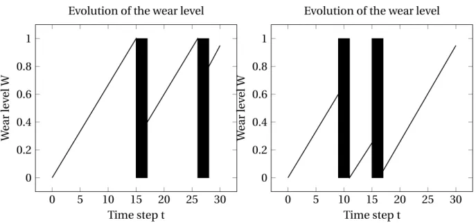
Figure 4: Initial and second steps of the heuristic

4.3.1 Initial feasible solution

The first step consists in building a first feasible solution constructively by producing whenever possible and scheduling a maintenance whenever production is no longer possi-ble, as detailed in Algorithm 1. This first step provides at first a very good solution with regard to the LI F ESPAN objective. For each component, maintenance operations are ordered in a priority queue from the most efficient to the less efficient. The efficiency criterion of a main-tenance operation with respect to a component is non-trivial to define as soon as there are multiple components, therefore multiple criteria are possible.

The retained criterion in this work is "Highest Regeneration Rate First", that is, mainte-nance are sorted by decreasing order of the ratio of the regeneration rate divided by the du-ration of immobilization. This criterion is good with regards to lifespan and easy to compute, however, it does not take both environmental and economic costs into account.

Other criteria can be better depending on the situation, such as the cost efficiency ra-tio or the environmental impact. Yet, these can result in the loss of some regenerara-tion, or choose maintenance with very long immobilization time, which may not necessarily be cost-effective.

Assuming the priority queues are based on Fibonacci heaps, with a deletion operation has a time complexity of O(log (n)) [FT87], and since the complexity of operation consisting building the queues is O(GMlog (M)) complexity of this first step is O(TGlog (G)+GMlog(M)). 4.3.2 Maintenance left shift

The next step consists in, starting from the end of the planning, moving each maintenance period a few time periods earlier as long as no regeneration is lost in the process: Constraint

(25)

Entries:An instance of the problem; Maintenance priority queues (Qg)_{g ∈{1..G}} Result:A feasible production/maintenance schedule

Initialization:Wear level variables W_tg, production variables pt, maintenance

variables x_tmare initialized to 0.

t ← 0;

/* Iteration on each time period */

whilet < T do

/* Computation of the potential wear increase of the components */

Compute Kg_{= W}_tg_{+ DV}g _{∀g ∈ {1..G} ;}

/* Check if production is possible at this step */

if_{∀g ∈ {1..G} K}g _{≤ 1 then}

/* Production is possible, a production period is scheduled */

pt ← 1 ;

W_t+1g ← Kg ∀g ∈ {1..G} ;

t ← t + 1

else

/* Production is not possible due to component g , the best

corresponding maintenance operation is scheduled */

Choose any g such that Kg_{> 1 ;}

m ← Pull(Qg) ;

Remove m from all the queues ;

xm_t _{← 1;}

/* Time index jumps to the end of the maintenance operation */

t ← t + dm_;

end end

(26)

25

(8) is an inequality rather than equality. This allows to schedule maintenance operations which would regenerate some components to a negative wear level, putting the component in like-new condition, but also means that some of the regeneration is wasted, and therefore more efficient use of the maintenance could be done. In this algorithm, these situations are avoided as much as possible.

During a first pass, maintenance periods are identified with their starting and ending dates. Then, starting from the earliest maintenance period, the operation Shift Left as de-scribed in Algorithm 2 as applied as long as the current maintenance period does not intersect with another one and the following condition is verified. Otherwise, the algorithm continues with the next maintenance period:

∀t ∈ {d − 1, f − 1} Wtg− DVg≥ 0

Entries:An instance of the problem and a feasible schedule

A maintenance period starting at time d and ending at time f ; Result:A better feasible production/maintenance schedule

for_{t ← d − 1 to f − 1 do}

W_tg_{← W}_tg_{− DV}g _{∀g ∈ {1..G} ;} xm

t−1← xmt ∀m ∈ {1..M} ;

end

Algorithm 2:Operation Shift Left

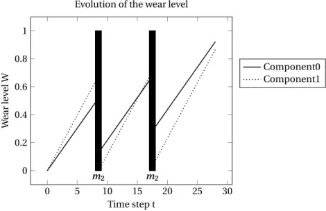
The operation Shift Left has a time complexity of O(M +G), therefore, the time complexity of the whole step is O(T (M + G)). Both steps are illustrated for one component and some arbitrary data in Figure 4: the graph of the wear level is represented with maintenance periods materialized as black rectangles.

4.3.3 End-of-life setting

The final step consists in evaluating the value of the objectives at each time period as-suming that the exploitation of the machine stops there. From there, the best time period to stop exploiting the machine is determined and all periods coming after are replaced with idle periods. This step is detailed in 3 and illustrated in Figure 5.

This last step has a time complexity of O(T (M +G)).

5 Experimentations

To assess the model presented previously, an experimental protocol was conceived and implemented. In this section, the protocol is presented in details, and then some of the results are presented.

(27)

26 5 EXPERIMENTATIONS 0 5 10 15 20 25 30 0 0.2 0.4 0.6 0.8 1 Time step t W ear le ve lW

Figure 5: Last step of the heuristic

Entries:A feasible schedule S of the problem ;

Result:A better feasible production/maintenance schedule fort ← 0 to T do

Ob j ecti vet ← EvaluateOb j ecti ve(S, t);

end

best_ti me ← ar gmint∈{0,T }(Ob j ecti vet);

for_{t ← best_time to T do}

pt← 0;

xm_t _{← 0 ∀m ∈ {1..M} ;}

W_tg_{← W}_{best_ti me}g _{∀g ∈ {1..G} ;}

end

(28)

5.1 Experimental protocol 27

5.1 Experimental protocol

The protocol consists in building a large panel of artificial data sets based on real data whenever possible, and arbitrarily chosen otherwise. This aims at testing the behavior of the model on typical real-life scenarios. The next step consists of running the model with different parameters on each of these instances.

5.1.1 Data sets generation

To simplify and limit ourselves to a reasonable number of experiments, the following as-sumptions are made: maintenance operations cannot be scheduled in parallel and the related immobilization time is one time period. The number of components is equal to the number of available maintenance. A more exhaustive testing protocol could be considered later.

First, the most interesting parameters to vary have been identified. The number of time periods T , which can be seen as a sampling frequency of the time horizon, is a critical pa-rameter as the choice of its value results in a trade-off between the accuracy of the solution and the computation time required to find the optimum. Therefore, multiple values for this parameter are tested: 30, 60, 120 and 360. The number of components G, and thus the num-ber of maintenance operations M, is also an interesting parameter to vary. Based on the data from repair operators [TAM19] and from [Die17], a set of five critical components of washing machines was selected: the solenoid valve, the electronic control card, the pumps, the heater and the drain system. The data sets involve either 1, 2 or 5 of these components.

The other parameters either do not have a significant impact on the size or the nature of the problem, therefore, these have been computed to the greatest extent possible on real data available, packed with some randomness. When it was not possible to so, the values have been set arbitrarily while making sure that the order of magnitude is reasonable enough to not overshadow the other parameters.

Time-dependent data is calibrated in such a way that the time horizon represents a 30 years long time period. In [TAM19], the average age of a washing machine undergoing re-pair services for each defective component is provided. The degradation rate DVg of each component is computed based on these two previous statements.

To the best of our knowledge, no precise data on the economic cost, resources consumed and waste generated per maintenance is available. Thus, the order of magnitude of the eco-nomic cost is estimated roughly to thousands of euros, by taking into account salary costs and potential travel and transportation expenses. Arbitrarily, the value ECm is given by a nor-mal distribution of mean 2000 and standard deviation 400. Due to the lack of data, resources consumed RCm and waste generated W Cm are also given by this distribution.

Regeneration values REGg mand maintenance decay factor MDFg mare generated using normal distributions. The maintenance focus primarily on one component and slightly re-generate the others. The value for the main component is centered around 0.6, while it is 0.3 for the others. The same is done with the maintenance decay factor MDFg m, centered around 0.2 for the main component and 0.1 for the others.

(29)

typi-28 5 EXPERIMENTATIONS

cal laundromat of Grenoble: 5eper wash and assuming that the machine is used ten times per day. The resource consumption function captures both the energy and the water consump-tion of the machine and is converted in euros to be comparable with the other quantities of the problem. An A+++-class washing machine consumes 0.8kW h of energy and 50L of water per cycle. The energy cost of water supply represents approximately 5kW h/m3[FD12], there-fore the total energy consumption is 11kW h/d ay. Since the electricity cost is 0.15e/kW h and the water cost is 2.92e/m3in the region of Grenoble, the retained values for this affine function are 1.7e/d ay when the appliance is new, and it is assumed that this value doubles when all the components are fully worn.

Finally, for the end-of-life affine functions, the economical benefit GBEOL is computed

based on the prices of new and second-hand professional washing machines, respectively ranging from 2000€ and 15000€, and from 1000€ to 5000€. The exact values are determined by random draws of uniform distribution. The same distribution has been chosen arbitrarily to compute the end-of-life waste generation function GWEOL. With multiple components,

the values of the three affine functions presented before are divided equally between each component.

5.1.2 Protocol

The model is tested for both mono-objective and multi-objective situations. Mono-objective situations are obtained by setting the weight to 1 for only one of the objectives, and 0 for the others. This is done for each of the objectives. For multi-objective situations, two sets of weights for the linear aggregation of the objectives are tested: an environmental aware scenario where the lifespan of the machine, the amount of resources consumed and waste generated are prioritized, and an economic aware scenario where the economic cost is pri-oritized over the other objectives. The upper bound and the lower bound of each objective are computed using the results presented in Section 4.2. Then, the weight of each objective is computed as the product of the amplitudes of variation of the other objectives. All the weights are then divided by the smallest one, to make sure the solver does not manipulate excessively large numbers. Finally, some objectives are prioritized by multiplying their weights by 100. This system of weights has some limitation, as only takes into account the magnitude of the objectives without considering the average value. Therefore, due to the multiplicative effect of the weights, off-centered objectives may be magnified.

For each of these situations, four configurations are tested.

1. Baseline model with the symmetry-breaking cut;

2. "Limited maintenance" model without the symmetry-breaking cut;

3. "Limited maintenance" model with the symmetry-breaking cut;

4. "Limited maintenance" model with symmetry breaking and MIP start using the heuris-tic presented before.

(30)

5.2 Analysis of the results 29

Each of these configurations are designated bellow by the corresponding number.

The models have been implemented using IBM ILOG CPLEX Optimization Studio 12.9.0. All the experiments were done on a laptop running on Windows 10 Professional edition, with 8 GB of RAM and one Intel Core i5-3210M 2.50 GHz processor (4 cores). A time limit of one hour per experiment is set.

5.1.3 Extraction and visualization

For each experiment, the values of the decision variables representing production periods

pt, scheduled maintenance operations x_tmand the evolution of wear level of each component

are collected. The value of each objective, as well as the gap and the computation time, are also extracted. The production/maintenance schedule of the solution is represented on the graph of the evolution of wear level: maintenance operations are represented as black rectan-gles which cover the whole immobilization duration.

5.2 Analysis of the results

In this section, some of the results of the experimentations are presented and discussed. As the heuristic could not be implemented and tested in time, the experimental protocol has not been fully completed and does not include the MIP start scenario. In the first subsection, the results for the mono-objective case are presented and discussed, and then the limits are identified. The same is done with the multi-objective case in the second subsection. Finally, conclusions are drawn about both models and their relevance with regards to the problem.

5.2.1 Mono-objective case

Looking at the mono-objective case first provides interesting insights on some of the ex-treme behaviors of the model, and allow to assess some parts of the model. For example, one can look at the results when only the economical objective is active, and compare it to real situations of the linear economy. In this section, we focus on the smallest instances of the problem, which are enough to discern the main behaviors of the mono-objective, while limiting the visual clutter on the various figures.

The case of wastes or resources minimization is not represented in the figures below, since in the optimal solution, neither production nor maintenance occur at any point in time, the machine remains idle. This is the expected behavior, as, without any economic or social pur-pose, there is no point to produce from a purely environmental perspective. In this model, keeping the machine idle for the whole time does lead a solution with a minimum value for

RESOU RC ES of 0, and a minimum value for W AST ES equal to GWEOL(0G). These objective

are interesting only when combined with the two others.

The economic cost objective provides interesting information about the behaviour of the model. Firstly, one may notice that it seems to encourage the lifespan maximisation, which is expected since the economic profit from producing is proportional to the lifespan of the machine. This component of the objective seems to be dominating in this case: the number of

(31)

30 5 EXPERIMENTATIONS 0 5 10 15 20 25 30 0 0.2 0.4 0.6 0.8 1 m1 m1 Time step t W ear le ve lW

0 5 10 15 20 25 30 0 0.2 0.4 0.6 0.8 1 m1 m1 Time step t W ear le ve lW

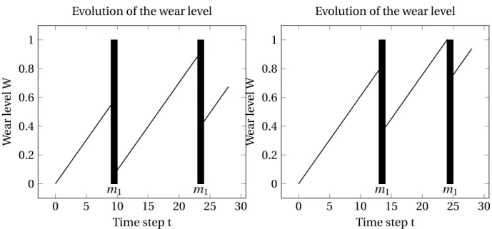
Figure 6: Mono-objective results for an instance with T = 30 and G = M = 1 On the left: Cost minimization. On the right: Lifespan maximization.

maintenance operations is the minimum required to be able to produce until the time horizon

T is reached. The machine is discarded with a high level of wear, which means that profit from

the end-of-life policies is low.

Finally, the lifespan maximization behavior resembles the economic cost minimization one, but an irregularity at the end can be observed. Since Constraint (8) is an inequality, which is intended to work as an equality at the exception of some very specific situations, the wear level does not represent what the real wear level should be, as in the last maintenance, the full potential of regeneration is not used. This does not occur when this objective is used in conjunction with another one, since the other objectives penalize higher wear levels.

The results with the LM formulation of the same instances as previously are represented in Figure 7. A noticeable change is these instance do no longer present a sort of periodic regime since the unique maintenance type has a decaying regeneration rate.

Again, the solutions prioritizing only the resources and wastes minimization objective re-main consist in not producing at all, which is the intended behavior. With the lifespan alone, the same unrealistic behavior due to the inequality in Constraint (8) is observed. This time it manifests as a steeper slope for the duration of the 25th time period, resulting with a higher wear level than reality.

Some interesting statements can be made when looking at the case of cost minimization: First, all possible maintenance operations are planned to keep the wear level at the end of the resolution as low as possible and generate more benefits from repurposing and selling spare parts for example. Yet, the wear level is not kept as low as possible at all times. For example, the second maintenance could have taken place earlier, but since the wear level does not impact any economical cost aside from the end-of-life benefits, there is does not have any impact on the objective. Overall, maintenance operations are scheduled regularly

(32)

5.2 Analysis of the results 31 0 5 10 15 20 25 30 0 0.2 0.4 0.6 0.8 1 m1 m1 m1m1 Time step t W ear le ve lW

0 5 10 15 20 25 30 0 0.2 0.4 0.6 0.8 1 m1 mm23m4 Time step t W ear le ve lW

Figure 7: Mono-objective results for an instance with T = 30 and G = M = 1 On the left: Cost minimization. On the right: Lifespan Maximisation

to make sure more benefit is done from having more production periods and a better end-of-life return on investment, which, aside from the end-end-of-life, looks very similar to a typical linear economy policy: get the most economical benefit from the machine, and then discard it.

Performance-wise, it is required to look at larger instances, as these small instances are all solved in less than a second. The instance used has a sample size of 120, with 5 components and 5 maintenance.

In the case of the baseline model, resources and wastes minimization problem are solved to optimality almost instantaneously. The lifespan problem and the economic cost problem are solved quickly in 0.05s. For the LM case, the trivial cases of resources and wastes mini-mization are solved to optimality respectively in less than 0.02 and 0.27 seconds. The lifespan minimization problem is solved to optimality in 7.83s, while after one hour of solving, we only get a solution with a gap of 1.77%. One may notice already the drastic raise in computation time for lifespan and even more for the economic cost.

As a conclusion of this section, only the economic cost objective is relevant alone. The other objectives should always be used in conjunction with another one, especially in the case of LI F ESPAN , for which absurd solutions are eliminated by symmetry breaking as soon as another objective is used, even with a very small weight.

With more than one component, similar behaviors are observed. Previous experiments with larger time horizons and higher degradation rates have allowed to

Overall, the economic cost and lifespan objective have a constructive effect, encouraging to have more production periods sustained by maintenance operations, while the resources and wastes objectives have the opposite effects. The multi-objective case should therefore be a trade-off between these two extremes.