HAL Id: hal-03240308
https://hal.archives-ouvertes.fr/hal-03240308
Submitted on 28 May 2021
HAL is a multi-disciplinary open access
archive for the deposit and dissemination of
sci-entific research documents, whether they are
pub-lished or not. The documents may come from
teaching and research institutions in France or
abroad, or from public or private research centers.
L’archive ouverte pluridisciplinaire HAL, est
destinée au dépôt et à la diffusion de documents
scientifiques de niveau recherche, publiés ou non,
émanant des établissements d’enseignement et de
recherche français ou étrangers, des laboratoires
publics ou privés.
Dynamic aware aging design of a simple distributed
energy system: A comparative approach with single
stage design strategies
Hugo Radet, Xavier Roboam, Bruno Sareni, Rémy Rigo-Mariani
To cite this version:
Hugo Radet, Xavier Roboam, Bruno Sareni, Rémy Rigo-Mariani. Dynamic aware aging design of a
simple distributed energy system: A comparative approach with single stage design strategies.
Renew-able and SustainRenew-able Energy Reviews, Elsevier, 2021, 147, pp.111104. �10.1016/j.rser.2021.111104�.
�hal-03240308�
Highlights
Dynamic aware aging design of a simple distributed energy system: a comparative approach
with single stage design strategies.
Hugo Radet,Xavier Roboam,Bruno Sareni,Rémy Rigo-Mariani
• Implementation of a multi-time scale model where the interaction between investment and operation is taken into account for the design of energy systems.
• Introduction of a generic framework (common simulator referential) to compare and to assess the performances of different design strategies.
• Comparison of the aging aware approach with more standard methods based on single equivalent years, in terms of cost and computational performances.
• Sensitivity analysis with regard to different energy prices and constraint for the system self-sufficiency (i.e. minimum import of energy from the upstream grid).
Dynamic aware aging design of a simple distributed energy system:
a comparative approach with single stage design strategies.
Hugo
Radet
a,∗,
Xavier
Roboam
a,
Bruno
Sareni
aand
Rémy
Rigo-Mariani
b aLAPLACE, Univ. Toulouse, CNRS, INPT, Toulouse, FrancebG2Elab, Univ. Grenoble Alpes, CNRS, INPG, Grenoble, France
A R T I C L E I N F O
Keywords:
Distributed energy system Aging
Multi-time scale model Techno-economic
Mixed-integer-linear-programming (MILP)
A B S T R A C T
This paper focuses on the integrated management and design of a distributed energy systems (DES) with solar generation and energy storage. The DES remains voluntary simple as the ob-jective is to focus on the design methodologies rather than the system complexity. The article aims at bridging the gap between conventional DES design strategies, made in a single stage fashion over a representative period, and expansion planning problems that perform dynamic sizing over decades with oversimplifications of the system operations. Especially, the paper investigates to what extent the value of the model is increased when aging is controlled over the system lifetime compared to standard methods based on a single equivalent year. To ad-dress these questions, a multi-time scale model is first implemented by coupling both the DES operation and the sizing. The optimal asset capacities are computed in the form of a dynamic in-vestment plan over the system lifetime that can accommodate potential changes in energy prices or cost of technology. Then, the results are compared with single stage design strategies on a common simulation framework. The implemented multi-time scale planning displays good performances with up to 20% cost reduction compared to typical single stage designs. Finally, the impact of the energy rates and system self-sufficiency are investigated. The obtained results show that significant investments in energy storage arise for electricity prices multiplied by three compared to the baseline or with strong self-sufficiency constraint over 60%.
1. Introduction
The integration of renewable energy sources into conventional systems has been extensively addressed in the past two decades with the need for reduced carbon emissions and in order to tackle the limitation of fossil fuels. In particular, the concept of Distributed Energy System (DES) has emerged and highlights the resources connected closer to the end-user and the implementation of local energy management strategies with both generation and consumption on site. The integrated management and design of DES have then been widely investigated and is oftentimes expressed in the form of optimization problems which minimize a trade-off between the operating costs and the capital expenditures [1]. Different optimization architectures are considered in the literature with (i) “all in one” approaches where sizing and operating parameters are variables of a single optimization problem [2,3] and (ii) bi-level optimizations with an inner loop that simulates the system operation and an outer loop (usually metaheuristics) that investigates different system configurations (i.e. type and size of assets) [4,5].
The main challenge of such problems is to tackle the mathematical complexity and the necessity to avoid prohibitive computational times, especially due to the need to simulate the system operation over long time horizons before finding the optimal configuration. In order to ensure tractability, the problems are usually simplified by means of linearization techniques or mixed integer linear programming (MILP) as in [2,3]. Also, the systems are often simulated over reduced periods of time from sets of typical days up to a whole year at the maximum with hourly or half hourly time steps [6,7,8,9], in order to represent the daily, weekly and seasonal variations for the loads and renewable based generation. The equivalent annualized cost (EAC) becomes the criteria to minimize and is assumed to be constant over the system lifespan (typically decades). Thus, most of the reviewed DES studies fail to capture the longer term variabilities that may impact the energy prices and cost of technologies (e.g. over decades). Most importantly, the DES are oftentimes designed in a single stage fashion at the beginning of the system lifetime and the optimal sizes of the equipment are expressed as a unique vector. In case the DES includes technologies with lifespans shorter than the study
∗Corresponding author:
radet@laplace.univ-tlse.fr(H. Radet)
ORCID(s):
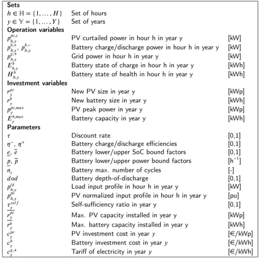
Sets
ℎ∈ ℍ = {1, … , 𝐻} Set of hours
𝑦∈ 𝕐 = {1, … , 𝑌 } Set of years Operation variables
𝑝𝑝𝑣,𝑐ℎ,𝑦 PV curtailed power in hour h in year y [kW]
𝑝𝑏,+ ℎ,𝑦, 𝑝
𝑏,−
ℎ,𝑦 Battery charge/discharge power in hour h in year y [kW] 𝑝𝑔,+
ℎ,𝑦 Grid power in hour h in year y [kW] 𝐸𝑏
ℎ,𝑦 Battery state of charge in hour h in year y [kWh] 𝐻𝑏
ℎ,𝑦 Battery state of health in hour h in year y [kWh]
Investment variables
𝑟𝑝𝑣
𝑦 New PV size in year y [kWp]
𝑟𝑏
𝑦 New battery size in year y [kWh] 𝑝𝑝𝑣,𝑚𝑎𝑥
𝑦 PV peak power in year y [kWp]
𝐸𝑏,𝑚𝑎𝑥
𝑦 Battery capacity in year y [kWh]
Parameters
𝜏 Discount rate [0,1]
𝜂−, 𝜂+ Battery charge/discharge efficiencies [0,1]
𝑒, 𝑒 Battery lower/upper SoC bound factors [0,1]
𝑝, 𝑝 Battery lower/upper power bound factors [h−1]
𝑛𝑐 Battery max. number of cycles [-]
𝑑𝑜𝑑 Battery depth-of-discharge [0,1]
𝑝𝑙𝑑
ℎ,𝑦 Load input profile in hour h in year y [kW] 𝑝𝑝𝑣
ℎ,𝑦 PV normalized input profile in hour h in year y [pu] 𝜏𝑠𝑒𝑙𝑓
𝑦 Self-sufficiency ratio in year y [0,1] 𝑟𝑝𝑣𝑦 Max. PV capacity installed in year y [kWp] 𝑟𝑏
𝑦 Max. battery capacity installed in year y [kWh] 𝑐𝑝𝑣
𝑦 PV investment cost in year 𝑦 [e/kWp] 𝑐𝑏
𝑦 Battery investment cost in year 𝑦 [e/kWh] 𝑐𝑔,+
𝑦 Tariff of electricity in year 𝑦 [e/kWh]
Table 1 Nomenclature
horizon (e.g. batteries), replacements are taken into account with extrapolation built upon a single simulated year and integrated in the economic analysis a posteriori. Typically, the assets are replaced with the same capacities, regardless the potential evolution of input parameters over time such as energy prices, equipment costs and load profiles.
On the other hand, for longer term design, expansion planning studies encountered in the literature correspond to problems where the installation and decommissioning of power plants are investigated over several decades (up to 50 years) at a national scale with the cost of technologies updated over time [10]. However, expansion planning problems often consider oversimplifications of the system operations with limited snapshots or monthly averages which may not be relevant if high shares of intermittent renewable energy production are considered. The authors in [11] and [12] implemented a formulation that integrates multiple time-scales to tackle this latter issue. However, the interaction between investment and operation is not fully captured, i.e. the way systems are operated has no consequences on their aging, thus the number of replacements over the horizon does not depend on the operation (the lifetime of systems are usually fixed a priori to their calendar lifetime). This simple trick makes the implementation easier as it is known beforehand when the assets have to be decommissioned, but it is not fully relevant when storage technologies are included in the DES as the number of charge/discharge cycles has great consequences on the equipment lifetime [13,
14].
This paper addresses the aforementioned shortcomings by bridging the gap between the different time scales which is deemed necessary to represent the DES lifetime in the design phase, from hourly variations to years ahead prediction for energy prices and cost of technologies. The main challenge tackled by the paper is to investigate to what extent the value of the model is increased when aging is controlled in the DES design phase compared to standard methods based on a single equivalent year. To address this question, a multi-time scale model is formulated for a simple case
study consisting of a consumer, a solar generator and a battery. The DES remains voluntary simple as the objective is to focus on the methodology and the novelties given by this approach rather than the system complexity. Applying the proposed methodology to more complex DES is definitely the intended direction of future works. The optimal sizing of the system is not expressed as a single vector any longer but as a dynamic investment plan. The article also proposes a reproducible methodology in order to assess the performances of the implemented strategy compared to conventional single stage optimizations. This is allowed by a generic benchmark that simulates the system operation along its lifetime, once the design plan is defined. This common simulator referential, may or may not embed the same profiles and parameters as the ones considered in the design phase. The objective is to provide a common framework in order to equally discriminate different planning strategies which is not commonly encountered in the literature. To summarize, the main contributions of this work are:
• Implementation of a multi-time scale model where the interaction between investment and operation is taken into account for the design of energy systems.
• Introduction of a generic framework (common simulator referential) to compare and to assess the performances of the different design strategies.
• Comparison of the aging aware approach with more standard methods based on single equivalent years, in terms of cost and computational performances.
• Sensitivity analysis with regard to different energy prices and constraint for the system self-sufficiency (i.e. minimum import of energy from the upstream grid).
The paper is organized as follows: section2shows the problem formulation of the multi-time scale model and the optimization problem statement. Then, section3describes the resolution methods which are going to be compared. Next, the assessment strategy is introduced in section4. Finally, results are shown in section5, conclusions and perspectives are drawn in section6.
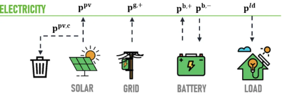
Figure 1: Schematic view of the DES with solar panels and a battery.
2. Mathematical formulation
This section describes the fundamental mathematical equations that allow modeling the DES operation and the impact of investment choices. The presented problem formulation will be considered as the common simulator ref-erential when different design strategies are further discriminated. Note that the design problem will embed similar equations and time series profiles. This strong assumption would be equivalent to a long term deterministic design with “perfect foresight” and no modeling errors. The authors remind that the objective here is to provide a common frame-work in order to appropriately discriminate different design strategies. Considering the uncertainties for the energy prices, equipment cost or load profiles right from the design phase is not in the scope of this paper. The formulation is then based on [15] applied to the design and operation of the DES. Both the investment and operation dynamics are included into a common optimization problem as described in the following. Note that the main difference with [15] is the comparison of the aware-aging model with other design strategies depicted in section3. To this end, the current paper is first limited to the deterministic case. This latter hypothesis is further discussed in section6.
2.1. Notations
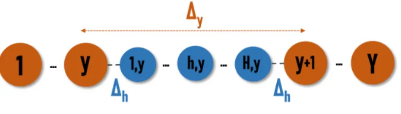
The investment dynamic is a slow process compared to the operation where power flow decisions need to be made every hour. Hence, we define two time scales with the set of years 𝑦 ∈ 𝕐 = {1, … , 𝑌 } and hours ℎ ∈ ℍ = {1, … , 𝐻} with Δ𝑦and Δℎ the two time steps respectively. A time continuum is ensured as depicted in figure 2. Investment
decisions are made along the set 𝕐 (orange nodes) while the operations along both sets 𝕐 and ℍ (blue nodes).
Figure 2: A time continuum is ensured in the simulation between the investment (𝑦) and operating (ℎ) time scale
2.2. Operation time-scale
At the operation time-scale, the decision variables are the charged/discharged power in the battery 𝑝𝑏,−
ℎ,𝑦, 𝑝 𝑏,+
ℎ,𝑦 and
the curtailed solar power 𝑝𝑝𝑣,𝑐
ℎ,𝑦. Their limits are represented by constraints (1), (2) and (3). 𝑝 and 𝑝 are the maximum
discharging/charging c-rate respectively, which limit the power exchanged by the battery. The grid power 𝑝𝑔,+
ℎ,𝑦 is
introduced to make the optimization implementation clearer. This flow is represented as a mathematical variable but does not correspond to any physical degree of freedom for the problem. This latter quantity is also limited (4) by the maximum power allowed by the external network.
0≤ 𝑝𝑝𝑣,𝑐ℎ,𝑦 ≤ 𝑝𝑝𝑣,𝑚𝑎𝑥 𝑦 ⋅ 𝑝 𝑝𝑣 ℎ,𝑦 (1) 0≤ 𝑝𝑏,ℎ,𝑦+≤ 𝑝 ⋅ 𝐸𝑦𝑏,𝑚𝑎𝑥 (2) 0≤ 𝑝𝑏,ℎ,𝑦−≤ 𝑝 ⋅ 𝐸𝑦𝑏,𝑚𝑎𝑥 (3) 0≤ 𝑝𝑔,ℎ,𝑦+≤ 𝑔 (4)
State variables are the battery state of charge (SoC) and state of health (SoH), both of them expressed in kWh here (i.e. available kWh for the SoC and remaining usable kWh for the SoH). The SoC dynamic is given by equation (5) where
𝜂−and 𝜂+are respectively, the charging and discharging efficiencies. In order to limit the battery degradation due to
deep charge and discharge, the SoC has to remain between upper and lower bounds (usually set to 80% and 20% of the battery capacity, respectively) as it is commonly done for Li-ion batteries (6).
𝐸ℎ𝑏+1,𝑦= 𝐸ℎ,𝑦𝑏 + (𝜂−⋅ 𝑝𝑏,−
ℎ,𝑦−
𝑝𝑏,ℎ,𝑦+
𝜂+ )⋅ Δℎ (5)
𝑒⋅ 𝐸𝑦𝑏,𝑚𝑎𝑥≤ 𝐸𝑏ℎ,𝑦≤ 𝑒 ⋅ 𝐸𝑦𝑏,𝑚𝑎𝑥 (6)
The battery SoH is computed using a simple model (7) based on the maximum exchangeable energy during its lifespan [13]. This model only considers aging due to cycling. Calendar aging mostly depends on the ambient temperature conditions [16], thus we assume that the temperature is controlled in order to neglect this latter contribution. Further-more, battery parameters such as loss of capacity or increased internal resistance over time are not taken into account. As in [13], the maximum exchangeable energy depends on the battery maximum number of cycles 𝑛𝑐for a fixed
depth-of-discharge 𝑑𝑜𝑑. The battery is replaced whenever the SoH reaches zero. Thus, its value has to remain positive all along the simulated horizon (8).
0≤ 𝐻ℎ,𝑦𝑏 ≤ 2 ⋅ 𝑛𝑐⋅ 𝑑𝑜𝑑 ⋅ 𝐸𝑏,𝑚𝑎𝑥𝑦 (8)
Then, the power balance is ensured by (9) where 𝑝𝑙𝑑
ℎ,𝑦is the power demand and 𝑝 𝑝𝑣
ℎ,𝑦is the PV normalized input profile
multiplied by the PV peak power 𝑝𝑝𝑣,𝑚𝑎𝑥 𝑦 .
𝑝𝑔,ℎ,𝑦++ 𝑝𝑝𝑣,𝑚𝑎𝑥𝑦 ⋅ 𝑝𝑝𝑣ℎ,𝑦− 𝑝ℎ,𝑦𝑝𝑣,𝑐+ 𝑝𝑏,ℎ,𝑦+− 𝑝𝑏,ℎ,𝑦−= 𝑝𝑙𝑑ℎ,𝑦 (9) Finally, a constraint on the self-sufficiency 𝜏𝑠𝑒𝑙𝑓
𝑦 ∈ [0, 1]is given by (10). The self-sufficiency represents the degree
of autonomy for the considered system. It is usually estimated as the share of local consumption supplied by the local generation and can be computed while considering the amount of energy imported from the upstream grid: a ratio equal to 1 means that all the electricity consumed is provided by the installed solar panels [17].
𝐻 ∑ ℎ=1 (𝑝𝑔,ℎ,𝑦+⋅ Δℎ)≤ (1 − 𝜏𝑦𝑠𝑒𝑙𝑓)⋅ 𝐻 ∑ ℎ=1 (𝑝𝑙𝑑ℎ,𝑦⋅ Δℎ) (10)
2.3. Investment time-scale
At the investment time scale, the decision variables are the new capacity installed for the battery 𝑟𝑏
𝑦and the new peak
power 𝑟𝑝𝑣
𝑦 for solar panels that could be made every year. They are both continuous, positive and bounded variables
(11), (12).
0≤ 𝑟𝑝𝑣𝑦 ≤ 𝑟𝑝𝑣 (11)
0≤ 𝑟𝑏𝑦≤ 𝑟𝑏 (12)
In order to properly model the replacement dynamic, a difference is made between the new design of systems and the existing system sizes which have to be updated when investment decisions are made. Thus, unlike single stage investment optimization, state variables are also introduced for the investment. Technology sizes could be increased or downscaled depending on the case study. Note that systems are assumed to be completely replaced when an invest-ment decision is made. Hence, system sizes 𝐸𝑏,𝑚𝑎𝑥
𝑦 and 𝑝
𝑝𝑣,𝑚𝑎𝑥
𝑦 need to be updated with the new installed capacities.
Otherwise, they remain the same as the year before. This investment dynamic is given by (13) and (14). Because solar panels aging is not considered in the current study, a linear formulation would have been possible for the investment dynamic of the PV. As it has little consequences on computational times, this generic formulation was adopted in the paper. 𝑝𝑝𝑣,𝑚𝑎𝑥 𝑦+1 = { 𝑟𝑝𝑣𝑦 ,if 𝑟𝑝𝑣𝑦 >0 𝑝𝑝𝑣,𝑚𝑎𝑥𝑦 ,otherwise (13) 𝐸𝑏,𝑚𝑎𝑥 𝑦+1 = { 𝑟𝑏𝑦 ,if 𝑟𝑏𝑦>0 𝐸𝑦𝑏,𝑚𝑎𝑥 ,otherwise (14)
2.4. Bridging the gap between time-scales
Both operation and investment decisions have to be made over the two time scales horizon. In order to ensure the inter-year continuity for the battery SoC and the SoH, the decision process is defined as follows: investment decisions are made at the end of the last hour of each year (𝐻, 𝑦) when the SoH and SoC are completely known over the year.
𝐸1,𝑦+1𝑏 = { 𝑒⋅ 𝑟𝑏 𝑦 ,if 𝑟𝑏𝑦>0 𝐸𝐻𝑏+1,𝑦 ,otherwise (15) 𝐻1,𝑦+1𝑏 = { 2⋅ 𝑛𝑐⋅ 𝑑𝑜𝑑 ⋅ 𝑟𝑏𝑦 ,if 𝑟 𝑏 𝑦>0 𝐻𝐻𝑏+1,𝑦 ,otherwise (16)
The capacities of the assets are then updated with the new sizes at the beginning of the first hour of the next year (1, 𝑦 + 1). Furthermore, any newly installed battery is assumed to be fully charged and with a maximum exchangeable energy (i.e. maximum SoH). Thus, continuity equations for the SoH and SoC between years are given by (15) and (16).
Finally 𝑢𝑦= (𝑝 𝑏,− 1∶𝐻,𝑦 𝑝 𝑏,+ 1∶𝐻,𝑦 𝑝 𝑝𝑣,𝑐 1∶𝐻,𝑦 𝑟 𝑏 𝑦 𝑟 𝑝𝑣
𝑦 )denotes the decisions variables, and 𝑥𝑦= (𝐸1∶𝐻,𝑦𝑏 𝐻
𝑏
1∶𝐻,𝑦 𝐸𝑦𝑏,𝑚𝑎𝑥 𝑝𝑝𝑣,𝑚𝑎𝑥𝑦 )represents the state variables of the problem.
2.5. Total cost over the horizon
The total cost is the discounted sum of both the investment and operating expenditures over the horizon (17). A salvage value is also introduced to account for the remaining life of the battery at the end of the horizon. Its value is computed according to [18] which assumes a linear depreciation of components over time.
𝐿(𝑢, 𝑥) = 𝑌 ∑ 𝑦=1 𝛾𝑦 ( 𝑐𝑝𝑣𝑦 ⋅ 𝑟𝑝𝑣𝑦 + 𝑐𝑦𝑏⋅ 𝑟𝑏𝑦 ⏟⏞⏞⏞⏞⏞⏞⏞⏞⏟⏞⏞⏞⏞⏞⏞⏞⏞⏟ Investment cost + 𝐻 ∑ ℎ=1 𝑐𝑔,+ ℎ,𝑦 ⋅ 𝑝 𝑔,+ ℎ,𝑦 ⋅ Δℎ ⏟⏞⏞⏞⏞⏞⏞⏟⏞⏞⏞⏞⏞⏞⏟ Operating cost ) − 𝐾⋅ 𝐻𝑌𝑏 ⏟⏟⏟ Salvage value (17) where 𝑐𝑝𝑣
𝑦 and 𝑐𝑦𝑏are the investment cost of solar panels (e/kWc) and the battery (e/kWh) respectively. The
peak/off-peak tariff of electricity (e/kWh) purchased from the external network is given by 𝑐𝑔,+as we assume that no electricity
could be sold to the grid. Note that those rates could change over the horizon as they are also indexed by 𝑦 which motivates the proposed multi-time scale approach. However, evolving energy prices are not introduced here and will be the scope of further studies. The value of the discount factor 𝛾𝑦is given by (18).
𝛾𝑦= 1
(1 + 𝜏)𝑦 (18)
where 𝜏 is the discount rate. The salvage coefficient 𝐾 is the ratio of the discounted investment cost over the maximum exchangeable energy at the end of the horizon (19).
𝐾= 𝛾𝑌 ⋅ 𝑐 𝑏 𝑌 ⋅ 𝐸 𝑏,𝑚𝑎𝑥 𝑌 2⋅ 𝑛𝑐⋅ 𝑑𝑜𝑑 ⋅ 𝐸𝑌𝑏,𝑚𝑎𝑥 = 𝛾𝑌 ⋅ 𝑐𝑌𝑏 2⋅ 𝑛𝑐⋅ 𝑑𝑜𝑑 (19)
2.6. Optimization problem statement
The formulated problems aim at finding the optimal decision variables for both the operation and the investment in order to minimize the total cost of the system over the horizon (20).
min 𝑢1∶𝑌 𝑌 ∑ 𝑦=1 𝛾𝑦 ( 𝑐𝑦𝑝𝑣⋅ 𝑟𝑝𝑣𝑦 + 𝑐𝑦𝑏⋅ 𝑟𝑏𝑦+ 𝐻 ∑ ℎ=1 𝑐𝑔,+ ℎ,𝑦 ⋅ 𝑝 𝑔,+ ℎ,𝑦⋅ Δℎ ) − 𝐾⋅ 𝐻𝑌𝑏 (20) 𝑥𝑦+1 = 𝑓 (𝑥𝑦, 𝑢𝑦) (21) 𝑢𝑦∈ 𝑈 (𝑥𝑦) (22)
where 𝑓 is described by equations (5), (7), (13), (14), (15) and (16), giving the dynamic of the system. 𝑈 is the feasible set defined by the constraints introduced in section2.
3. Resolution methods
At this point, the integrated design and control problem for the DES is formulated as an optimization problem, the resolution strategies which are going to be compared in section5are introduced in this section.
3.1. Method 1: design based on the equivalent annual cost
In the literature, the design of distributed energy systems is traditionally based on a single equivalent year to tackle potential long computation times for complex energy systems [7,8,9,2,3,19,20]. In that case, the component aging dynamic is not anymore considered into optimization. The first method introduced in this paper is then derived from this approach and provides a heuristic policy for the current optimization problem.
In what follows, 𝑢𝑖
1= (𝑟
𝑏
1 𝑟
𝑝𝑣
1 )denotes the first year investment decision variables and 𝑢
𝑜 ℎ,𝑦= (𝑝 𝑏,− ℎ,𝑦 𝑝 𝑏,+ ℎ,𝑦 𝑝 𝑝𝑣,𝑐 ℎ,𝑦)
are the decisions variables for the operation. Note that the set of years 𝑦 is kept for the operation in order to take the 20 years demand and production profiles into account while the operating cost is ultimately averaged on a single year. The design is computed the first year by solving a standard equivalent annual cost problem. Then, when the battery reaches its lifetime during the simulation phase, it is replaced with the same capacity as the one initially computed at
the first year (single stage optimization). The resulting design policy is then given by (23) which depends on the state of the system at each investment time step.
𝜙(𝑥𝑦) = ⎧ ⎪ ⎪ ⎪ ⎨ ⎪ ⎪ ⎪ ⎩ 𝑢𝑖,1∗, 𝑢𝑜,1∶𝐻,1∶𝑌∗ = arg min 𝑢𝑖 1,𝑢 𝑜 1∶𝐻,1∶𝑌 Γ𝑝𝑣⋅ 𝑐𝑝𝑣1 ⋅ 𝑟𝑝𝑣1 + Γ𝑏⋅ 𝑐1𝑏⋅ 𝑟𝑏1+ 1 𝑌 𝑌 ∑ 𝑦=1 𝐻 ∑ ℎ=1 𝑐ℎ,𝑦𝑔,+⋅ 𝑝𝑔,ℎ,𝑦+⋅ Δℎ ⏟⏞⏞⏞⏞⏞⏞⏞⏞⏞⏞⏞⏞⏞⏞⏞⏞⏞⏞⏞⏞⏞⏞⏞⏞⏞⏞⏞⏞⏞⏞⏞⏞⏞⏞⏞⏞⏞⏞⏞⏞⏞⏟⏞⏞⏞⏞⏞⏞⏞⏞⏞⏞⏞⏞⏞⏞⏞⏞⏞⏞⏞⏞⏞⏞⏞⏞⏞⏞⏞⏞⏞⏞⏞⏞⏞⏞⏞⏞⏞⏞⏞⏞⏞⏟ Equivalent annual cost
,if 𝑦 = 1 𝑢𝑖,∗ 1 ,if 𝐻 𝑏 𝐻+1,𝑦= 0 0 ,otherwise (23) where the annuity factor Γ is introduced. This latter quantity is computed based on the interest rate 𝜏 and the expected lifetime 𝑇 (in years) of each system (24) as it is commonly done in [7,8,9,3,19,21].
Γ = 𝜏(𝜏 + 1)
𝑇
(1 + 𝜏)𝑇 − 1 (24)
3.2. Method 2: design based on the equivalent annual cost with online re-optimization
The second method is similar to method 1 except that the optimization is rerun every time the battery reaches its end of life and needs (or not) to be replaced. Instead of replacing the battery with the same capacity computed at the first year, new design decisions can be made with updated information (e.g. equipment cost, energy prices, etc.). Because the PV lifetime is assumed to be longer than the horizon, its capacity remains fixed to its first year value and no replacement may be needed. The formulation is unchanged from method 1 but the investment costs and the number of remaining years 𝑌 before the end of the horizon are updated with current values (i.e. when the storage reaches its end of life). The heuristic policy for the design is given by (25).
𝜙𝑦(𝑥𝑦) = ⎧ ⎪ ⎨ ⎪ ⎩ 𝑢𝑖,1∗, 𝑢𝑜,1∶𝐻,1∶𝑌∗ = arg min 𝑢𝑖 1,𝑢 𝑜 1∶𝐻,1∶𝑌 Γ𝑝𝑣⋅ 𝑐𝑦𝑝𝑣⋅ 𝑟𝑝𝑣1 + Γ𝑏⋅ 𝑐𝑦𝑏⋅ 𝑟𝑏1+ 1 𝑌 𝑌 ∑ 𝑦=1 𝐻 ∑ ℎ=1 𝑐𝑔,ℎ,𝑦+⋅ 𝑝𝑔,ℎ,𝑦+⋅ Δℎ ,if 𝐻𝑏 𝐻+1,𝑦= 0 0 ,otherwise (25)
3.3. Method 3: aware aging design based on the multi-time scale model
The third method solves the entire multi-time scale problem by formulating a single large MILP problem. Big-M values with binary variables are introduced in order to linearize "if-else" functions (14) - (16) as it is commonly done in MILP formulation. As an example, the investment dynamic equation (14) for the battery becomes (26) and (27) and allows ensuring the inter-year continuity as previously mentioned.
−𝑀⋅ (1 − 𝛿𝑦𝑏)≤ 𝐸𝑦𝑏,𝑚𝑎𝑥+1 − 𝑟𝑏𝑦≤ 𝑀 ⋅ (1 − 𝛿𝑏
𝑦) (26)
−𝑀⋅ 𝛿𝑏𝑦≤ 𝐸𝑦𝑏,𝑚𝑎𝑥+1 − 𝐸𝑦𝑏,𝑚𝑎𝑥≤ 𝑀 ⋅ 𝛿𝑏𝑦 (27)
𝑀is the big-M value equal to the sizing bounds and 𝛿𝑦𝑏a binary variable which is equal to 1 when 𝑟𝑏𝑦>0. In that way, if 𝑟𝑏
𝑦>0then 𝐸 𝑏,𝑚𝑎𝑥
𝑦+1 is equal to 𝑟
𝑏
𝑦thanks to (26), otherwise the capacity is unchanged from the previous year (27).
4. Assessment
The main objective of the study is to compare the aware aging design technique with the other strategies based on the equivalent annual cost. In order to get a fair comparison between those approaches, a common simulation ref-erential is built upon the mathematical description of section2which includes the aging and replacement dynamic properly modeled. In that way, the performance of each approach could be rigorously measured, despite the simplifi-cations made for the purpose of optimization. The physical equations of the energy systems, the aging and replacement dynamics implemented in the simulator are those described in section2for the sake of consistency. In practice, dif-ferent set of models (e.g. more accurate, non linear, etc.) could also be used but it is not in the scope of this paper.
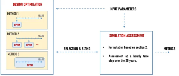
The main focus here is to have a common ground referential for the methods comparison. The process is described in figure3. With method 3, because the input parameters (i.e. load profiles, energy prices, equipment costs, etc.) and the modeling are the same in the design phase and in the assessment phase, the results from both cases (design and simulation) are obviously identical.
Figure 3: Assessment framework to compare the different methods. With method 3, because the input parameters (i.e. load profiles, energy prices, equipment costs, etc.) and the modeling are the same in the design phase and in the assessment phase, the results from both cases are identical.
Metrics:In addition to the total cost defined by (17), the net present value (NPV) is also computed to assess the
performance of each method as an output from the simulation phase. It is a standard metric to compare different investment projects [21,18] as it gives extra information about the profitability along the system lifetime. This lat-ter quantity is delat-termined by computing the difference between positive cash flows and investment costs. A positive NPV results in profit: the higher the NPV at the end of the horizon, the higher the profitability. In the study, cash flows correspond to savings compared to the baseline cost where all the electricity is purchased from the main upstream grid. In next section, design values, the NPV and computational times are going to be compared in order to have a fair comparison between those design methods. The best method is the one with the highest NPV while fulfilling the self-sufficiency constraint.
5. Numerical results
The aim of this section is to demonstrate novelties from the multi-time scale approach compared to the other resolution methods. Several examples will be introduced in order to highlight some specific points.
5.1. Case study
Input data and variables are listed below:
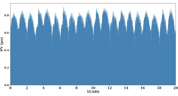
• The electrical demand and production profiles come from Ausgrid (australian distribution network) [22] which openly provides measured data at a 30 min time step from 300 residential consumers over 3 years. Among the available profiles, [23] identified a "clean dataset" which gathered 54 consumers around Sydney and Newcastle with similar power range. For each year of the 20-years horizon, 10 consumers profiles were randomly chosen and aggregated as input of the study (the solar profiles were also normalized). The demand and production variability between years is taken into account as each yearly profile is different from the others (see appendix
A).
• The tariff of electricity follows a peak/off-peak EDF "Tarif Bleu" [24]. For the sake of simplicity, no price evolution is taken into account over the 20 years.
Parameters 𝜂 − 𝜂+ 𝑒 𝑒 𝑝 𝑝 𝑛 𝑐 [0-1] [0-1] [0-1] [0-1] [h−1] [h−1] [-] Battery 0.8 0.8 0.2 0.8 1.5 1.5 2500 Table 2 Battery parameters
• The cost of storage system (Li-ion battery + converter) is given by [25] and decreases from 600 e/kWh in 2021 to 300 e/kWh in 2040 (see appendixA).
• The cost of solar panels including AC/DC converters is given by [26] and decreases from 1040 e/kWc in 2021 to 735 e/kWc in 2040 (see appendixA).
• The discount rate 𝜏 is set to 4.5%.
• Technical parameters for the battery are reported in table2.
The problem is modeled using Julia and JuMP package [27]. The IBM CPLEX 12.10 solver is then used to solve the problem. All the computations are run on a Intel Xeon(R) CPU E5-2697 v2 @ 2.70 GHz x 48 server.
5.2. Example 1: comparison with a self-sufficiency constraint set to 60%
With the current low electricity tariffs and costs of technologies, none of the three methods would invest in a Li-ion battery due to high capital expenditure compared to the expected savings on the operation. Thus, in order to compare the results from the different approaches, a first example is introduced where the self-sufficiency ratio is arbitrarily set to 60% in order to justify the installation of a storage system.
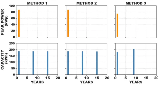
Figure4shows the planning strategy over the horizon for the three methods with a 60% self-sufficiency ratio. Note that the assets are assumed to be installed at the end of the first year in order to be operated the first hour of the second year. As shown in the figure, method 3 installs 75 kWp of solar panels and 182 kWh of battery the first year. Then, the battery is replaced once the 9th year by a new 205 kWh asset (+23 kWh compared to the initial investment) which occurs when the SoH reaches zero (see figure5). Figure5shows that the multi-time scale formulation handles correctly continuity issues and aging is controlled in order to install the new battery when the previous is out of order.
For the methods 1 and 2, the sizing results are the same in both cases with 88 kWp of PV and 188 kWh of storage installed the first year. Then the battery is replaced two times, the 8th and the 15th year with the same capacity as in the first year. Remind that method 2 reruns the optimization at the end of the battery lifetime whereas method 1 installs the same initial capacity at each replacement. The optimizer in method 2 does not take advantage of the investment cost reduction to increase the battery capacity when it has to be replaced. Indeed, even with cost decrease and current energy prices, it is not economically profitable to purchase battery storage so that the optimizer installs just enough battery and PV to ensure the self-sufficiency constraint fulfillment until the end of the simulated horizon. In both cases, the SoH is not controlled during operation and the battery need to be replaced one more time compared to method 3. However, at the end of the horizon, the storage systems are still "usable" and the remaining SoH (as a percentage of the total exchangeable energy) is 35% for both methods.
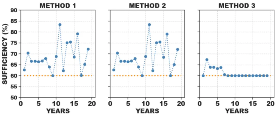
As shown in figure6, the self-sufficiency constraint is fulfilled each year with every method. Concerning method 3, the optimizer operates the DES and installs just enough capacity to fulfill the constraint each year with less margin than the other strategies. In contrast, method 1 and 2 optimize the system to fulfill the constraint during the worst years when the net energy demand is the higher which leads to greater self-sufficiency ratio for the rest of the years as the operation takes advantage of the system oversizing.
Economical results are depicted in table3. Note that with current economic hypothesis, the DES is not profitable over 20 years due to high installation cost of the battery. The reference cost is then lower than the optimal results obtained with the self-sufficiency constraint and the NPV is here given for information purpose only (negative values for all the methods). As shown in the table, the total discounted cost over the 20 years is 10% lower with method 3 than with the other methods. Note that the results of method 1 and 2 are approximately the same.
Finally, the better performances of method 3 are obtained at the cost of greater computational time with 24h long calculation where method 1 is run in only 5 min and method 2 in 15 min. Even if the number of variables and constraints
Figure 4: Planning strategy over the horizon with a 60% self-sufficiency ratio.
Figure 5: The battery SoH over the horizon with method 3 and a 60% self-sufficiency ratio. The SoH has been normalized by the maximum exchangeable energy in the figure.
are in the same range between the different methods (see table4), the complexity in the third approach is increased with the introduction of binary variables for the inter-year continuity on the investment decisions.
As a conclusion of this section, the results could be summed up as follows:
• With the multi-time scale approach, aging and number of replacement are controlled over the whole time horizon. • The sizing could whether be increased or down-scaled each year with method 3.
• It pays to control aging as the total discounted cost over the horizon is 10% lower than with the other strategies on the considered test case.
• The last method suffers from longer computational times compared to the other approaches.
5.3. Example 2: comparison with a higher electricity tariff
The aim of this section is to compare the three methods in a case where it is profitable to install a Li-ion battery without the self-sufficiency constraint. This could be obtained by assuming a lower investment cost of systems or with
Figure 6: Self-sufficiency constraint for each method after simulation. Its value was set to 60%.
Ref. Method 1 Method 2 Method 3 OPEX [ke] 185.8 62.5 62.5 72.4 CAPEX [ke] Li-ion - 205.4 205.2 167.9 PV - 87.0 87.0 74.8 Salvage [ke] - -8.4 -8.3 -Total [ke] 185.8 346.5 346.4 315.1 NPV [ke] - -160.7 -160.7 -129.3 CPU time - 5 min 3 × 5 min 24 h Table 3
Comparison of the total discounted costs over the 20 years and CPU time (computational time required to solve the model) between the three methods with a self-sufficiency ratio set to 60%. The reference case where all the electricity is bought from the grid and the NPV are given for information purpose.
Variables Constraints Method 1 & 2 876 022 1 927 304 Method 3 1 051 362 (38 bin) 2 444 637 Table 4
Comparison of the complexity between the three methods.
increased tariff of electricity. The latter strategy is chosen and the tariff of electricity is multiplied by 5 in order to have a battery installed the first year.
As shown in figure7, every method approximately installs the same battery capacity the first year (260 kWh). Then, both methods 2 and 3 take advantage of lower storage costs to increase the size of the battery. While method 3 only replaces the battery once with a 394 kWh asset (+134 kWh), method 2 replaces the storage twice with greater capacities: 280 kWh (+20kWh) the first time and 311 kWh (+51kWh) the second time. Similar to the test performed in the previous section, the battery is out of order at the end of the horizon for method 3 whereas it remains 50% and 54% of the total exchangeable energy for method 1 and 2 respectively. Concerning the PV, both method 1 and 2 install 116 kWp of solar panels which is 24 kWp greater than method 3. Compared to the previous section, the solar panel size increases when the electricity gets more costly, but no additional investment is made over the horizon. This latter aspect may be explained because when investment decisions are made, technologies are entirely replaced by new systems according to the modeling developed in this work. The cost induced is then proportional to new sizes instead
Figure 7: Planning strategy over the horizon with a tariff of electricity multiplied by 5.
Ref. Method 1 Method 2 Method 3 OPEX [ke] 929.0 210.5 197.6 213.0 CAPEX [ke] Li-ion - 280.3 296.8 270.8 PV - 115.8 115.8 91.8 Salvage [ke] - -16.6 -21.9 -Total [ke] 929.0 590.0 588.3 575.6 NPV [ke] - 339.1 340.8 353.4 CPU time - 5 min 3 × 5 min 24 h Table 5
Comparison of the total discounted costs over the 20 years and CPU time between the three methods with the tariff of electricity multiplied by 5.
of additional investment only. Thus, technologies with longer lifespan than the horizon are preferably installed the first year. Similar to previous section, the economic results are given in table5. As previously mentioned, the DES is profitable in every cases and the NPV at the end of the 20 years corresponds to profits compared to the baseline case without solar panels and battery. The differences between the NPV values are lower than in previous case: the profit is 4% greater with method 3 than method 1 and 3.6% greater than method 2. Note that the resulting NPV of method 1 and 2 are again approximately the same.
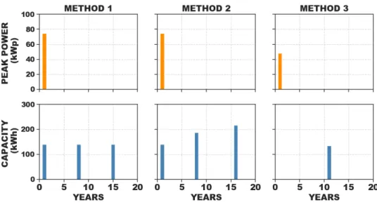
An interesting point is highlighted in figure8. In that case, the tariff of electricity is multiplied by 3. Unlike the other methods, method 3 installs 48 kWp of solar panels the first year but waits until the 11th year to purchase a 134 kWh battery when its cost is divided by 1.5. The multi-time scale approach not only optimizes the size of technologies, but also determines the optimal timing (investment pathway) to install the components along the horizon. This result is only made possible with the use of the proposed method 3 as the design is reconsidered each year in the formulation. This latter aspect gives more flexibility to the approach when strong evolution occurs over the input parameters.
Again, the NPV of method 1 and 2 are approximately the same while it is 20% higher for method 3 in this case.
5.4. Sensitivity analysis of the self-sufficiency ratio and electricity tariff over the design of the DES
The self-sufficiency ratio and electricity tariff consequences for the design of the DES are assessed by varying these latter parameters. The former quantity varies from 0% to 100% (100% when all the electricity consumed is provided byFigure 8: Planning strategy over the horizon with a tariff of electricity multiplied by 3. Unlike the other methods, method 3 waits until the 11th year to install the battery at a lower cost than first year.
Ref. Method 1 Method 2 Method 3 OPEX [ke] 557.4 233.7 214.3 345.7 CAPEX [ke] Li-ion - 153.2 179.8 35.3 PV - 74.2 74.2 48.1 Salvage [ke] - -6.2 -14.5 -Total [ke] 557.4 454.9 453.8 429.1 NPV [ke] - 102.4 103.5 128.4 Table 6
Comparison of the total discounted costs over the 20 years between the three methods with the tariff of electricity multiplied by 3.
the local generation) and the tariff of electricity is increasingly multiplied from 1 to 3. The multi-time scale approach is run for this section.
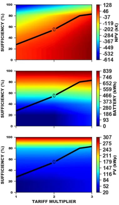
Figure9depicts the NPV as a function of both parameters. The black line delimits the area (under the line) where the DES is economically profitable over the 20 years (NPV greater or equal to zero). Remind that a NPV equals to zero means that the DES is paid back without any profits. With current electricity tariff and costs of technologies, no more than 30% of self-sufficiency is affordable without losing money over the 20 years. This is achieved with only 35 kWp of PV used in self-consumption without any battery to store the surplus of energy. When the tariff is multiplied by two and three, this value increases to 55% and 83% respectively.
Two specific cases are going to be further studied: 1) the self-sufficiency ratio is increased while the price of electricity remains fixed to its current value (tariff multiplier equals to 1); 2) the self-sufficiency constraint is set to zero and the tariff of electricity is increased up to 3 times the current price. The results are shown in figure9.
As we can observe in the first case, with 20% of self-sufficiency, only solar panels are installed while the battery remains too expensive. Then, the installed capacities increase exponentially with greater values of self-sufficiency. This is mostly due to the need for oversized assets in order to overcome extreme events where the production is low during long periods of time. As a result, with a 100% self-sufficiency constraint, the battery is mostly underused so that the maximum exchangeable energy is large enough to avoid any new costly replacement with the aging model developed in this work.
Figure 9: The net present value (top), the battery (middle) and the PV (bottom) cumulated capacities installed over the horizon as a function of the self-sufficiency and the tariff of electricity. The black isoline (NPV=0) delimits the area (under the line) where the DES is economically profitable over the 20 years (NPV greater or equal to zero).
In the second case, PV is installed even with current tariff and its size increases proportionally to the price of the electricity. In contrast, significant battery capacity is purchased over the horizon since the price has been multiplied by 3. In this case, the first investment is only made the 11th year as previously shown in section5.3.
The results of this section could be summed up as follows:
• With current electricity tariff, a maximum of 30% self-sufficiency is affordable without loosing money over the 20 years. This result is obtained by only installing 35 kWp of PV.
• With current electricity tariff, a battery is installed with the self-sufficiency constraint greater than 40%. Then, the size of systems grows rapidly, especially between 80% and 100% where the components are oversized to overcome extreme events where the production is low during long periods.
• Without the self-sufficiency constraint, a significant battery capacity is installed over the horizon since the tariff of electricity has been multiplied by 3.
6. Discussion and conclusions
A generic multi-time scale model for both the design and operation of energy systems was presented in this work. The integration of the aging and replacement dynamic into MILP formulation was depicted. Two examples were run to demonstrate novelties that could be extracted from this approach. Results were then compared to more standard approaches which consider a single equivalent year for the optimization of the design.
It is shown from the previous sections that it pays to control aging as the optimal solutions from the proposed multi-time scale model give the best economic results: the difference goes up to 20% of the total cost in some cases. This cost improvement is made possible because the multi-time scale model includes the interaction between design and operation with investment options at every year. Indeed, aging of the battery and thus, the number of replacements are controlled over the horizon, which is not possible with method 1 and 2. Moreover, method 3 gives more flexibility to the design of the DES as it can accommodate to input parameters evolution over time: the size of systems could be modified along the horizon by taking full advantage of the new information available. Furthermore, more than only optimizing the size of system, the multi-time scale approach also determines the investment strategy over the horizon. This latter point seems to be interesting for industrial who are willing to know when would be the best moment to invest in order to maximize profitability. Again, this feature could not be addressed by standard methods. Finally, even with the multi-time scale approach, a battery is installed over the horizon whether the self-sufficiency constraint is greater than 40% or the price of electricity is multiplied by 3.
Unlike [11] and [12], the multi-time scale formulation focuses on the interaction between the investment and the operation which is, to the best of the authors’ knowledge, rarely addressed in the literature. For the sake of simplic-ity, the equipment were assumed to be entirely replaced with the modeling developed in this work and no additional investment is made possible. This latter point is definitely a weakness of the model and future work need to be con-ducted in that direction to increase the value of the approach. Furthermore, the study was concon-ducted in a deterministic framework whereas the real problem is profoundly stochastic: investment and operation decisions have to be made without perfectly knowing the future. However, the aim of the study was to make a first evaluation in a deterministic framework to assess the cost reduction potential of the multi-time scale approach before going into more realistic mod-eling with uncertainties. In order to include the stochastic nature of the problem and apply the methodology to more complex energy systems, computational times need to be reduced and further resolution methods have to be explored (the better performances of method 3 are obtained at the cost of greater computational time with 24h long calculation where method 1 is run in only 5 min and method 2 in 15 min). For instance, the decomposition methods developed by [15] seems to be a great candidate to address this challenge.
Despite these aforementioned limitations, it seems that the multi-time scale approach could be a promising direction in order to improve the income of a given project when energy rates are low and standard strategies fail to find out a profitable design. The model has proven to be a relevant approach and this work could be seen as a starting point for whoever would be interested in the integration of the interaction between investment and operation in more general energy models and complex analysis.
7. Acknowledgments
This work has been supported by the ADEME (french national agency on environment, energy and sustainable development) in the framework of the HYMAZONIE project.
References
[1] D. Connolly, H. Lund, B. V. Mathiesen, and M. Leahy. A review of computer tools for analysing the integration of renewable energy into various energy systems. Applied Energy, 87(4):1059–1082, April 2010.
[2] Paolo Gabrielli, Matteo Gazzani, Emanuele Martelli, and Marco Mazzotti. Optimal design of multi-energy systems with seasonal storage.
Applied Energy, 219:408–424, June 2018.
[3] Georgios Mavromatidis, Kristina Orehounig, and Jan Carmeliet. Uncertainty and global sensitivity analysis for the optimal design of distributed energy systems. Applied Energy, 214:219–238, March 2018.
[4] Benjamin Guinot, Bénédicte Champel, Florent Montignac, Elisabeth Lemaire, Didier Vannucci, Sebastien Sailler, and Yann Bultel. Techno-economic study of a PV-hydrogen-battery hybrid system for off-grid power supply: Impact of performances’ ageing on optimal system sizing and competitiveness. International Journal of Hydrogen Energy, 40(1):623–632, January 2015.
[5] Remy Rigo-Mariani, Bruno Sareni, and Xavier Roboam. Integrated Optimal Design of a Smart Microgrid With Storage. IEEE Transactions
on Smart Grid, 8(4):1762–1770, July 2017.
[6] Rémy Rigo-Mariani, Sean Ooi Chea Wae, Stefano Mazzoni, and Alessandro Romagnoli. Comparison of optimization frameworks for the design of a multi-energy microgrid. Applied Energy, 257(113982), January 2020.
[7] Yun Yang, Shijie Zhang, and Yunhan Xiao. An MILP (mixed integer linear programming) model for optimal design of district-scale distributed energy resource systems. Energy, 90:1901–1915, October 2015.
[8] Mohammad Ameri and Zahed Besharati. Optimal design and operation of district heating and cooling networks with CCHP systems in a residential complex. Energy and Buildings, 110:135–148, January 2016.
[9] Stefano Bracco, Gabriele Dentici, and Silvia Siri. DESOD: a mathematical programming tool to optimally design a distributed energy system.
Energy, 100:298–309, April 2016.
[10] Nikolaos E. Koltsaklis and Athanasios S. Dagoumas. State-of-the-art generation expansion planning: A review. Applied Energy, 230:563–589, November 2018.
[11] Yixian Liu, Ramteen Sioshansi, and Antonio J. Conejo. Multistage Stochastic Investment Planning With Multiscale Representation of Uncer-tainties and Decisions. IEEE Transactions on Power Systems, 33(1):781–791, January 2018.
[12] Emilio L. Cano, Markus Groissböck, Javier M. Moguerza, and Michael Stadler. A strategic optimization model for energy systems planning.
Energy and Buildings, 81:416–423, October 2014.
[13] Pierre Haessig, Hamid Ben Ahmed, and Bernard Multon. Energy storage control with aging limitation. In 2015 IEEE Eindhoven PowerTech, pages 1–6, Eindhoven, Netherlands, June 2015. IEEE.
[14] Roman Le Goff Latimier. Gestion et dimensionnement d’une flotte de véhicules électriques associée à une centrale photovoltaïque:
co-optimisation stochastique et distribuée. PhD thesis, Université Paris-Saclay, ENS Cachan, 2016.
[15] Pierre Carpentier, Jean-Philippe Chancelier, Michel De Lara, and Tristan Rigaut. Algorithms for two-time scales stochastic optimization with applications to long term management of energy storage. hal-02013969, 2019.
[16] Yang Li, Mahinda Vilathgamuwa, San Shing Choi, Troy W. Farrell, Ngoc Tham Tran, and Joseph Teague. Development of a degradation-conscious physics-based lithium-ion battery model for use in power system planning studies. Applied Energy, 248:512–525, August 2019. [17] Sylvain Quoilin, Konstantinos Kavvadias, Arnaud Mercier, Irene Pappone, and Andreas Zucker. Quantifying self-consumption linked to solar
home battery systems: Statistical analysis and economic assessment. Applied Energy, 182:58–67, November 2016.
[18] Tom Lambert, Paul Gilman, and Peter Lilienthal. Micropower System Modeling with Homer. In Felix A. Farret and M. Godoy Simões, editors, Integration of Alternative Sources of Energy, pages 379–418. John Wiley & Sons, Inc., Hoboken, NJ, USA, April 2006.
[19] R. Luna-Rubio, M. Trejo-Perea, D. Vargas-Vázquez, and G. J. Ríos-Moreno. Optimal sizing of renewable hybrids energy systems: A review of methodologies. Solar Energy, 86(4):1077–1088, April 2012.
[20] Bei Li, Robin Roche, Damien Paire, and Abdellatif Miraoui. Sizing of a stand-alone microgrid considering electric power, cooling/heating, hydrogen loads and hydrogen storage degradation. Applied Energy, 205:1244–1259, November 2017.
[21] A. Hina Fathima and K. Palanisamy. Optimization in microgrids with hybrid energy systems – A review. Renewable and Sustainable Energy
Reviews, 45:431–446, May 2015.
[22] Ausgrid. Solar home electricity data - Ausgrid, 2020.
[23] Elizabeth L. Ratnam, Steven R. Weller, Christopher M. Kellett, and Alan T. Murray. Residential load and rooftop PV generation: an Australian distribution network dataset. International Journal of Sustainable Energy, 36(8):787–806, September 2017.
[24] EDF. Electricité - Tarif Bleu EDF : Option Base ou Heures Creuses, 2020.
[25] N Lebedeva, D Tarvydas, and I Tsiropoulos. Li-ion batteries for mobility and stationary storage applications: scenarios for costs and market growth. Technical report, European commission, Joint Research Center, 2018. OCLC: 1111111915.
[26] IRENA. Renewable power generation costs in 2018. Technical report, International Renewable Energy Agency, Abu Dhabi, 2019. [27] Iain Dunning, Joey Huchette, and Miles Lubin. JuMP: A Modeling Language for Mathematical Optimization. SIAM Review, 59(2):295–320,
A. Appendix
Figure 10: Time-series of energy demand over the 20 years.
Figure 12: Duration curves for the energy demand (left) and PV production (right) for each year. The mean value is depicted in blue in the figure. The orange area corresponds to the min/max envelope over the 20 years.