Research Article
Edgars Jakobsons*
Scenario aggregation method for portfolio
expectile optimization
DOI: 10.1515/strm-2016-0008
Received April 21, 2016; accepted August 19, 2016
Abstract: The statistical functional expectile has recently attracted the attention of researchers in the area of risk management, because it is the only risk measure that is both coherent and elicitable. In this article, we consider the portfolio optimization problem with an expectile objective. Portfolio optimization prob-lems corresponding to other risk measures are often solved by formulating a linear program (LP) that is based on a sample of asset returns. We derive three different LP formulations for the portfolio expectile optimization problem, which can be considered as counterparts to the LP formulations for the Conditional Value-at-Risk (CVaR) objective in the works of Rockafellar and Uryasev [43], Ogryczak and Śliwiński [41] and Espinoza and Moreno [21]. When the LPs are based on a simulated sample of the true (assumed continuous) asset returns distribution, the portfolios obtained from the LPs are only approximately optimal. We conduct a numerical case study estimating the suboptimality of the approximate portfolios depending on the sample size, number of assets, and tail-heaviness of the asset returns distribution. Further, the computation times using the three LP formulations are analyzed, showing that the formulation that is based on a scenario aggregation approach is considerably faster than the two alternatives.
Keywords: Expectile, portfolio optimization, linear programming, scenario aggregation MSC2010: 90C05, 91G10, 62E17
1 Introduction
The expectile is introduced in [40] as the minimizer of the expectation of an asymmetric quadratic scoring function with respect to a point forecast e∈ ℝ of a random variable L,
eτ(L) = argmin
e∈ℝ E[(τ𝟙{L>e}+ (1 − τ)𝟙{L<e})(L − e)
2].
(1.1) Until recently, it was known almost exclusively amongst statisticians and was applied in regression analysis; see, e.g., [19, 20, 45]. Currently, the expectile is making a debut in the area of risk management, due to func-tional properties that make it suitable as a risk measure for regulatory and portfolio management purposes. The axioms of coherence, introduced in the seminal paper of Artzner, Delbaen, Eber and Heath [4], are often considered as indispensable for any risk measure used in practice, as motivated by their interpretation, as well as the resultant mathematical tractability. However, the most commonly used risk measure, Value-at-Risk (VaR) [28], is not coherent. In particular, VaR does not satisfy the axiom of subadditivity, which requires that the risk measure captures diversification. Recently, Gneiting [23] brought another property, elicitability to the foreground. A risk measure is said to be elicitable if it is a minimizer of the expectation of some scoring function, which depends on the point forecast and the true observed loss. Gneiting [23] further showed that the well-known coherent risk measure Expected Shortfall (ES, also known as the Conditional Value-at-Risk, CVaR) is not elicitable. Some authors associate elicitability with being able to back-test risk models based on
*Corresponding author: Edgars Jakobsons: RiskLab, Department of Mathematics, ETH Zurich, 8092 Zurich, Switzerland, e-mail: [email protected]
the quality of forecasts that have been made in the past, a crucial requirement from a regulatory perspective [14, 15, 25]. Other authors argue that elicitability is relevant for relative comparisons between estimators, but not for absolute significance testing [2].
In [7, 18, 46], it is shown that the only risk measure that is both elicitable and coherent is the expectile (for τ∈ [1/2, 1), when positive outcomes for the random variable (rv) L represent losses). This makes the expectile an interesting object for research with the aim of assessing its suitability for measuring risk in practice. First such studies include [7, 9, 27, 32].
Another property of the expectile can be observed from the first order conditions on the optimization in (1.1), namely, eτ(L) is the unique solution of
(1 − τ)E[(eτ− L)𝟙{L<eτ}] = τE[(L − eτ)𝟙{L>eτ}].
In particular, while VaR an ES focus only on extreme losses, the expectile balances gains and losses, which is desirable for portfolio management. Because of this, the expectile is also closely related to the Omega performance measure of Keating and Shadwick [30]; see [42, p. 128]. Bellini and Di Bernardino [9] also point out the expectile has an intuitive interpretation in terms of its acceptance set, namely, a risk is acceptable (for a regulator) if its gains-loss ratio [11] is sufficiently high. See [9] and references therein for further properties of the expectile risk measure.
Before we conclude this section, we provide a simple iterative procedure for computing the expectile of a discrete rv, based on the method in [20] for fitting a linear regression with asymmetric least squares mini-mization. A special case of this method yields a procedure for computing the expectile of a discrete rv L such that P(L = ℓi) = pi, i∈ {1, . . . , n}. Starting from a trial value b0∈ ℝ, we update iteratively for k = 0, 1, 2, . . .:
bk+1= n ∑ i=1 w(k)i ℓi( n ∑ i=1 w(k)i ) −1 , where w(k)i = |τ − 𝟙{ℓi>bk}|pi. (IRLS)
This is the method of iteratively reweighted least squares (IRLS).¹ The sequence converges to the corresponding expectile, i.e., limk→∞bk= eτ(L). In practice, this procedure typically converges within a few iterations.
The rest of this article is organized as follows. In Section 2, we introduce the portfolio optimization prob-lem with an expectile objective and derive three different LP formulations for this probprob-lem, when the asset returns follow a finite discrete distribution. In Section 3, we analyze the quality of the portfolios obtained from the LPs, when the latter are based on a Monte Carlo sample from the true (assumed continuous) asset returns distribution. We also compare the computation times required for solving each of the three LP formulations. Finally, Section 4 concludes.
2 Portfolio optimization
We consider a standard single period portfolio optimization problem, where a given amount w> 0 of wealth is to be invested in d available assets. If the current value of an asset is Sj(0) > 0 and its value at the end of the
period (investment horizon) is Sj(1) ∈ L1(Ω, A, P), then the return of this asset is given by Yj= Sj(1)/Sj(0) − 1, j = 1, . . . , d. Denoting by Y = (Y1, . . . , Yd)⊤the vector of asset returns and by x∈ ℝdthe vector of monetary amounts invested in the corresponding assets at the beginning of the period, the random variable L= −x⊤Y corresponds to the portfolio loss. The possible portfolio positions (values of x) have to satisfy a budget con-straint x⊤1 ⩽ w and typically further constraints, such as the expected returns constraint x⊤μ ⩾ R (where μ = E[Y] and R ∈ ℝ), no-short-sales constraint x ⩾ 0 or diversification constraints b ⩽ x ⩽ b for b, b ∈ ℝd.² We denote the set of feasible portfolios by X, and remark that it is often polygonal. The corresponding
1 The analogous procedure for continuous distributions is provided in [27]; in fact, it is Newton’s method applied to the opti-mization problem (1.1).
2 The inequalities for vectors are to be understood component-wise. The notation 1 = (1, . . . , 1)⊤∈ ℝd is used.
portfolio optimization problem with the expectile risk measure as the objective is minimize eτ(−x⊤Y) over x ∈ ℝd
subject to x ∈ X.
This is a d-dimensional optimization problem, where the expectile objective is only implicitly defined in (1.1). Furthermore, the definition involves expectations of the portfolio loss over events of the form{−x⊤Y > e}. In general, such an expectation corresponds to a d-dimensional integral and is numerically cumbersome to evaluate. However, in special cases, the problem can be simplified, for example, when the asset returns vector follows a multivariate elliptical distribution.
Elliptical distributions Y∼ Ed(μ, Σ, ψ) are defined by the corresponding characteristic function φY(t) = exp(it⊤μ)ψ(1
2t ⊤
Σ t), t ∈ ℝd.
The elliptical family has the property that any linear combination x⊤Y of the margins (assets) with weights x ∈ ℝdbelongs to a particular location-scale family (determined by ψ), with parameters μ⊤x and √x⊤Σ x respectively; see also [39, Section 3.3]. We have
x⊤Y= μd ⊤x + Z√x⊤Σ x, where Z∼ E
1(0, 1, ψ). (2.1)
Furthermore, since the expectile is a coherent risk measure for τ∈ [1/2, 1) (see [46]), it satisfies the axioms of monotonicity, subadditivity, translation invariance and positive homogeneity. The latter two are stated as follows:
∙ translation invariance: for c∈ ℝ, eτ(c + L) = c + eτ(L),
∙ positive homogeneity: for s⩾ 0, eτ(sL) = seτ(L).
Applying these properties in (2.1) and using Z= −Z, we obtaind
eτ(−x⊤Y) = −μ⊤x + λτ√x⊤Σ x, where λτ = eτ(Z). (2.2) Thus, under an expected returns constraint μ⊤x = R, the expectile optimization problem is solved by the minimal variance portfolio of [38]. See also [39, Proposition 6.13], where this result is stated in full generality, for all law-determined risk measures that are positive homogeneous and translation invariant. This useful property will enable using the multivariate Student-t distribution (which is elliptical) as a benchmark for the numerical case study in Section 3.
In general, for multivariate distributions that do not have such symmetry properties, the portfolio problem cannot be solved analytically. Examples of particular relevance for modeling skewed asset returns distributions can be found in the class of normal mean-variance mixtures. A prime example is the class of generalized hyperbolic distributions [5], as well as subclasses of it, such as the NIG [6], VG [33] and the skew-t distribution [1].
However, it is easy to obtain large Monte Carlo (MC) samples from these multivariate mixture distri-butions. In the case of a discrete asset returns distribution (e.g., based on the MC sample or the empirical distribution of historical returns), the portfolio optimization problems with risk objectives such as the mean absolute deviation [31], CVaR [43], and the Omega ratio [29] can be formulated as Linear Programs (LP). These results are of considerable practical importance, since LP formulations are solvable for a large number of assets and constraints, and have been a crucial tool for portfolio selection since the advent of computers; see [3, 44] for early examples and [34–37] for a recent overview.
In the following sections, we derive three LP formulations for the portfolio optimization problem with an expectile objective. In Section 2.1, the primal formulation is derived, in Section 2.2, the dual formulation, and in Section 2.3, a scenario aggregation approach is presented.
2.1 Primal LP formulation
The definition of the expectile in (1.1) is useful for fitting regression models in statistical analysis. For the portfolio optimization problem, however, using this definition would lead to a nested optimization problem,
which are known to be computationally costly. A so-called dual representation of the expectile that is more suitable for our purpose is provided in [17] in terms of a set of generalized scenarios (probability measures Q≪ P); see also [16, p. 36]. This representation stated in terms of the corresponding Radon–Nikodym deriva-tives φ= dQ/dP is as follows. For L ∈ L1(Ω, A, P) and τ ∈ [1/2, 1),
eτ(L) = sup φ∈Mτ
E[Lφ], (2.3)
where
Mτ= {φ ∈ L∞(Ω, A, P) : φ ⩾ 0, E[φ] = 1, there exists an m > 0 such that (1 − τ)m ⩽ φ ⩽ τm}. (2.4) In fact, a risk measure is coherent if and only if it admits a representation of this type, called robust represen-tation; see [22, Proposition 4.14].
When the probability space is finite and discrete, Ω= {ω1, . . . , ωn}, the representation in (2.3) can be
formulated as an LP. In particular, we define the following optimization problem for computing eτ(L), where L is a discrete rv such that P(L = ℓi) = P(ωi) = pi, i∈ {1, . . . , n}. Recall that we assume τ ∈ [1/2, 1). Then
maximize n ∑ i=1 ℓipiφi over m∈ ℝ, φ ∈ ℝn (D1) subject to n ∑ i=1 piφi= 1, (1 − τ)m ⩽ φi⩽ τm, m ⩾ 0, φi⩾ 0, i = 1, . . . , n.
The decision variables φirepresent the Radon–Nikodym derivative evaluated at outcome ωi. Taking the dual of the problem (D1) yields
minimize ζ over ζ ∈ ℝ, u, v ∈ ℝn (P1) subject to piζ − ui+ vi⩾ piℓi, ui⩾ 0, vi⩾ 0, i = 1, . . . , n, (1 − τ) n ∑ i=1 ui− τ n ∑ i=1 vi⩾ 0.
Notice that in this formulation, the loss valuesℓiare separated from the decision variables. This allows us to express the losses in terms of the portfolio weights, and formulate a joint optimization problem that is still linear, as follows. In the portfolio problem, the random variable L represents portfolio losses, L= −x⊤Y, where x∈ ℝd is the vector of portfolio weights and Y is a d-dimensional random vector of asset returns. Suppose that the set of admissible portfolio weights is given by X⊂ ℝd, which is a polytope generated by some linear constraints. We also assume that Y follows a discrete distribution, with P(Y = yi) = pi, i∈ {1, . . . , n}. Substitutingℓi= −x⊤yiinto the problem (P1) yields the primal LP formulation of the portfolio optimization problem.
minimize ζ over x∈ ℝd, ζ ∈ ℝ, u, v ∈ ℝn (Primal)
subject to pix⊤yi+ piζ − ui+ vi⩾ 0, ui⩾ 0, vi⩾ 0, i = 1, . . . , n, x ∈ X, (1 − τ) n ∑ i=1 ui− τ n ∑ i=1 vi⩾ 0.
This is an LP with d+ 1 + 2n decision variables and n + 1 joint inequality constraints (apart from those imposed by X). This formulation can be considered as the expectile counterpart of the LP formulation for the CVaR objective in [43]. For the CVaR problem, the corresponding LP has only d+ 1 + n decision variables, because the corresponding set of generalized scenarios has a simpler structure; see [22, Theorem 4.47].
In [8], a similar LP formulation to (Primal) for the expectile problem was derived, using the following set of Radon–Nikodym derivatives from [10], which is mathematically equivalent to (2.4):
Mτ = {φ ∈ L∞(Ω, A, P) : φ > 0, E[φ] = 1, ess sup(φ)
ess inf(φ) ⩽
τ
1− τ}. The latter inequality constraints were formalized in the discrete case as n(n − 1) constraints
With this formulation, solving the corresponding LPs within a reasonable computation time is possible only up to n= 1000, because this already yields more than 999,000 decision variables in the primal formulation of the portfolio optimization problem. In our (Primal) formulation, the number of decision variables grows linearly in n, because in (D1) there are only 2n constraints on φ, at the expense of only one additional decision variable m. This allows solving LPs that are based on much larger sample sizes; see Section 3.
2.2 Dual LP formulation
It was demonstrated in [41] that the portfolio optimization problem with the CVaR objective can be solved considerably faster by using the dual formulation instead of the primal one. Since the expectile portfolio optimization problem has a similar structure, we also formulate the dual LP to (Primal). In Section 3.2, the computation times using the different formulations will be analyzed to determine which formulation is com-putationally the most efficient.
To state the dual problem explicitly, we specify the set of admissible portfolios as X = {x ∈ ℝd
: 1⊤x = 1, xk⩾ 0, k = 1, . . . , d}, (2.5)
which corresponds to a fully invested portfolio with wealth normalized to 1 (without loss of generality, since coherent risk measures are positively homogeneous), and under the no-short-sales constraint. Note that further linear constraints can be added, which would then correspond to additional decision variables in the dual problem.
The dual problem to (Primal) for portfolio expectile optimization is the following:
maximize η over η, m∈ ℝ, φ ∈ ℝn (Dual)
subject to n ∑ i=1 piφi= 1, (1 − τ)m ⩽ φi⩽ τm, m ⩾ 0, φi⩾ 0, i = 1, . . . , n, n ∑ i=1 piy(k)i φi+ η ⩽ 0, k = 1, . . . , d,
where y(k)i denotes the return of asset k= 1, . . . , d in outcome i = 1, . . . , n. The optimized objective value
η∗
is the expectile eτ(−x∗⊤Y) for the optimal portfolio x∗. The optimal portfolio weights are given by the Lagrange multipliers corresponding to the last d inequality constraints.
2.3 Aggregation algorithm
Recently, Espinoza and Moreno [21] proposed an iterative solution procedure for the portfolio CVaR optimiza-tion problem, based on (dis-)aggregaoptimiza-tion of scenarios.³ In [26], this method was found be the advantageous in terms of computation time, in particular, for a large sample size n and a high probability level α of the CVaRα
objective. In this subsection, we formulate the Aggregation algorithm for the portfolio expectile optimization problem.
The idea is based on the property that, for the optimal solution of (Dual), the Radon–Nikodym derivative takes values in the range φi∈ [(1 − τ)m, τm], i = 1, . . . , n, with most outcomes φiat the endpoints of this interval. In fact, from Proposition 8 in [10] follows that an optimal solution of (D1) is given by
φi= (1 − τ)m𝟙{ℓi⩽ eτ} + τm𝟙{ℓi> eτ}, i = 1, . . . , n, m = 1
(1 − τ) P(L ⩽ eτ) + τ P(L > eτ), (2.6)
where eτ= eτ(L). Further, if a solution has decision variables φi∈ ((1 − τ)m, τm) that lie strictly inside the
interval, they correspond to lossesℓi= eτ. This leads to the idea of reducing the number of decision variables
by representing the values of φiover several outcomes with a single variable; this does not affect the opti-mality, as long as these outcomes correspond to losses that are all either above or below the level eτ. This approach is called scenario aggregation.
This method is implemented by partitioning the set of all outcomes and constraining the values φito be constant within each set of this partition. Specifically, for a partition N= {N1, . . . , Nñ} of the set of indices
{1, . . . , n} into ̃n subsets, we add constraints φi= φjwhenever i, j∈ Nkfor some k= 1, . . . , ̃n. This problem can be represented using fewer decision variables, as follows.
maximize η over η, m∈ ℝ, ̃φ ∈ ℝñ (Aggregated)
subject to ̃ n ∑ i=1 ̃piφ̃i= 1, (1 − τ)m ⩽ ̃φi⩽ τm, m ⩾ 0, ̃φi⩾ 0, i = 1, . . . , ̃n, ̃ n ∑ i=1 c(k)i φ̃i+ η ⩽ 0, k = 1, . . . , d, where ̃pi= ∑ j∈Ni pj and ci= ∑ j∈Ni pjyj, i = 1, . . . , ̃n.
Let ̃x be the vector of portfolio weights given by the Lagrange multipliers corresponding to the last d inequality constraints in the problem (Aggregated). This portfolio may not be optimal for the original problem, because we have implicitly imposed additional constraints on (Dual). The expectile for the loss of this portfolio can be computed, e.g., by solving (P1) or (D1) withℓi= − ̃x⊤yi. However, we recommend using (IRLS) for this purpose, as it is considerably faster.
Denote the optimal objective value of the constrained problem (Aggregated) by eNτ, the optimal value of
the original problem (Dual) by eOPTτ , and the expectile (as computed using (IRLS)) of the approximate portfolio
̃x by ex̃
τ. Then the following inequalities hold:
eNτ ⩽ eOPT
τ ⩽ exτ̃. (2.7)
The first inequality holds because (Aggregated) is equivalent to a more constrained version of the maximiza-tion problem (Dual); the second – because the portfolio ̃x is feasible for the portfolio optimization problem (Primal) when X is given by (2.5). Hence, solving the (Aggregated) problem yields an interval for the true optimal portfolio expectile.
The value exτ̃also induces a partitioning{M1, M2, M3} of the scenario indices i ∈ {1, . . . , n},
M1= {i : − ̃x⊤yi< exτ̃}, M2= {i : − ̃x⊤yi= exτ̃}, M2= {i : − ̃x⊤yi> exτ̃}.
This partitioning can then be used to refine our previous partitioning N by splitting the sets that contain both “good” and “bad” scenarios, namely,ℓithat are below, respectively, above the expectile level of the current portfolio. These ideas are combined in the following scenario aggregation algorithm for portfolio expectile optimization.
Aggregation algorithm Require: Stopping gap δ ⩾ 0 1. InitiateN ← {{1, . . . , n}} 2.loop
3. Solve (Aggregated), obtain eNτ and ̃x. 4. Compute ex̃
τ = eτ(− ̃x⊤Y) using (IRLS) and construct M1, M2, M3.
5.if ex̃ τ− eNτ ⩽ δ then 6.return Solution( ̃x) 7.else 8. LetN ← {N ∩ Mj: N ∈N, j ∈ {1, 2, 3}}. end
At the first iteration of the Aggregation algorithm, the (IRLS) procedure in Step 4 can be initialized at
b0= E[− ̃x⊤Y], and in subsequent iterations the expectile of the previous portfolio can be used as the starting value for (IRLS). Note that the Aggregation algorithm will need to solve several instances of (Aggregated). However, because of the scenario aggregation, these instances will be of a considerably smaller size than (Dual), which may lead to savings in the total computation time. The computation times are analyzed in Section 3.2.
Lemma 1. The Aggregation algorithm with δ = 0 returns a solution after a finite number of iterations.
Proof. The proof is parallel to that of [21, Lemma 1]. We only need to show that in each iteration the
number of sets in the partition N strictly increases; the number of iterations is then bounded by the number of scenarios n. To this end, we define a Lagrangian relaxation of (Aggregated) by penalizing the violation of the last d inequality constraints by ξ∈ ℝd+:
L(ξ) = maximize η + ξ⊤ (− ̃ n ∑ i=1 ciφ̃i− η) over η, m ∈ ℝ, ̃φ ∈ ℝñ subject to ̃ n ∑ i=1 ̃piφ̃i= 1, (1 − τ)m ⩽ ̃φi⩽ τm, m ⩾ 0, ̃φi⩾ 0, i = 1, . . . , ̃n.
Suppose that in Step 8 of the Aggregation algorithm, the number of sets in the partition does not increase, i.e. N is already a refinement of{M1, M2, M3}. Then, since exτ̃ is the optimal objective value of (D1) with
ℓi= − ̃x⊤yi, by (2.6) there exists a solution(m∗, φ∗) of (D1) such that φ∗ is constant on each of the sets
M1, M2, M3. Hence, this solution is also constant on the sets in partition N= {N1, . . . , Nñ}, so we can define
̃
φ∗
i = φ∗j using any j∈ Nifor i= 1, . . . , ̃n. Then, (η, m∗, ̃φ
∗
) is feasible for L for any η ∈ ℝ. With these feasible values, setting ξ= ̃x, the objective of L is equal to exτ̃, so exτ̃ ⩽ L( ̃x). Further, since ̃x is the optimal Lagrange
multiplier from (Aggregated) corresponding to the relaxed constraints, we obtain L( ̃x) = eNτ . Combining
with (2.7), it follows that exτ̃= eNτ, which completes the proof.
Remark 1. The formulations (Dual), (Aggregated), and hence the Aggregation algorithm can be adapted to accommodate further portfolio constraints of the form Ax= b beyond the definition of X in (2.5). If b ∈ ℝq, we replace the decision variable η by vector η∈ ℝq, the objective by b⊤η, and put (A⊤η)(k)in the constraints instead of η.
3 Numerical case study
In this section, we analyze the LP problem of expectile portfolio optimization from two perspectives. First, note that typically it is assumed that the true asset returns distribution is continuous, therefore the LP formulations are based on a discrete approximation of the true distribution. As a consequence, the obtained portfolios may be suboptimal. In Section 3.1, we analyze the suboptimality of the portfolios given by LP approximations, based on the sample size and other factors. Second, to determine the best approach for solving the LPs, we also compare the computation times using the formulations (Primal), (Dual), and the Aggregation algorithm; see Section 3.2.
Setting μ= 0 in (2.1), we note that for elliptical asset returns distributions, the portfolio expectile opti-mization problem is solved by the minimum variance portfolio, namely,
x∗= argmin
x∈ℝd
x⊤Σ x subject to x∈ X. (QP)
This is a quadratic programming problem with linear constraints and only d decision variables, which can be solved efficiently using standard optimization software. Further, note that this yields the true optimal port-folio for the corresponding elliptical asset returns distribution, without relying on discrete approximations. Therefore, these distributions can be used as benchmark for evaluating the quality of approximate solutions obtained from the LPs. In this case study, we will consider d-variate normal Nd(0, Σ) and Student td(0, Σ, ν)
distributions for asset returns. The parameters are selected as follows. The location vector is set to zero, because this enables obtaining the benchmark portfolio using (QP), furthermore, for asset returns data the means are indeed typically close to zero. To obtain a realistic dependence structure, for the scale matrix Σ we use the covariance matrix of financial time series. In particular, the covariance matrix is computed using the daily returns of up to d= 101 constituents of the FTSE 100 index from 2-Jan-2003 to 18-Sep-2014 (the same dataset as used in [26]). Since Σ is only the scale, not the covariance matrix for Student-t, it is not intended that these parameters are a good fit for the original data, only a reasonable choice for a case study. Blattberg and Gonedes [13] estimate the degrees of freedom parameter for most stock daily returns to be in the range
ν ∈ (4, 5), with occasional values above and below. Hence, in our case study we consider a representative set
of values ν∈ {3, 5, 10, ∞}. Note that the limiting case ν = ∞ is the normal distribution. The optimization is performed over fully invested portfolios under the no-short-sales constraint, as defined in (2.5).
From (2.2) it follows that the portfolio loss expectile for any portfolio x∈ X in this case study can be computed using the formula
eτ(−x⊤Y) = λτ√x⊤Σ x, where λτ = eτ(Z), Z ∼ t1(0, 1, ν). (3.1) We will consider expectile levels τ∈ {0.99, 0.999, 0.9999}. In Table 1, the values of λτ are listed for the considered values of τ and Student-t parameters ν.
ν
τ ∞ 10 5 3
0.99 1.72 2.03 2.50 3.63 0.999 2.44 3.15 4.43 8.12 0.9999 3.06 4.42 7.31 17.63
Table 1. Expectile eτ(L) at levels τ ∈ {0.99, 0.999, 0.9999} for a (standard) Student-t distributed rv L with ν ∈ {∞, 10, 5, 3} degrees of freedom.
Since the expectile is currently not being used as a regulatory risk measure, it is not clear what values of τ would be considered reasonable. To give an intuition for how far in the tail of the loss distribution the expec-tile levels τ∈ {0.99, 0.999, 0.9999} are, we compare them to the levels of other well-known risk measures. Table 2 lists the corresponding probability levels α and β that would yield the same value for VaRα(L) and
ESβ(L) as that of eτ(L). Note that a Student-t distribution with ν = ∞ is the normal distribution; and in this
case the corresponding probabilities are, e.g., 95.7 %, 99.3 %, 99.9 % for VaR. These are close to the levels typically considered for VaR. The comparison in the case of the normal distribution is relevant, since appar-ently, a similar approach was taken by the Basel Committee on Banking Supervision [47], when moving from VaR0.99as the risk measure for the trading book capital requirements to ES0.975. Adjusting the probability level β, so that the numerical value of ESβ(L) for a normally distributed rv L matches VaR0.99(L) = 2.3263, yields β≈ 0.97423, which is rounded to β = 0.975 (adjusting τ so that eτ(L) matches VaR0.99(L) would yield τ≈ 0.99855).
α such that VaRα(L) = eτ(L) β such that ESβ(L) = eτ(L)
ν ν
τ ∞ 10 5 3 ∞ 10 5 3
99 95.71 96.50 97.29 98.19 89.18 90.62 92.14 94.09 99.9 99.26 99.49 99.66 99.80 98.08 98.58 98.98 99.35 99.99 99.89 99.94 99.96 99.98 99.71 99.82 99.89 99.93
Table 2. Probability levels α and β such that VaRα(L), respectively, ESβ(L) is equal to the expectile at level τ ∈ {0.99, 0.999, 0.9999} of a Student-t distributed rv L with ν ∈ {∞, 10, 5, 3} degrees of freedom. The
3.1 Suboptimality
When a continuous asset returns distribution is approximated by a discrete one, and a portfolio is selected by solving an LP based on the discrete approximation, the selected portfolio may not be optimal for the original asset returns distribution. To estimate the suboptimality of the portfolios that are obtained using such LP approximations, we conducted a large number of experiments, changing the number of assets
d ∈ {3, 5, 10, 25, 50, 101} and Student-t parameter ν ∈ {3, 5, 10, ∞}, in each case generating 100 MC
sam-ples of size n, 103⩽ n ⩽ 106, and solving the corresponding instances of LPs for τ∈ {0.99, 0.999, 0.9999}. Let Y∼ td(0, Σ, ν) be a rv with the true asset returns distribution and let ̃Y ∼ UNIF{y1, . . . , yn} be the
discrete approximation based on an MC sample. Further, denote by xLPthe portfolio obtained by solving the LP approximation, and by xQPthe true optimal portfolio, given by (QP). We first point out that, to estimate the suboptimality, one cannot use the objective value of the LP, eτ(−x⊤LPY) (the perceived expectile), because it is̃
a biased estimate of the true expectile of this portfolio, eτ(−x⊤LPY). The latter can be computed using (3.1),
and so can the true optimal expectile eτ(−x⊤QPY). Hence, we can separate the error into two parts, bias and
suboptimality, computed relative to the true optimum as subopt= eτ(−x ⊤ LPY) − eτ(−x ⊤ QPY) eτ(−x⊤QPY) , bias= eτ(−x ⊤ LPY) − eτ(−x ⊤ LPY)̃ eτ(−x⊤QPY) .
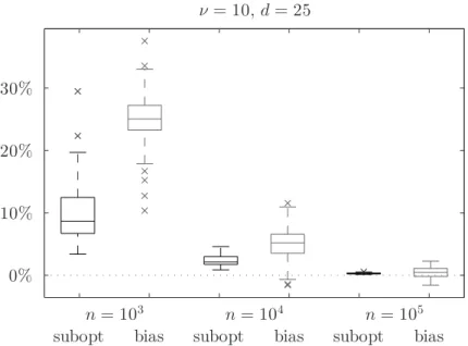
In Figure 1, the suboptimality and bias is plotted for different sample sizes n in the case τ= 0.999, ν = 10, and d= 25. The boxplot shows the range of the results over 100 runs, each based on an MC sample of n ob-servations of the asset returns vector. We observe that the bias (underestimation) is typically larger than sub-optimality, which means that the perceived expectile is often lower than the true optimum, while the actual expectile of the selected portfolio is higher than the optimum. Sometimes, however, the perceived expectile can be higher than the actual expectile of the selected portfolio (negative underestimation), but suboptimal-ity is always positive (above the dotted line). For sample size n= 1000, the suboptimality is typically around 10 %, but it can reach up to 30 %. Similar observations apply also for a lower expectile level, τ= 0.99; see Table 3, where the median and the 90th percentile of the suboptimality is listed for different ν and d. Table 3 also shows that the suboptimality is higher when the number of assets d is large and when the asset returns distribution is more heavy-tailed (lower parameter ν). In these cases, the suboptimality exceeds 10 %. Clearly, higher sample sizes are required to obtain portfolios that are closer to the optimum, as indicated by Figure 1.
n= 103 n= 104 n= 105
0% 10% 20% 30%
subopt bias subopt bias subopt bias
ν = 10, d = 25
Figure 1. Suboptimality of the LP solution portfolio expectile (black), and underestimation of its true expectile (gray), both relative to the optimal expectile. For each sample size n ∈ {103, 104, 105}, the boxplot shows the spread of the results
50th percentile 90th percentile d d ν 3 5 10 25 50 101 3 5 10 25 50 101 ∞ 0.4 0.7 1.9 3.4 4.5 5.4 1.1 1.7 3.2 4.6 6.0 7.3 10 0.7 1.2 2.6 4.6 5.7 7.8 1.7 1.9 4.0 6.5 8.1 10.6 5 0.7 2.2 3.3 5.9 8.2 9.4 2.9 5.5 6.7 9.4 11.0 13.4 3 1.6 4.2 6.4 8.6 11.3 13.4 4.9 11.9 13.6 14.1 17.5 18.5
Table 3. Portfolio suboptimality in percent of the optimal portfolio expectile at level τ = 0.99 with sample size n = 1000, depending on the number of assets d and Student-t parameter ν. The 50th and the 90th percentile of the outcomes in 100 experiment runs are listed.
50th percentile 90th percentile d d ν 3 5 10 25 50 101 3 5 10 25 50 101 ∞ 0.1 0.1 0.3 0.6 0.7 1.1 0.2 0.3 0.5 0.9 1.0 1.5 10 0.1 0.4 0.8 1.4 1.8 2.6 0.5 0.9 1.5 2.3 2.9 4.0 5 0.4 1.0 2.1 3.2 5.0 5.3 1.6 2.6 3.8 5.7 7.1 6.6 3 1.3 3.4 6.2 8.0 10.3 10.3 6.2 7.3 10.8 12.2 14.1 14.9
Table 4. Portfolio suboptimality in percent of the optimal portfolio expectile at level τ = 0.9999 with sample size n = 105,
depending on the number of assets d and Student-t parameter ν. The 50th and the 90th percentile of the outcomes in 100 experiment runs are listed.
In Table 4, the results with sample size n= 105for τ= 0.9999 are listed. For such a high expectile level, even an approximation with n= 105sample points may lead to portfolio suboptimality in excess of 10 %. Table 6 in the Appendix shows the results for the sample sizes that we considered as sufficient, namely,
n = 104for τ= 0.99, n = 105for τ= 0.999, and n = 106for τ= 0.9999. With these sample sizes, the subopti-mality of the selected portfolios was typically under 5 % even with a high number of assets and a heavy-tailed returns distribution. The LPs corresponding to the these sample sizes are computationally demanding to solve, because of the large number of decision variables and constraints. Therefore, it is important to use the most efficient (least time-consuming) LP formulation. This question is addressed in the next subsection.
3.2 Computation times
In this subsection, we analyze the computation times using the (Primal), (Dual) formulations, and the Aggre-gation algorithm for different problem instances corresponding to number of assets 3⩽ d ⩽ 101, Student-t parameter ν∈ {3, 5, 10, ∞}, and expectile levels τ ∈ {0.99, 0.999, 0.9999}. The computations were per-formed with IBM ILOG CPLEX 12.5, using Matlab interface on a 2.2 GHz AMD Opteron 6174. To estimate the computation times depending on the parameters ν, d, n and τ, for each combination, ten instances corresponding to ten MC samples of size n were solved using the three different formulations.
The two most common computational methods for solving LPs are the simplex algorithm and barrier (interior point) method. We compared the computation times for the three formulations using the two so-lution methods, and observed that, especially for the (Primal) and (Dual) formulations, the barrier method was considerably faster. This is consistent with the observations in the review paper by Gondzio [24] that “interior point methods are competitive when dealing with small problems of dimensions below one million constraints and variables and are beyond competition when applied to large problems of dimensions going into millions of constraints and variables”; see also [12].
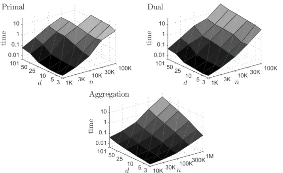
In Figure 2, the geometric average computation times (using the barrier method) for the (Primal), (Dual) formulations, and the Aggregation algorithm are plotted in a logarithmic scale against the number of assets d and sample size n. First, note that only with the Aggregation algorithm it was possible to solve instances
1K 3K 10K 30K 100K 3 5 10 25 50 101 0.01 0.1 1 10 n d ti m e
Primal
1K 3K 10K 30K 100K 3 5 10 25 50 101 0.01 0.1 1 10 n d ti m eDual
10K 30K 100K300K 1M 3 5 10 25 50 101 0.01 0.1 1 10 n d ti m eAggregation
Figure 2. Computation times in minutes for τ = 0.999, plotted in a logarithmic scale against d and n.
with sample size n> 105
with an average time of less than 45 minutes. We observe an approximately linear dependence (in the logarithmic scale) on d and n. To estimate the growth of the computation time in terms of d and n for each formulation and solution method, we fit a linear model for log-time (the input variables
d and n are on an approximately regular grid in the log-scale). This yields T(d, n) ≈ Cdanb
as a model for the computation time T in minutes. In Table 5, the fitted coefficients are listed. Note that to fit the parameters for the (Primal) and (Dual) formulations, we used 103⩽ n ⩽ 3 ⋅ 104for the simplex method and 103⩽ n ⩽ 105 for the barrier method. For the Aggregation algorithm, 3⋅ 104⩽ n ⩽ 106
were used for both methods. While the barrier method is clearly faster for the (Primal) and (Dual) formulations, the differences are less significant for the Aggregation algorithm, because the instances of (Aggregated) are of a much smaller size, where the two methods are competitive. Overall, for the considered levels τ and sample sizes in the thousands, the Aggregation algorithm is clearly the most efficient formulation, with computation times that are smaller than for the other two formulations by a factor of 50–200. The advantage increases as we consider larger sample sizes and higher expectile levels τ.
A further observation is that the parameter ν did not have a significant effect on the computation times using the (Primal) and (Dual) formulations. For the Aggregation algorithm, however, we see in Figure 3 that ν
Simplex Barrier τ a b T∗ a b T∗ 0.99 Primal 0.37 2.41 263 0.65 1.50 11.0 Dual 0.59 2.35 778 0.62 1.63 14.6 Aggregation 1.29 1.34 0.27 1.26 1.26 0.26 0.999 Primal 0.23 2.33 124 0.57 1.55 21.3 Dual 0.61 2.36 859 0.55 1.53 16.2 Aggregation 0.80 1.51 0.10 0.89 1.21 0.12 0.9999 Primal 0.10 2.18 68 0.61 1.51 23.2 Dual 0.61 2.37 905 0.48 1.52 21.2 Aggregation 0.66 1.32 0.07 0.65 1.10 0.07
Table 5. Fitted parameters to the model T = Cdanbfor computation time T in minutes. T∗is the fitted time for the
104 3 · 104 105 3 · 105 106 1s 5s 15s 1m 5m τ = 0.9999, d = 101 ν = ∞ ν = 10 ν = 5 ν = 3
Figure 3. Boxplot of computation times using the Aggregation algorithm for d = 101, τ = 0.9999, plotted in a logarithmic scale for different sample sizes n and Student-t distribution parameters ν.
has a significant effect, in particular, the cases with heavier tails (lower parameter ν) take less time. For example, with sample size n= 106and τ= 0.9999, the cases with normal distribution (ν = ∞) take 5 minutes on average, whereas with Student-t distributed returns (ν= 3) only 1.4 minutes. This is because the Aggre-gation algorithm is based on iteratively refining the partition of the scenarios into subsets that contain either only “good” or only “bad” outcomes. When the asset returns distribution is more heavy-tailed, it is easier to identify the outliers with large joint losses. This also explains why the Aggregation algorithm performs faster for high expectile levels τ: there are fewer “bad” scenarios to identify.
Remark 2. The conclusions regarding the three formulations for the expectile problem are somewhat differ-ent from those drawn in [26] for the CVaR problem. There, the dual formulation by [41] was considerably faster, because it replaced n joint constraints in the primal formulation of [43] with n constant bounds for the Radon–Nikodym derivatives, namely, φi⩽ 1/(1 − β), i = 1, . . . , n, according to the robust representation
of CVaRβ. In the case of the expectile, the constraints on φiare made dependent through m. This leads to similar growth rates O(n1.5) for the computation time in terms of n for both (Primal) and (Dual) algorithm (using the barrier method). Also, because of this inseparable set of n constraints for n+ 1 decision variables, scenario aggregation yields even greater relative savings in the computation time for the expectile problem.
4 Conclusions
In this paper, we considered the portfolio optimization problem where the risk is measured using the expec-tile. The expectile is a statistical functional that has recently gained attention due to its theoretical properties of coherence and elicitability, which make it an appealing candidate for use as a regulatory risk measure, as well as for managing portfolio risk. For elliptical joint asset returns distributions, the portfolio optimization problem with any coherent risk measure (such as the expectile) as the objective is solved by the minimal vari-ance portfolio. In contrast, for general asset returns distributions, the portfolio optimization problem may be very challenging. A practical method for obtaining close-to-optimal portfolios is approximating the true (respectively, modeled) continuous asset returns distribution using a discrete sample, and solving an LP for-mulation corresponding to the risk measure. In order to enable this approach for the expectile risk measure, we derived three LP formulations, which we refer to as primal, dual and Aggregation algorithm. In the numerical study, we observed that large samples (up to a million sample points) may be necessary to obtain a portfolio that is within 5 % of the optimum, especially for a high expectile level τ, a heavy-tailed asset returns distribution, and a large number of assets. The only formulation that was practical to use (in terms of the computation time) for solving problem instances of this size was the Aggregation algorithm. Also for lower sample sizes this algorithm offers a 50–200 times reduction in the computation time, compared to
the other two considered formulations. Overall, this paper confirms from another perspective that the expec-tile can be a useful risk measure, in particular, that it is possible to solve large scale portfolio optimization problems with the expectile objective.
Appendix
50th percentile 90th percentile d d ν 3 5 10 25 50 101 3 5 10 25 50 101 τ = 0.99, n = 104 ∞ 0.0 0.1 0.2 0.4 0.5 0.8 0.1 0.3 0.4 0.6 0.7 1.1 10 0.1 0.1 0.3 0.7 0.8 1.2 0.2 0.4 0.5 1.0 1.1 1.7 5 0.1 0.2 0.6 1.0 1.3 2.1 0.3 0.6 1.1 1.6 1.9 2.8 3 0.3 0.6 1.3 2.1 2.9 3.9 0.8 1.6 2.3 3.4 3.6 5.4 τ = 0.999, n = 105 ∞ 0.0 0.0 0.1 0.1 0.2 0.3 0.0 0.1 0.1 0.2 0.3 0.4 10 0.0 0.1 0.1 0.3 0.4 0.6 0.1 0.1 0.2 0.4 0.6 0.7 5 0.0 0.2 0.4 0.7 0.8 1.3 0.2 0.4 0.6 1.1 1.3 1.5 3 0.3 0.5 1.1 2.0 2.4 3.5 1.1 1.2 1.7 3.1 3.8 5.2 τ = 0.9999, n = 106 ∞ 0.0 0.0 0.1 0.2 0.3 0.4 0.0 0.1 0.1 0.3 0.4 0.5 10 0.0 0.0 0.1 0.2 0.3 0.5 0.1 0.1 0.2 0.4 0.5 0.6 5 0.1 0.1 0.3 0.6 0.7 1.1 0.2 0.3 0.6 0.7 1.0 1.6 3 0.1 0.5 1.0 2.0 2.6 3.4 0.6 0.9 2.0 3.0 4.7 4.7Table 6. Portfolio suboptimality in percent of the optimal portfolio expectile, depending on the expectile level τ, sample size n, Student-t parameter ν, and number of assets d. The 50th and the 90th percentile of the outcomes in 100 experiment runs are listed.
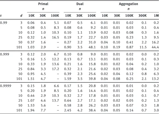
Primal Dual Aggregation
n n n τ d 10K 30K 100K 10K 30K 100K 10K 30K 100K 300K 1M 0.99 3 0.06 0.4 5.1 0.07 0.5 6.1 0.01 0.01 0.02 0.1 0.2 5 0.08 0.5 8.3 0.08 0.6 9.2 0.01 0.01 0.03 0.1 0.4 10 0.12 1.0 10.3 0.10 1.1 13.9 0.02 0.03 0.08 0.3 1.6 25 0.32 1.4 16.5 0.19 1.7 22.7 0.03 0.05 0.23 1.3 9.5 50 0.37 1.6 – 0.27 2.2 31.0 0.04 0.10 0.41 2.2 16.2 101 1.03 2.9 – 0.90 3.5 48.1 0.10 0.19 0.87 11.5 44.4 0.999 3 0.12 2.0 6.7 0.10 0.8 9.0 0.01 0.01 0.02 0.0 0.2 5 0.16 1.5 12.2 0.13 0.7 13.1 0.01 0.01 0.03 0.1 0.3 10 0.33 1.9 13.6 0.21 1.6 15.8 0.01 0.02 0.04 0.2 1.0 25 0.84 3.3 17.2 0.32 2.1 21.6 0.02 0.03 0.08 0.4 3.2 50 0.95 4.5 – 0.39 2.3 25.6 0.02 0.04 0.12 0.8 6.3 101 1.51 4.7 – 1.59 3.5 39.8 0.04 0.08 0.25 2.1 13.2 0.9999 3 0.15 1.8 6.6 0.17 1.5 20.8 0.01 0.01 0.01 0.0 0.2 5 0.20 1.9 8.5 0.20 1.6 14.4 0.01 0.01 0.02 0.1 0.4 10 0.44 2.9 10.3 0.32 2.7 17.8 0.01 0.01 0.03 0.1 0.7 25 1.07 4.6 13.7 0.64 2.7 17.1 0.02 0.02 0.05 0.2 1.3 50 1.53 5.6 – 0.58 2.8 26.2 0.03 0.03 0.07 0.3 1.8 101 1.94 7.7 – 2.45 4.2 38.4 0.04 0.05 0.14 0.7 3.0
Table 7. Geometric mean computation times (in minutes) of the optimal portfolio, depending on the expectile level τ, sample size n, and number of assets d. The LPs corresponding to the Primal, Dual, and Aggregation formulation were solved using the barrier method.
Acknowledgment: This work has benefited from stimulating discussions with Fabio Bellini and Christian Colombo during a visit to the University of Milano–Bicocca in January 2016.
Funding: The author gratefully acknowledges financial support from RiskLab Switzerland and the Swiss Finance Institute.
References
[1] K. Aas and I. Hobæk Haff, The generalized hyperbolic skew Student’s t-distribution, J. Financ. Econ.4 (2006), no. 2, 275–309.
[2] C. Acerbi and B. Szekely, Back-testing expected shortfall, Risk27 (2014), no. 11, 76–81.
[3] J. S. Ang, A note on the E, SL portfolio selection model, J. Financ. Quant. Anal.10 (1975), no. 05, 849–857. [4] P. Artzner, F. Delbaen, J.-M. Eber and D. Heath, Coherent measures of risk, Math. Finance9 (1999), no. 3, 203–228. [5] O. E. Barndorff-Nielsen, Exponentially decreasing distributions for the logarithm of particle size, Proc. Roy. Soc. Lond. A.
Math. Phys. Eng. Sci.353 (1977), no. 1674, 401–419.
[6] O. E. Barndorff-Nielsen, Normal inverse Gaussian distributions and stochastic volatility modelling, Scand. J. Stat.24 (1997), no. 1, 1–13.
[7] F. Bellini and V. Bignozzi, On elicitable risk measures, Quant. Finance15 (2015), no. 5, 725–733.
[8] F. Bellini, C. Colombo and M. Ç. Pınar, Portfolio optimization with expectiles, Poster presented at the workshop Dependence & Risk Measures, University of Milano–Bicocca, November 2015.
[9] F. Bellini and E. Di Bernardino, Risk management with expectiles, European J. Finance (2015), DOI 10.1080/1351847X.2015.1052150.
[10] F. Bellini, B. Klar, A. Müller and E. R. Gianin, Generalized quantiles as risk measures, Insurance Math. Econom.54 (2014), 41–48.
[11] A. E. Bernardo and O. Ledoit, Gain, loss, and asset pricing, J. Political Econ.108 (2000), no. 1, 144–172.
[12] R. E. Bixby, Solving real-world linear programs: A decade and more of progress, Oper. Res.50 (2002), no. 1, 3–15. [13] R. C. Blattberg and N. J. Gonedes, A comparison of the stable and Student distributions as statistical models for stock
prices, J. Bus.47 (1974), no. 2, 244–280.
[14] L. Carver, Mooted VaR substitute cannot be back-tested, says top quant, Risk2013 (2013). [15] L. Carver, Back-testing expected shortfall: Mission impossible?, Risk2014 (2014). [16] F. Delbaen, Monetary Utility Functions, Osaka University Press, Osaka, 2012.
[17] F. Delbaen, A remark on the structure of expectiles, preprint (2013), http://arxiv.org/abs/1307.5881.
[18] F. Delbaen, F. Bellini, V. Bignozzi and J. F. Ziegel, Risk measures with the CxLS property, Finance Stoch.20 (2016), no. 2, 433–453.
[19] G. De Rossi and A. Harvey, Quantiles, expectiles and splines, J. Econometrics152 (2009), no. 2, 179–185. [20] B. Efron, Regression percentiles using asymmetric squared error loss, Statist. Sinica1 (1991), no. 1, 93–125. [21] D. Espinoza and E. Moreno, A primal-dual aggregation algorithm for minimizing conditional-value-at-risk in linear
programs, Comput. Optim. Appl.59 (2014), no. 3, 617–638.
[22] H. Föllmer and A. Schied, Stochastic Finance: An Introduction in Discrete Time, Walter de Gruyter, Berlin, 2004. [23] T. Gneiting, Making and evaluating point forecasts, J. Amer. Statist. Assoc.106 (2011), no. 494, 746–762. [24] J. Gondzio, Interior point methods 25 years later, European J. Oper. Res.218 (2012), no. 3, 587–601. [25] J. Hull and A. White, Hull and White on the pros and cons of expected shortfall, Risk2014 (2014).
[26] E. Jakobsons, Suboptimality in portfolio conditional value-at-risk optimization, J. Risk18 (2016), no. 4, 1–23. [27] E. Jakobsons and S. Vanduffel, Dependence uncertainty bounds for the expectile of a portfolio, Risks3 (2015), no. 4,
599–623.
[28] P. Jorion, Value at Risk: The New Benchmark for Managing Financial Risk, McGraw–Hill, New York, 1996.
[29] M. Kapsos, S. Zymler, N. Christofides and B. Rustem, Optimizing the Omega ratio using linear programming, J. Comput.
Finance17 (2014), no. 4, 49–57.
[30] C. Keating and W. F. Shadwick, A universal performance measure, J. Perform. Measurement6 (2002), no. 3, 59–84. [31] H. Konno and H. Yamazaki, Mean-absolute deviation portfolio optimization model and its applications to Tokyo stock
market, Manag. Sci.37 (1991), no. 5, 519–531.
[32] C.-M. Kuan, J.-H. Yeh and Y.-C. Hsu, Assessing value at risk with CARE, the conditional autoregressive expectile models,
J. Econometrics150 (2009), no. 2, 261–270.
[33] D. B. Madan and E. Seneta, The variance gamma (VG) model for share market returns, J. Bus.63 (1990), no. 4, 511–524. [34] R. Mansini, W. Ogryczak and M. G. Speranza, LP solvable models for portfolio optimization: A classification and
[35] R. Mansini, W. Ogryczak and M. G. Speranza, Conditional value at risk and related linear programming models for portfolio optimization, Ann. Oper. Res.152 (2007), no. 1, 227–256.
[36] R. Mansini, W. Ogryczak and M. G. Speranza, Twenty years of linear programming based portfolio optimization, European
J. Oper. Res.234 (2014), no. 2, 518–535.
[37] R. Mansini, W. Ogryczak and M. G. Speranza, Linear and Mixed Integer Programming for Portfolio Optimization, Springer, Cham, 2015.
[38] H. Markowitz, Portfolio selection, J. Finan.7 (1952), no. 1, 77–91.
[39] A. J. McNeil, R. Frey and P. Embrechts, Quantitative Risk Management: Concepts, Techniques and Tools, Princeton University Press, Princeton, 2005.
[40] W. K. Newey and J. L. Powell, Asymmetric least squares estimation and testing, Econometrica55 (1987), no. 4, 819–847. [41] W. Ogryczak and T. Śliwiński, On solving the dual for portfolio selection by optimizing conditional value at risk, Comput.
Optim. Appl.50 (2011), no. 3, 591–595.
[42] B. Rémillard, Statistical Methods for Financial Engineering, CRC Press, Boca Raton, 2013.
[43] R. T. Rockafellar and S. Uryasev, Optimization of conditional value-at-risk, J. Risk2 (2000), no. 3, 21–42.
[44] W. F. Sharpe, A linear programming approximation for the general portfolio analysis problem, J. Financ. Quant. Anal.6 (1971), no. 5, 1263–1275.
[45] Q. Yao and H. Tong, Asymmetric least squares regression estimation: A nonparametric approach, J. Nonparametr. Stat.6 (1996), no. 2–3, 273–292.
[46] J. F. Ziegel, Coherence and elicitability, Mathematical Finance (2014), DOI 10.1111/mafi.12080.
[47] Basel Committee on Banking Supervision, Fundamental review of the trading book, 2012, available at www.bis.org/publ/ bcbs219.htm.