1
Appendix
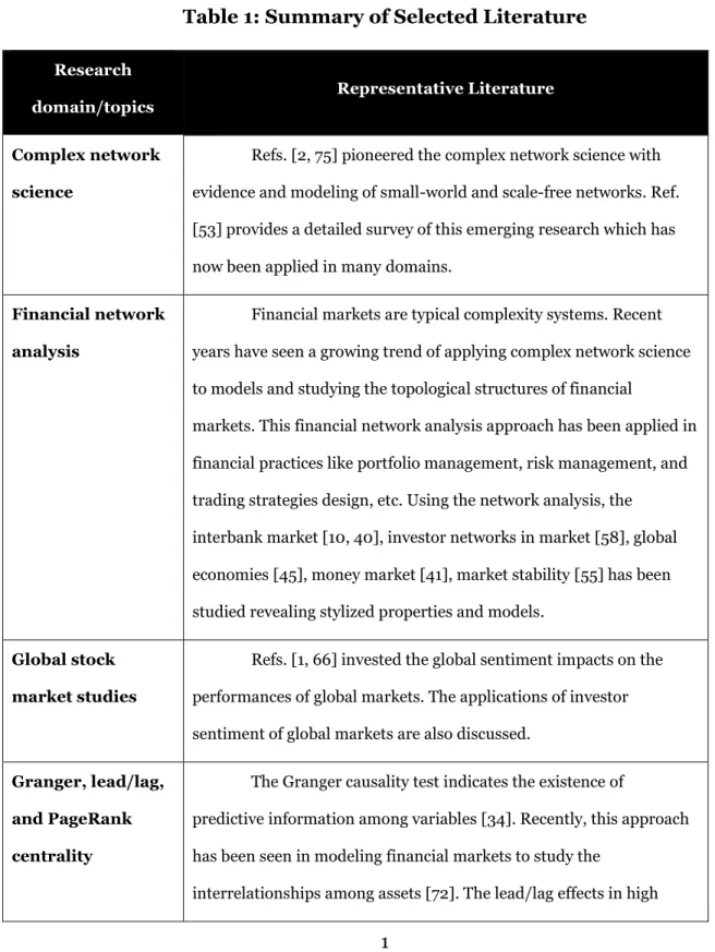
Table 1: Summary of Selected Literature
Research
domain/topics Representative Literature
Complex network science
Refs. [2, 75] pioneered the complex network science with evidence and modeling of small-world and scale-free networks. Ref. [53] provides a detailed survey of this emerging research which has now been applied in many domains.
Financial network
analysis
Financial markets are typical complexity systems. Recent years have seen a growing trend of applying complex network science to models and studying the topological structures of financial
markets. This financial network analysis approach has been applied in financial practices like portfolio management, risk management, and trading strategies design, etc. Using the network analysis, the
interbank market [10, 40], investor networks in market [58], global economies [45], money market [41], market stability [55] has been studied revealing stylized properties and models.
Global stock market studies
Refs. [1, 66] invested the global sentiment impacts on the performances of global markets. The applications of investor sentiment of global markets are also discussed.
Granger, lead/lag, and PageRank centrality
The Granger causality test indicates the existence of
predictive information among variables [34]. Recently, this approach has been seen in modeling financial markets to study the
2
frequency data are investigated in [39, 44].
Refs. [12, 21] provide more evidence of lead/lag in global markets. These empirical findings reveal the stylized lead/lag effects exist in various markets and implicate possible applications in trading, for example, possible trading based on the lead/lag between index and derivatives like futures. PageRank algorithm is first proposed to quantitatively evaluate the importance of network vertices [59]. To compare with other metrics of centrality like degree, between-ness, etc., in the similar spirit, the alternative of eigenvector centrality, PageRank centrality is widely used to calculate the
3
Granger Causality and Data
Granger Causality
The stocks in the market not only fluctuate correlatively but also influence with each other. This applies to the global financial market as well, where different stock markets have significant impacts with each other. Based on the correlation matrix generated from the price return series of a set of stocks, correlation of two stocks 𝑠𝑖 and 𝑠𝑗, can be defined as
𝜌𝑖𝑗 =
〈𝑌𝑖𝑌𝑗〉−〈𝑌𝑖〉〈𝑌𝑗〉
√(〈𝑌𝑖2〉−〈𝑌𝑖〉2)(〈𝑌𝑗2〉−〈𝑌𝑗〉2)
. (1)
Eq. 1 shows how the two series 𝑌𝑖 and 𝑌𝑗 of stock 𝑆𝑖 and 𝑆𝑗 co-move with
each other. Since −1 ≤ 𝜌𝑖𝑗 ≤ 1, the two series can move in the same direction or
the opposite based on the sign of 𝜌𝑖𝑗. It is thus possible to evaluate the collective
behaviors of a pair of stocks or a set of stocks in a given portfolio.
However, the shortcomings of correlation-based approaches are apparent. The primary issue is that the correlations do not give statistical information of the causality between stock pairs. Due to this, the correlation approach lacks the ability in describing the lead/lag behaviors of stocks. Correlation information only reveals the pattern of movements of two series but fails to explain the causal relationships. In the real world, two phenomena, especially those happening along time, often have specific cause/effect relationship. For example, 𝐴 has an influence over 𝐵 or 𝐴 contributes certain causality to the happening or effects of 𝐵.
4
A set of stocks in a given portfolio are not only co-moving with each other, but also have mutual influence with each other. Some stocks can cause other stocks to change. Unfortunately, the correlation method fails to explain. Thus, new measurements beyond the correlations to provide causality information between pairs with statistical meanings are needed.
To describe the aspect of causalities between events, the Granger causality test was introduced by Granger [34]. The hypothesis test is setup in evaluating the predictive ability between variables in a context of linear regressions. There are two time series 𝑥𝑡, 𝑥𝑡−1, … , 𝑥0, and 𝑦𝑡, 𝑦𝑡−1, … , 𝑦0 over a
time period of 𝑡 = 0, 1, … , 𝑇. A linear regression can be set up as:
𝑦𝑡 = ∑𝑞𝑖=1𝛼𝑖𝑥𝑡−𝑖+ ∑𝑞𝑗=1𝛽𝑗𝑦𝑡−𝑗+ 𝑢𝑡1 , (2)
and similarly,
𝑥𝑡 = ∑𝑠𝑖=1𝛾𝑖𝑥𝑡−𝑖+ ∑𝑠𝑗=1𝜆𝑗𝑦𝑡−𝑗+ 𝑢𝑡2, (3)
where 𝑢𝑡1 and 𝑢𝑡2 are independent white noises. These regressions take the
previous behaviors of both 𝑥𝑡 and 𝑦𝑡 into consideration to predict the present
values.
The null hypothesis can be set up as:
𝐻0: 𝛼1 = 𝛼2 = ⋯ = 𝛼𝑞= 0 for Eq. 2, and 𝜆1 = 𝜆2 = ⋯ = 𝜆𝑠 = 0 for Eq. 3.
The alternative hypothesis can be set up as:
5
The statistical philosophy behind the Granger test is that if the lagged values of 𝑥 together with its values of 𝑦 is included, it enables us to get a better prediction of the future values of 𝑦 than without the help of lagged 𝑥 values, then 𝑥 Granger-causes 𝑦. Otherwise, if the lagged values of 𝑥 fail to contribute in the prediction of future 𝑦, then x does not Granger-cause 𝑦. It is also the same if 𝑦 Granger causes 𝑥.
To conduct hypothesis testing, the F-test will be utilized. Taking the two 𝐻0 for both Eq. 2 and Eq. 3 all together, there are four scenarios:
1. 𝑥𝑡 unidirectional Granger causes 𝑦𝑡, i.e. 𝛼𝑖 ≠ 0 and 𝜆𝑗 = 0; 2. 𝑦𝑡 unidirectional Granger causes 𝑥𝑡, i.e. 𝜆𝑗 ≠ 0 and 𝛼𝑗 = 0;
3. 𝑥𝑡 and 𝑦𝑡 bidirectional cause each other, i.e. 𝛼𝑖 ≠ 0 and 𝜆𝑗 ≠ 0;
4. 𝑥𝑡 and 𝑦𝑡 are independent, i.e. 𝛼𝑗 = 0 and 𝜆𝑗 = 0.
ADF and Unit Root Test
Before the Granger causality test is conducted, it is important to make sure the time series are stationary. This is done by conducting a unit root test. The Dickey-Fuller test [65] is usually applied to test the unit root; an extension is further developed as Augmented Dickey-Fuller (ADF) test. In ADF, a t-statistic can be compared with critical values on different levels of statistical significances. If the t-statistic is larger, then we do not reject the null hypothesis that a unit root exists. In this case, the time series is not stationary. Otherwise, we reject the
6
null hypothesis and believe that the time series is stationary and fits to conduct ADF. For stock returns, an event can bring certain impact into the fluctuations to the series, but this impact will decay allowing the return back to its mean.
Granger causality test has become a standard tool in the study of the causality relationships for pairs. With these pairs of causality information, a causality network for a set of variables can be constructed. Given the time lag nature of Granger test, it has become widely used in economics and finance studies [24].
Data Setting Introduction
The causalities among financial series is discussed in this section. Based on these tests, the Granger-causality networks are built, and the properties of these networks are investigated.
The daily close data for 33 major stock market indices around the world in the period of 04/01/2007 to 06/11/2015 with 2307 total trading dates from Yahoo Finance was collected in this research. Since each stock market has its trading calendar with different holidays and closed dates, the missing dates were replaced with the next available data. There are discussions of the time-zone effect in study of global indices because of the different closing time for each market. However, we concern the closing prices in an extended period and treat all indices in the same way. This approach focuses on the closing prices without special procession of adjusting. For each index, the log return is applied as:
7
𝑌𝑖 = 𝑙𝑛 𝑃𝑖(𝑡) − 𝑙𝑛 𝑃𝑖(𝑡 − 1), (4)
where 𝑃𝑖(𝑡) is the closing price for index 𝑖 at time 𝑡. In Table 2, all 33 indices
utilized in this study are listed. It represents major stock markets, including 4 from the US, 12 from Europe countries, 11 from Asian countries, 5 American countries and one Middle Eastern country. In Fig. 1, log daily returns for all indices over the study period is plotted. The returns demonstrate fluctuation but the means are around zero. ADF tests over all return time series were conducted. The average t-statistic is larger than all 6 critical values (in absolute value terms) at significance levels of 1%, 5%, 10%, 90%, 95%, and 99%. In fact, t-statistic ranges from -20.4871 to -17.5458, suggesting all return series are stationary. This aligns with the visualizations, that all return series move around the mean of zero. With this stationary background, the Granger causality test can be carried out later.
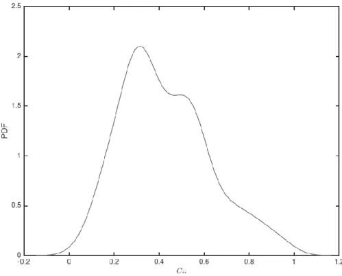
We first use all logged return data over the whole study period to construct the correlation matrix 𝐶𝑖𝑗. This approach is widely adopted in financial network
analysis to convert price or return time series data into correlation matrices [13, 53, 54]. We plot the probability density function (PDF) to show the distribution of 𝐶𝑖𝑗 of all indices calculated from the data over the whole study period in Fig. 2.
The average correlation 𝜌𝑖𝑗 = 0.4269 with standard deviation 𝜎𝑖𝑗 = 0.1963. Since
the average correlation is positive, all indices co-move together. We also observe that a maximum 𝑚𝑎𝑥(𝜌𝑖𝑗) = 0.9858 for S&P500 and NYSE, 𝑚𝑖𝑛(𝜌𝑖𝑗) = 0.0337
8
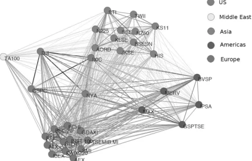
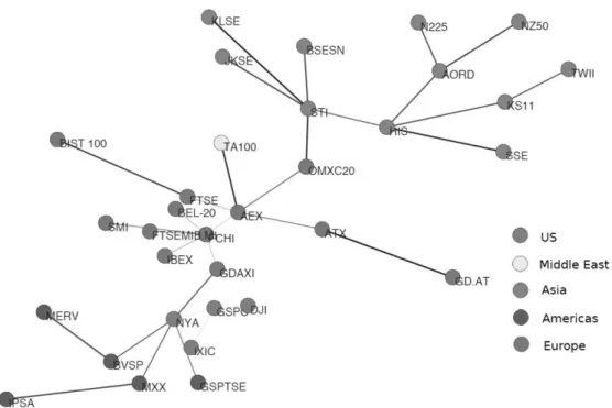
for NASDAQ and NZ50 (New Zealand). Based on the correlation information, the complete graph of the indices network in Fig. 3 provides the backbone of the full network. Furthermore, the minimum spanning tree MST is provided in Fig. 4, where markets of the same regions are clearly identified.
9
Table 2: Tick names, markets, countries and regions of 33 major stock markets indices around the world.
Tick Name Country Region
GSPC S&P 500 US America
DJI Dow Jones Industrial Average US America
IXIC NASDAQ Composite US America
NYA NYSE Composite US America
FTSE FTSE 100 UK Europe
GDAXI DAX Germany Europe
FCHI CAC 40 France Europe
ATX ATX Austria Europe
GD.AT Athen Index Compos Greece Europe
IBEX IBEX 35 Spain Europe
FTSEMIB.MI FTSE MIB Italy Europe
SMI Swiss Market Index Switzerland Europe
OMXC20 OMX Copenhagen 20 Denmark Europe
AEX Amsterdam Exchange index Netherlands Europe
BEL-20 EURONEXT BEL-20 Belgium Europe
BIST 100 XU100 Turkey Europe
N225 Nikkei 225 Japan Asia
HSI Hang Seng Index Hong Kong Asia
SSE SSE Composite Index China Asia
STI STI Index Singapore Asia
AORD ALL ORDINARIES Australian Asia
BSESN S&P BSE SENSEX India Asia
JKSE Jakarta Composite Index Indonesia Asia
KLSE FTSE Bursa Malaysia KLCI Malaysia Asia
NZ50 S&P/NZX 50 Index Gross New Zealand Asia
KS11 KOSPI Composite Index Korea Asia
TWII TSEC weighted index Taiwan Asia
GSPTSE S&P/TSX Composite index Canada Americas
BVSP IBOVESPA Brazil Americas
MXX IPC Mexico Americas
IPSA IPSA Santiago de Chile Chile Americas
MERV MerVal Buenos Aires Argentina Americas
10
Figure 1: The daily log returns of 33 major market indices around the world. It shows the returns volatiles over our study period between 04/01/2007 and 06/11/2015 covering a total of 2307 trading dates. They are all stationary with means around zero.
11
Figure 2: The probability density function (PDF) of correlations of all indices over the whole study period. The distribution falls on the right side of zero indicating that the indices are positively correlated. In other words, they are influencing each other.
12
Figure 3: The correlation based network of 33 indices calculated from the daily return data over the whole study period.
13
Figure 4: The minimum spanning tree MST extracted from the full network of 33 indices calculated from the daily return data over the whole study period. We see the indices are clustered together according to the regions.