HAL Id: hal-00295706
https://hal.archives-ouvertes.fr/hal-00295706
Submitted on 3 Aug 2005
HAL is a multi-disciplinary open access
archive for the deposit and dissemination of
sci-entific research documents, whether they are
pub-lished or not. The documents may come from
teaching and research institutions in France or
abroad, or from public or private research centers.
L’archive ouverte pluridisciplinaire HAL, est
destinée au dépôt et à la diffusion de documents
scientifiques de niveau recherche, publiés ou non,
émanant des établissements d’enseignement et de
recherche français ou étrangers, des laboratoires
publics ou privés.
measurement and 1-D simulations for cloudless, broken
cloud and overcast situations
A. Kylling, A. R. Webb, R. Kift, G. P. Gobbi, L. Ammannato, F. Barnaba, A.
Bais, S. Kazadzis, M. Wendisch, E. Jäkel, et al.
To cite this version:
A. Kylling, A. R. Webb, R. Kift, G. P. Gobbi, L. Ammannato, et al.. Spectral actinic flux in the lower
troposphere: measurement and 1-D simulations for cloudless, broken cloud and overcast situations.
Atmospheric Chemistry and Physics, European Geosciences Union, 2005, 5 (7), pp.1975-1997.
�hal-00295706�
SRef-ID: 1680-7324/acp/2005-5-1975 European Geosciences Union
Chemistry
and Physics
Spectral actinic flux in the lower troposphere: measurement and
1-D simulations for cloudless, broken cloud and overcast situations
A. Kylling1, A. R. Webb2, R. Kift2, G. P. Gobbi3, L. Ammannato3, F. Barnaba3, A. Bais4, S. Kazadzis4, M. Wendisch5, E. J¨akel5, S. Schmidt5, A. Kniffka6, S. Thiel7, W. Junkermann7, M. Blumthaler8, R. Silbernagl8, B. Schallhart8, R. Schmitt9, B. Kjeldstad10, T. M. Thorseth10, R. Scheirer11, and B. Mayer11
1Norwegian Institute for Air Research, Kjeller, Norway; now at St. Olavs Hospital, Trondheim University Hospital, Norway 2Physics Department, University of Manchester Institute of Science and Technology, Manchester, UK
3Istituto di Scienze dell’Atmosfera e del Clima-CNR, Roma, Italy
4Laboratory of Atmospheric Physics Aristotle University of Thessaloniki, Greece 5Leibniz-Institut f¨ur Troposph¨arenforschung, Leipzig, Germany
6Institut f¨ur Meteorologie, Universit¨at Leipzig, Leipzig
7Institut f¨ur Meteorologie und Klimaforschung, Garmisch-Partenkirchen, Germany 8Institute of Medical Physics, University of Innsbruck, Innsbruck, Austria
9Meteorologie Consult GmbH, Germany
10Department of Physics, Norwegian University of Science and Technology, Trondheim 11Deutsches Zentrum f¨ur Luft- und Raumfahrt (DLR), Oberpfaffenhofen, Wessling, Germany
Received: 25 January 2005 – Published in Atmos. Chem. Phys. Discuss.: 10 March 2005 Revised: 21 June 2005 – Accepted: 27 June 2005 – Published: 3 August 2005
Abstract. In September 2002, the first INSPECTRO
cam-paign to study the influence of clouds on the spectral ac-tinic flux in the lower troposphere was carried out in East Anglia, England. Measurements of the actinic flux, the irra-diance and aerosol and cloud properties were made from four ground stations and by aircraft. The radiation measurements were modelled using the uvspec model and ancillary data. For cloudless conditions, the measurements of the actinic flux were reproduced by 1-D radiative transfer modelling within the measurement and model uncertainties of about
±10%. For overcast days, the ground-based and aircraft ra-diation measurements and the cloud microphysical property measurements are consistent within the framework of 1-D radiative transfer and within experimental uncertainties. Fur-thermore, the actinic flux is increased by between 60–100% above the cloud when compared to a cloudless sky, with the largest increase for the optically thickest cloud. Correspond-ingly, the below cloud actinic flux is decreased by about 55– 65%. Just below the cloud top, the downwelling actinic flux has a maximum that is seen in both the measurements and the model results. For broken clouds the traditional cloud frac-tion approximafrac-tion is not able to simultaneously reproduce the measured above-cloud enhancement and below-cloud re-duction in the actinic flux.
Correspondence to: A. Kylling
1 Introduction
Clouds exhibit large variations in their optical properties on both small and large scales. Furthermore, their shapes have an infinite multitude of realisations. Thus, due to their na-ture, clouds are a challenge to treat realistically in radiative transfer calculations. Clouds are important for the radiative energy budget of the Earth (Ramanathan et al., 1989), and they influence the amount of radiation available for photo-chemistry (Madronich, 1987). For example, the reflection of radiation by clouds shifts the photostationary state rela-tionship (NO-O3-NO2) towards NO, thereby favoring NO to
NO2 conversions by other compounds than O3. This
effec-tively increases O3formation rate in the upper troposphere.
Other photolysis rates are affected as well, and these changes may either add to or counteract to the chemical effect of en-hanced NO2photolysis (Thompson, 1984). Clouds may also
both decrease and increase the amount of biologically harm-ful UV irradiance at Earth’s surface (e.g. Mims and Freder-ick, 1994).
The simplest way to introduce clouds in radiative trans-fer models is to approximate them as a single, homogeneous layer. This approach is and has been used for a number of studies. The limitation of this approximation is evident, es-pecially when considering broken-cloud conditions. How-ever, apparently horizontally homogeneous clouds may ex-hibit large variations, and the corresponding radiative effects may locally be large (Cahalan et al., 1994).
Experimental investigations of the effect of clouds on the radiation which are of importance for the photochemistry of the atmosphere have been carried out by several groups. Many of these have measured the photolysis frequencies J(O1D) and J(NO2), while rather few have investigated the
spectral actinic flux. The spectral actinic flux is needed to calculate the photolysis frequency (Madronich, 1987) and is also the quantity calculated by radiative transfer models used in photochemistry applications.
The J(O1D) photolysis frequency was measured by Junkermann (1994) from a hangglider above snow surfaces and within and above stratiform clouds. The photolysis fre-quency increased by a factor of 2 above the cloud com-pared to cloudless conditions. Snow on the ground increased the cloudless photolysis frequency, with the increase being largest for conditions with high visibility. Vil`a–Guerau de Arellano et al. (1994) made tethered-balloon measurements of the actinic flux integrated between 330 and 390 nm in cloudy conditions. They found excellent agreement between a delta-Eddington radiative transfer model and the measure-ments during overcast conditions. For partial cloudiness (≤7 oktas), there was a larger disagreement between the mea-surements and the model simulations (their Fig. 2). Kel-ley et al. (1995) reported actinometer measurements of the J(NO2) photolysis frequency during cloudless and cloud
con-ditions. They reported a J(NO2) in-cloud enhancement of
up to 58%. The effect of clouds on J(NO2) was also
dis-cussed by Lantz et al. (1996), and they proposed a simpli-fied cloud model to explain J(NO2) values that exceeded
clear sky values during partly cloudy conditions. Matthi-jsen et al. (1998) converted UV irradiance aircraft measure-ments to J(O1D) photolysis frequencies. They subsequently used cloud microphysical measurements and radiative trans-fer calculations to investigate the effect of clouds on the pho-tolysis frequency J(O1D) and the OH concentration. The modelled profile of OH was compared with measurements and generally good agreement was found for rather complex cloud conditions. Fr¨uh et al. (2000) compared aircraft mea-surements of J(NO2) with model simulations for clear and
cloudless situations for altitudes up to 2.5 km. Cloud input to the model was provided by simultaneous measurements of thermodynamic, aerosol particle, and cloud drop properties. For the cases studied, cloudless and total cloud cover, the measurements and model simulations agreed to within 10%. Shetter and M¨uller (1999) made measurement of the spectral actinic flux, which was used to calculate various photolysis frequencies. For flights over the Pacific Ocean, photolysis frequency enhancements due to clouds of about a factor of 2 over cloudless values were reported. Crawford et al. (2003) and Monks et al. (2004) investigated the cloud impacts on surface UV spectral actinic flux during cloudless and cloudy situations. Wavelength-dependent enhancements and reduc-tions compared to a cloudless sky were observed when dur-ing partial cloud cover the sun is unobscured and obscured, respectively.
On the theoretical side, numerous model studies have in-vestigated the 3-D effects of clouds. Most of these have focused on cloud albedo and energy budget studies, cloud absorption anomaly (Stephens and Tsay, 1990) and satellite retrievals (Chambers et al., 1997). Also, they mostly ex-amine how inhomogeneities change radiance and flux val-ues at fixed locations. A more generally descriptive frame-work has been developed by V´arnai and Davies (1999), who consider how individual photons are influenced by hetero-geneities as they move along their paths within a cloud layer. Rather few studies have looked at the effect on the actinic flux. The first study of 3-D cloud effects on the actinic flux was made by Los et al. (1997). They considered hexagonal clouds for various cloud fractions with a Monte Carlo model. Molecular and aerosol scattering was not included in their simulations. Trautmann et al. (1999) investigated the spatial distribution of the actinic flux for 2D clouds in an aerosol-free atmosphere with both a Monte Carlo model and the Spherical Harmonic Discrete Ordinate Method (SHDOM, Evans, 1998). Among their conclusions was the finding that the plane-parallel approximation generally underestimates the photodissociation coefficients in and below the cloud. Brasseur et al. (2002) performed 3-D model investigations of the impact of a deep convective cloud on photolysis fre-quencies and photochemistry. The radiative impacts were quantified with SHDOM, and enhancement factors of the lo-cal spectral actinic flux relative to the incoming flux were calculated. Increases of the actinic flux relative to the in-coming flux of 2 to 5, compared to cloudless values, were found above, at the top edge and around the deep convective cloud. This enhanced actinic flux produced enhanced OH concentrations (120–200%) in the upper troposphere above the clouds and changes in ozone production (+15%). It is noted that the full 3-D radiative transfer problem may be solved by a number of different methods. While all are computationally demanding, the 3-D problem is nevertheless solvable. The main challenge with 3-D radiative transfer in the presence of clouds is to specify the cloud input.
The earlier experimental studies of the influence of clouds on the actinic flux and photolysis frequencies have either been part of a larger campaign with a different main focus and/or been performed by a single platform. As part of the in-fluence of clouds on the spectral actinic flux in the lower tro-posphere (INSPECTRO) project, a dedicated measurement campaign was carried out with the aim to characterize the cloud, aerosol and radiation within a well defined area. In the following, the measurements are described first, followed by a brief description of the radiative transfer model used for the data interpretation. The method used to derive a cloud opti-cal depth is discussed next. This is followed by a discussion of the measured and simulated spectral actinic fluxes under cloudless, overcast and broken cloud conditions. Finally the paper is summarized.
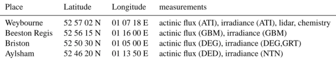
Table 1. Location of the ground stations and the type of measurements made at the respective stations. For description of the instrumentation
see Table 2.
Place Latitude Longitude measurements
Weybourne 52 57 02 N 01 07 18 E actinic flux (ATI), irradiance (ATI), lidar, chemistry Beeston Regis 52 56 15 N 01 16 00 E actinic flux (GBM), irradiance (GBM)
Briston 52 50 30 N 01 05 00 E actinic flux (DEG), irradiance (DEG,GRT) Aylsham 52 46 20 N 01 13 50 E actinic flux (DED), irradiance (NTN)
2 Measurements
The INSPECTRO campaign took place in East Anglia, Eng-land, September 2002. It began with a one-week intercom-parison of all radiation instrumentation at the Weybourne sta-tion. The following three weeks the instruments were in op-eration at four different stations located such as to cover a grid of approximately 12×12 km2, see Table 1.
Aircraft measurements were carried out on 11 of the to-tal of 20 campaign days. A list over all instruments utilized in the present study is given in Table 2. Further details are provided below.
2.1 Ground measurements
Ground measurements were made at four locations north-east of the international airport of Norwich. Two of the sta-tions, Briston and Aylsham, were inland, while the other two, Weybourne and Beeston Regis, were on the coast (see Ta-ble 1). All stations made irradiance and downwelling ac-tinic flux measurements. Both scanning and diode array spectrometers were in use (see Table 2). The instruments and their calibration have been described earlier in connec-tion with the actinic flux determinaconnec-tion from measurements of irradiance (ADMIRA) project by Webb et al. (2002) and references therein. At the start of the campaign, an instru-ment comparison was performed in Weybourne with all in-struments present. The Joint Research Centre (JRC) travel-ling reference spectroradiometer performed irradiance mea-surements during the intercomparison and also travelled to all locations afterwards to check the stability of each instru-ment and the possible effects of transportation. Typically, the agreement between the various independently calibrated instruments was within ±10%, which is within their mea-surement uncertainties of about ±5%.
At Weybourne the Vehicle-Mounted Lidar System (Gobbi et al., 2000, VELIS) was in operation throughout the cam-paign. Measurements from VELIS were used to retrieve the aerosol backscatter and extinction profiles at 532 nm using the methods described in Gobbi et al. (2004) and Barnaba and Gobbi (2004). These aerosol optical properties were used as input to radiative transfer simulations. In addition, VELIS provided cloud bottom altitude and cirrus cloud in-formation.
2.2 Airborne platforms
During the INSPECTRO campaign, the Partenavia P68C air-craft operated by the Leibniz-Institute for Tropospheric Re-search (IfT) measured the downwelling and upwelling irra-diances and actinic fluxes. The irrairra-diances are measured by the so-called Albedometer (Wendisch et al., 2001; Wendisch and Mayer, 2003; Wendisch et al., 2004). The actinic fluxes are measured by the actinic flux density meter (AFDM) de-scribed by J¨akel et al. (2005). In addition to the radiation in-strumentation, the IfT-Partenavia has various instruments for measurement of particle size distribution and concentrations. A Particle Volume Monitor (PVM) was used to measure the liquid water content, with an error of about ±10%. The wa-ter droplet effective radius, defined as the ratio of the third to the second moment of the droplet size distribution, was deduced from Fast Forward Scattering Spectrometer Probe (Fast-FSSP) measurements, with an error of about ±4%. Fi-nally, the aircraft was equipped with sensors for measure-ment of standard avionic and meteorological parameters.
Albedo measurements in the UV and visible were per-formed by the Cessna 182 light aircraft from the Univer-sity of Manchester Institute of Science and Technology. A temperature-stabilised Optronic 742 wavelength-scanning spectroradiometer measured the up- and downwelling irra-diances at selected wavelengths. From the irradiance mea-surements at various altitudes, the albedo of the surface be-low was derived. In addition, the albedo at 312 and 340 nm was deduced from measurements of the NILU-CUBE instru-ment (Kylling et al., 2003a) suspended below a hot air bal-loon. These albedo measurements are described by Webb et al. (2005).
3 Radiative transfer model
The uvspec model from the libradtran package (http://www. libradtran.org and Mayer and Kylling , 2005) was used to simulate the measurements. Input to the model are profiles of the atmosphere taken from the U.S. standard atmosphere (Anderson et al., 1986). The aerosol optical depth pro-file was taken from the VELIS measurements. The aerosol single-scattering albedo and asymmetry factor were set to 0.98 and 0.75, respectively. Changes in the solar zenith angle during a single measurement scan are accounted for.
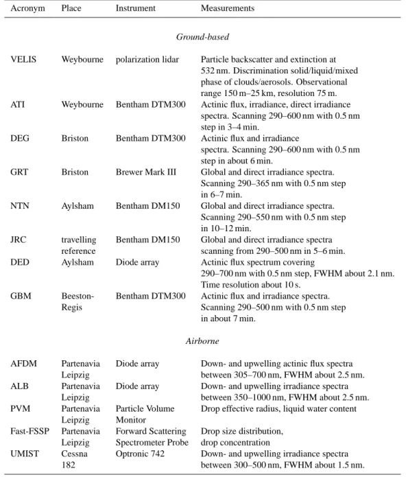
Table 2. Instruments located at the various stations. Additional instrumentation were also present, but not used in this study.
Acronym Place Instrument Measurements
Ground-based
VELIS Weybourne polarization lidar Particle backscatter and extinction at 532 nm. Discrimination solid/liquid/mixed phase of clouds/aerosols. Observational range 150 m–25 km, resolution 75 m. ATI Weybourne Bentham DTM300 Actinic flux, irradiance, direct irradiance
spectra. Scanning 290–600 nm with 0.5 nm step in 3–4 min.
DEG Briston Bentham DTM300 Actinic flux and irradiance
spectra. Scanning 290–600 nm with 0.5 nm step in about 6 min.
GRT Briston Brewer Mark III Global and direct irradiance spectra. Scanning 290–365 nm with 0.5 nm step in 6–7 min.
NTN Aylsham Bentham DM150 Global and direct irradiance spectra. Scanning 290–550 nm with 0.5 nm step in 10–12 min.
JRC travelling Bentham DM150 Global and direct irradiance spectra reference scanning from 290–500 nm in 5–6 min. DED Aylsham Diode array Actinic flux spectrum covering
290–700 nm with 0.5 nm step, FWHM about 2.1 nm. Time resolution about 10 s.
GBM Beeston- Bentham DTM300 Actinic flux and irradiance spectra. Regis Scanning 290–500 nm with 0.5 nm step
in about 7 min.
Airborne
AFDM Partenavia Diode array Down- and upwelling actinic flux spectra Leipzig between 305–700 nm, FWHM about 2.5 nm. ALB Partenavia Diode array Down- and upwelling irradiance spectra
Leipzig between 350–1000 nm, FWHM about 2.5 nm. PVM Partenavia Particle Volume Drop effective radius, liquid water content
Leipzig Monitor
Fast-FSSP Partenavia Forward Scattering Drop size distribution, Leipzig Spectrometer Probe drop concentration
UMIST Cessna Optronic 742 Down- and upwelling irradiance spectra 182 between 300–500 nm, FWHM about 1.5 nm.
Temperature-dependent ozone cross sections are taken from Bass and Paur (1985). The ozone column was taken either from the GRT Brewer instrument or the Earth Probe To-tal Ozone Monitoring Spectrometer (TOMS) (Table 3). The ozone column was assumed to be constant over the measure-ment area. For days 257 and 261 the TOMS total ozone col-umn was used as clouds prevented measurements with the GRT Brewer. For the other days the GRT measurements were utilized. The uncertainty in the total ozone column measurements are about 2% for the Brewer under cloudless conditions and about 4% for the TOMS. The ozone mea-surement did not always coincide in time with the
radia-tion measurement, thus increasing the uncertainty in the total ozone column value used for the radiative transfer calcula-tions. With these uncertainties in mind, 10 DU was added to the GRT total ozone column to achieve the agreement be-tween model and measurement shown in Sect. 5.1.1. This de-creases the model values by about 6% at 305 nm, but has neg-ligible effect on the integrated shortwave UV (305–320 nm) and cloud effects presented below. The Rayleigh scattering cross section is calculated according to the formula of Nico-let (1984). The surface albedo was deduced from aircraft measurements reported by Webb et al. (2005). Here the val-ues in their Table 1 are adopted and adjusted down to be at
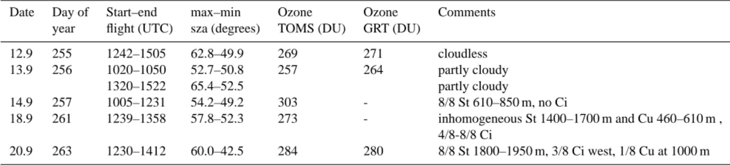
Table 3. Days analysed. Ozone values are from the ground-based GRT Brewer or the Earth Probe TOMS. Missing data are indicated by a -.
St=stratus, Cu=cumulus, Ci=cirrus. Cloud cover is given in oktas. In the table 3/8 Ci west is 3 oktas of cirrus located in the western part of the sky and 1/8 at Cu 1000 m indicates 1 okta of Cumulus clouds above 1000 m.
Date Day of Start–end max–min Ozone Ozone Comments year flight (UTC) sza (degrees) TOMS (DU) GRT (DU)
12.9 255 1242–1505 62.8–49.9 269 271 cloudless 13.9 256 1020–1050 52.7–50.8 257 264 partly cloudy 1320–1522 65.4–52.5 partly cloudy 14.9 257 1005–1231 54.2–49.2 303 - 8/8 St 610–850 m, no Ci 18.9 261 1239–1358 57.8–52.3 273 - inhomogeneous St 1400–1700 m and Cu 460–610 m , 4/8-8/8 Ci 20.9 263 1230–1412 60.0–42.5 284 280 8/8 St 1800–1950 m, 3/8 Ci west, 1/8 Cu at 1000 m
the lower error margin for the lowest wavelengths. The ra-diative transfer equation is solved by the discrete ordinate algorithm developed by Stamnes et al. (1988). This algo-rithm has been modified to account for the spherical shape of the atmosphere using the pseudo-spherical approximation (Dahlback and Stamnes, 1991). The pseudo-spherical radia-tive transfer equation solver was run in 16-stream mode. The extraterrestrial spectrum was adopted from several sources. Between 280 and 407.8 nm, the Atlas 3 spectrum shifted to air wavelengths was used. Atlas 2 (Woods et al., 1996) was used between 407.8 and 419.9 nm. Above 419.9 nm, the so-lar spectrum in the MODTRAN 3.5 radiation model was used (Anderson et al., 1993). The uncertainty in the model simu-lations is for a given condition controlled by the uncertainties in the input parameters. The effect of uncertainties in input parameters on the accuracy of model simulations have been investigated by Schwander et al. (1997) and Weihs and Webb (1997). Here it is noted that the present model for irradiances agree with other models and measurements to within ±3–5% under well-defined cloudless conditions (Mayer et al., 1997; Kylling et al., 1998; Van Weele et al., 2000). Comparison between the model and the albedometer (ALB) have been re-ported by Wendisch and Mayer (2003) to be within ±10% for the downwelling irradiances. The model agrees with ground-based actinic flux measurements within ±6% (Bais et al., 2003), and airborne actinic flux measurements within ±5% for altitudes between 3000–12 000 m (Hofzumahaus et al., 2002).
4 Cloud optical depth
To quantify the effect of clouds on the actinic flux, a measure is needed of the cloud optical depth over the domain. From the surface irradiance measurements, the effective cloud op-tical depth was derived using the method of Stamnes et al. (1991). The effective cloud optical depth is determined by comparing the irradiance at a wavelength where absorption by ozone is negligible with model-generated irradiances for various cloud optical depths. It is assumed that the cloud
is vertically homogeneous and that the effective droplet ra-dius is 10 µm. By effective cloud optical depth is meant the optical depth that when used in the model best reproduces the measurements. Hence, the effective cloud optical depth includes both aerosol and cloud optical depths. Mostly due to northerly winds, both lidar and sunphotometers showed very low aerosol abundances throughout the campaign, with typical 500-nm aerosol optical depth values ranging between 0.05 and 0.15. Hence, it may be assumed that the estimated effective cloud optical depths are not significantly affected by aerosols. In addition to the cloud optical depth, the cloud transmittance is derived by taking the ratio of the measured irradiance to the cloudless modelled irradiance. Except for the GRT spectroradiometer, a wavelength region centered at 380 nm and weigthed with a triangular function with a band-pass of 5 nm was used to estimate the effective cloud optical depth and the cloud transmittance. For the GRT instrument, a wavelength region centered at 350 nm was used.
The derivation of a cloud optical depth by this method is based on a direct comparison between measured and mod-elled irradiances. Hence, absolute agreement between the measurements and simulations must be ensured. In Fig. 1 ex-amples are shown of measured and simulated spectra during cloudless conditions. The agreement between the measure-ments and the model simulations is within the uncertainties associated with the measurements and the simulations and is of the same magnitude as that reported earlier by Mayer et al. (1997); Kylling et al. (1998) and Van Weele et al. (2000) for similar conditions. Differences between the measurements and the simulations of ±5% gives uncertainties of around 10% in the derived cloud optical depth. The uncertainty is largest for optically thin clouds.
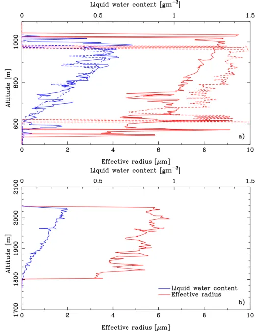
The cloud optical depths derived from the ground mea-surements were compared with in situ aircraft data for two days, days 257 and 263, when the sky was overcast. On both days the aircraft made several triangular patterns at con-stant altitudes above the ground stations and some profiles. Here attention is paid to the profile measurements. The liq-uid water content and the effective radius measured during
Fig. 1. Measured irradiance spectra, green lines, from the GRT instrument located at Briston, (a) and the NTN instrument at Aylsham, (b).
The spectra were recorded at 14:00 UTC on day 255. In blue is shown the uvspec model simulations of the spectra. The red lines are the model/measurement ratios. Note the different scales on the x-axes in a) and b).
the descent and ascent around 12:00 UTC on day 257 and the ascent on day 263 are shown in Fig. 2. Using the water cloud parameterization of Hu and Stamnes (1993), the pro-files on day 257 yield total cloud optical depths of about 30.3 for the descent and 19.7 for the ascent for a wavelength of 380 nm. The cloud on day 263 was thinner, with an optical depth of about 9.2. The differences in the optical depths on day 257 are mainly caused by differences in re between the
ascent (dashed line) and the descent (solid line). For short-wave radiation, the water cloud volume extinction coefficient
βextis directly related to the liquid water content, LW C, and
the droplet equivalent radius, re, (Stephens, 1978)
βext≈ 3 2 LW C re . (1)
Thus, for a constant LW C, a reduction in reby a factor of 2
will double the cloud optical depth. The in situ measured re
on day 263 is shown in Fig. 2 and varies over 4–9µm on day
257 and 3–6µm on day 263. It is generally increasing with altitude. The sensitivity of the water cloud optical depth to
re may be exemplified by noting that for the ascent on day
257 the in situ optical depth was 19.7 at 380 nm. Using the same LW C but constant reof 5, 7.5 and 10µm gives optical
depths of 34.6, 22.7 and 16.9, respectively.
The effective cloud optical depths measured from the sur-face are shown in the Figs. 3b and 3d. For day 257, the cloud optical depths deduced from the NTN and GRT instruments were both around 38 at 1200. At 1140 the NTN optical depth was 32. On day 263 the optical depths varied between 7 and 15 at the time the cloud profile was made (around 1300). These optical depths are larger than the optical depths de-rived from the in situ aircraft measurements. One possible reason for the discrepancy is cloud horizontal inhomogenity in the sense that the cloud optical depth was different at the locations of the aircraft and the ground stations.
Fig. 2. Liquid water content (blue lines) as measured by the PVM instrument and the effective radius (red lines) measured by the Fast-FSSP
instrument. In (a) the solid lines are from the descent and the dashed lines from the subsequent ascent on day 257. In (b) the data are from day 263. Note different scales on the y-axes.
For day 257, the profile was made about 0.1◦south of the
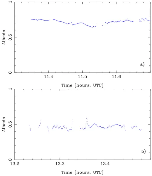
NTN site, and the wind was blowing from the north. On day 263, the profile was made slightly east of the Weybourne site. Thus, on both days cloud inhomogeneties may be part of the reason for the differences between the in situ and ground-based cloud optical depths. Just after the ascents on days 257 and 263, constant altitude legs were made above the clouds. The measured albedos derived from the Albedome-ter onboard the Partenavia, are shown in Fig. 4. The albedo appears to exhibit relatively small variations. However, the cloud optical depth of the underlying cloud may still vary
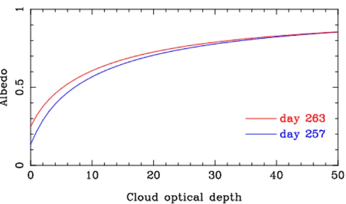
considerably. In Fig. 5 is shown model simulations of the albedo as a function of cloud optical depth at the two flight altitudes. The clouds vertical distribution were taken from Fig. 2 and the total optical depth scaled between 0 and 50. The solar zenith angles for the simulations were representa-tive for the flight conditions. For day 257, the albedo varied between 0.65 and 0.75. This corresponds to cloud optical depths between about 15 and 25. Similar numbers for day 263 are 0.4–0.5 for the albedo and 2–6 for the cloud op-tical depth. Thus, horizontal variations of the cloud may explain the differences between the in situ aircraft and the
Fig. 3. Downwelling actinic fluxes integrated between 380–400 nm at the ground, (a) day 257 and (c) day 263, as measured in Weybourne
(ATI, blue points), Beeston (GBM, red points), Briston (DEG, black points) and Aylsham (DED, green points). No data are available from the DED instrument on day 263. The black solid lines are cloudless model results for Weybourne, and the black dashed line is the solar zenith angle. In (b) and (d) are shown the effective cloud optical depths (squares) and the cloud transmittances (asterisks) for day 257, (b), and 263, (d). The black colours represent data from the GRT instrument, green the NTN instrument, and blue the ATI instrument. The black vertical lines indicate the interval in which the flights took place. Note different scales on y-axes of optical depth.
ground-based cloud optical depths. Nevertheless, the optical depths estimated from the ground measurements give a good indication of the horizontal variability over the domain and are used in the subsequent analysis.
5 Measurements versus simulations
Surface measurements were made continously in the period 12–29 September 2002. A number of flights were made dur-ing the same period. Here attention is paid to five days with clearly defined cloudless (1 day), overcast (2 days) and bro-ken clouds periods (2 days) (Table 3).
5.1 Cloudless situation
At the very first day of the main campaign, 12.9, day 255, the sky was partly cloudy until about 12:00 UTC. It then cleared up and the sky became cloudless. Also, VELIS indicated that no subvisible cirrus was present. During the cloudless condition, flights were made over the ground stations in a triangular pattern. In addition, the ground stations intensified their measurement schedules.
5.1.1 Ground data comparison
The time evolution of the downwelling actinic flux is shown in Fig. 6. The downwelling actinic flux is shown for a wave-length region where ozone absorbs, 305–320 nm (Fig. 6a) and a wavelength region where ozone does not absorb, 380– 400 nm (Fig. 6b). The different diurnal behaviour of the ac-tinic flux in these two wavelength regions is evident. It is caused by the larger direct contribution to the total actinic flux at larger wavelengths. In addition to the measurements, simulations of the cloudless actinic flux are shown as well. The dip in the modelled clear-sky actinic flux between 1500 and 16:30 UTC is caused by significant increases, from about 0.05 to about 0.2, in the aerosol optical depth. For the in-tegrated 380–400 nm wavelength range, the DED measure-ments are about 2–4% smaller, while the ATI measuremeasure-ments are 4–6% higher than the simulations. The GBM measure-ments are 0–2% lower than the simulations for the same range. For the integrated 305–320 nm range, ATI and GBM are 3–10% higher than the model simulation, and DED is 3–10% lower. These spectral differences are also visible in individual spectra, as shown in Fig. 7 for the ATI and DED instruments, together with uvspec model simulations. The spectral resolution is higher for the spectrum from the ATI
Fig. 4. Albedo for the 380–400 nm interval measured at constant flights altitudes of about 2830 m, day 257 (a), and 2349 m, day 263 (b).
The albedo is derived from irradiance measurements onboard the Partenavia. Data points where the pitch of the aircraft was larger than 5◦ or the roll was larger than 1◦have been excluded.
instrument. This is due to the spectral width of the slit func-tion, which is 0.5 and 2.2 nm at FWHM for the ATI and DED instruments, respectively.
The measurement-model differences are of the same mag-nitude to those reported by Fr¨uh et al. (2003) for 2π ground-based measurements of the actinic flux and to those reported by Hofzumahaus et al. (2002). In the latter, the 4π spec-tral actinic flux measured between 120 m to 13 000 m by an aircraft-mounted spectroradiometer was compared to the same radiative transfer model used here. Considering the un-certainties in both the measurements and the simulations, it is concluded that the simulations and the measurements agree within the uncertainties. Furthermore, the overall agreement between the measurements and the model simulations of the actinic flux is similar to that for the irradiances presented in Fig. 1.
The spectral actinic flux is about a factor 2 larger than the simultaneously measured irradiances shown in Fig. 1. This is in agreement with the theoretical predicitions for these so-lar zenith angles and atmospheric conditions of (e.g., Kylling et al., 2003b, in their Figs. 1 and 2 and Eq. 7). It is noted that no simple relationship exists between the irradiance and the actinic flux as such a relationship depends on various atmo-spheric parameters, all of which are generally not available (Ruggaber et al., 1993; Van Weele, Arellano and Kuik, 1995; Kylling et al., 2003b).
5.1.2 Aircraft data comparison
The flights made during the cloudless period went up to an altitude of about 2000 m. The ascent starting at 13.6068 and ending at 13.8767 UTC was selected for further analysis. The
Fig. 5. Albedo as a function of cloud optical depth for days 257
(blue line) and 263 (red line). The albedo for day 257 (263) is cal-culated for a flight altitude of 2835 (2349) m and a solar zenith angle of 49.3◦(54.8◦).
solar zenith angle varied between 53.3◦and 54.8◦during the ascent. This variation in solar zenith angle caused less than 2% (6%) variations in the surface downwelling actinic flux in the UVA (UVB). This time slot is in the middle of the cloudless period, hence the data are minimally effected by possible clouds on the horizon.
In Fig. 8 is shown examples of the measured downwelling and upwelling actinic fluxes at some altitudes. Also shown are model simulations and model/measurement ratios. The downwelling measured and simulated actinic fluxes for all al-titudes agree similarly to the measured and simulated irradi-ances shown in Fig. 1. The model overestimates by about 3– 4% below 320 nm and underestimates by 5–7% above about 350 nm. This is within the combined model and measure-ment uncertainties. The latter is estimated to ±8% in the UV range (305–400 nm) and ±5% in the visible (400–700 nm) (J¨akel et al., 2005). For the upwelling spectra, the disagree-ment between the model and measuredisagree-ments is larger. For the 58 m altitude upwelling spectrum, the overall agreement is reasonable. Part of the structure seen may be caused by un-accounted wavelength shifts. All ground and aircraft spec-tra, except the upwelling aircraft specspec-tra, have been wave-length shift corrected with the SHICRIVM algorithm (Slaper et al., 1995). The model overestimates the upwelling spec-trum at 1961 m significantly below about 380 nm. There is also a similar trend for the spectrum at 58 m . Causes for the differences may be attributed to several reasons. One is the non-perfect angular response of the input optics. This gives crosstalk between the upper and lower hemisphere. For low-albedo and low-altitude conditions, the contributions from the upper hemisphere to the lower hemisphere signal may be considerable (see Hofzumahaus et al., 2002, Fig. 6). The angular response correction depends on altitude, wavelength, surface albedo and solar zenith angle. In addition, clouds and aerosol will affect the correction. Angular correction fac-tors as a function of wavelength, altitude, cloud, and surface
albedo have been calculated using the discrete ordinate algo-rithm developed by Stamnes et al. (1988). A thorough dis-cussion of the correction factors has been presented by J¨akel et al. (2005). The measurements have been corrected for the non-perfect angular response using these factors, how-ever, an ideal correction implies complete knowledge about the sky radiance, which is not generally available. Also, the upwelling fluxes are rather sensitive to the albedo of the un-derlying surface. Uncertainties in the surface albedo esti-mate causes large changes in the upwelling radiation, espe-cially for low altitudes and longer wavelengths. However, since the agreement was reasonable at 58 m and the albedo is small for the conditions here, the albedo is not a likely cause for the differences at 1961 m. Furthermore, uncertain-ties in the aerosol optical depth, single-scattering albedo and asymmetry factor may affect the model results the most for the upwelling actinic flux at 1961 m. The operational pitch and roll angles range of the stabilization system is ±6◦.
Dur-ing the ascent the acceleration of the aircraft meant that this range in periods was exceeded. Data outside the operational range was excluded from the analysis. Nevertheless, part of the ascent and descent data may be influenced by air-craft movements although the magnitude is assumed to be small. While the differences between the model and mea-surements are larger for the upwelling than the downwelling actinic flux, it is noted that the magnitude of the upwelling actinic flux is much smaller than the downwelling actinic flux for a cloudless sky and a small albedo. Hence, the contribu-tion to the 4π actinic flux is rather small from the upwelling part. Note that the FWHM of the DFD and DFU instruments is about 2.5 nm. Hence, the spectra shown in Fig. 8 have similar spectral structure to those shown for the DED instru-ment in Fig. 7. In Fig. 9 vertical profiles are shown of the measured and simulated up- and downwelling actinic fluxes integrated over the 380–400 nm and 305–320 nm wavelength intervals. The differences between the measured and simu-lated actinic fluxes reflects the spectral differences discussed above and shown in Fig. 8. Both the down- and upwelling actinic fluxes increase with altitude for both wavelength in-tervals presented. The increase is largest for the upwelling actinic fluxes because as the altitude increase, the amount of atmosphere below the aircraft increase, thereby causing an increase of upscattered radiation due to Rayleigh scatter-ing. The wavelength dependence of the Rayleigh scattering cross section also causes the increase in the upwelling actinic fluxes to be largest for short wavelengths. Similarily, the in-crease with altitude of the downwelling actinic flux is largest for the shortest wavelengths.
Except for the upwelling actinic flux, the model and the measurement agree within their uncertainties for the cloud-less case. Furthermore, the measurements made at the dif-ferent ground stations agree within their uncertainties. With this in the mind, attention is turned to overcast situations.
Fig. 6. Downwelling actinic fluxes at the ground as measured in Weybourne (ATI, blue points), Beeston (GBM, red points), and Aylsham
(DED, green points), integrated between 305–320 (a) and 380–400 nm, (b). The black solid lines are cloudless model results for Weybourne. All data are from day 255. The black vertical lines indicate the interval in which the flights took place. The black dashed lines are the solar zenith angles.
5.2 Overcast
Two days, 14th and 20th of September (days 257 and 263), were considered as “homogeneous” overcast cases. In par-ticular, 14 September was a “clean” situation with no cirrus above the stratocumulus cloud layer (Table 3).
5.2.1 Ground data comparison
In Fig. 3 the time evolution of the measured actinic flux on the ground is shown during the flights on these days. Also, the effective cloud optical depth as deduced from the surface irradiance measurements is shown. Compared to the cloud-less situation, the actinic flux is reduced by about 75% (50%) on day 257 (263). The variability in the actinic flux during the flight hours indicates that the cloud was not horizontally homogeneous, and the downwelling actinic flux at times
ex-hibited differences of about 40% between the stations. These variations are also seen in the cloud optical depth and trans-mittance in Figs. 3b and 3d. During the flight, the wind was from the north and relatively strong.
5.2.2 Aircraft data comparison
In Fig. 10 the measured and simulated actinic fluxes are shown as a function of altitude for the ascents (blue) and de-scent (red) on days 257 and 263. The black lines are model simulations of the measurements. The effect of the clouds on the actinic flux is similar on both days. Above the cloud the actinic flux is enhanced, a maximum is observed just below the cloud top in the downwelling actinic flux, and below the cloud the actinic flux is reduced compared to the cloudless situation. The variability seen at about 2900 m for the de-scent (red points) and 1500 m for the ade-scent (blue points) day
Fig. 7. Measured actinic flux spectrum (a), green line, from the ATI instrument located at Weybourne. The spectrum was recorded at
14:00 UTC on day 255. In blue is shown the uvspec model simulation of the spectrum. The red solid line is the model/measurement ratio.
(b) Similar to (a) but for the DED instrument at Aylsham.
257, are due to the aircraft spending some time at these alti-tudes, thus viewing different parts of the clouds. These vari-ations thus indicate cloud horizontal inhomogeneities and their effect of about 11% on the downwelling and total ac-tinic fluxes for these measurements.
The above-cloud enhancement depends on the optical thickness of the cloud (see Fig. 9 of Van Weele and Duynkerke, 1993). The optical depth for the descent on day 257 was 30.3 and reduced to 19.7 for the ascent. A thicker cloud has a higher albedo, thus the above cloud actinic flux is higher for the descent, red points and dashed line in Fig. 10, compared to the ascent, blue points and solid line. Corre-spondingly, the optically thicker cloud transmits less radia-tion, resulting in lower below-cloud radiation than the opti-cally thinner cloud.
Just below the cloud top, theory predicts a maximum in the actinic flux. The maximum has theoretically been de-scribed by Madronich (1987) and Van Weele and Duynkerke (1993). The magnitude of the maximum is largest for small solar zenith angles and decreases as the solar zenith angles increases (de Roode et al., 2001, and Fig. 11). Also, the magnitude of the maximum increases with increasing cloud optical depth, while the geometric extent decreases with in-creasing cloud optical depth. The effect disappears for large solar zenith angles. The maximum occurs at optical depths were the direct beam is still significant and the diffuse radi-ation is becoming appreciable. It is noted that for the solar zenith angles encountered during days 257 and 263 (Table 3), the calculations shown in Fig. 11 indicate that the maximum might be seen in the downwelling actinic flux measurement.
Fig. 8. Downwelling actinic flux (a) (green line) at an altitude of 1961 m as measured by the DFD spectroradiometer on day 255 at
1353 (hhmm) and 12.9 s. (b) The upwelling actinic flux (green line) measured by the DFU spectroradiometer on day 255 at an alti-tude of 1961 m, dashed lines, (58 m, solid lines) at 1350 and 44 s (1336 and 4.9 s). Model simulations are shown as blue lines and the model/measurements ratios are shown in red.
Fig. 9. Downwelling (blue points) and upwelling (red points) actinic fluxes as a function of altitude integrated between 305–320 nm (a) and
Fig. 10. Measured downwelling, (a) and (c), and total, (b) and (d) (downwelling plus upwelling) actinic fluxes integrated between 380–
400 nm as a function of altitude for days 257 (a) and (b), and 263, (c) and (d). The blue points are from the ascents and the red points from the descent. Descent data for day 263 are not available as the descent was made outside the grid box under investigation. The dashed and solid lines represent simulations of the ascent and descents respectively. The dotted black lines are cloudless model calculations and the horizontal green lines indicate the top and bottom of the cloud layers.
Inspection of the measurements and the model simulations of the downwelling actinic flux, Fig. 10a and c, reveals a maximum for both days. It is noted that for the ascent on day 257, the maximum is not observed. This may be due to the lack of data in the topmost part of the cloud or cloud top inhomogeneties. No enhancement is seen in the total actinic flux. This is in agreement with the model predic-tions shown in Fig. 11 where a maximum is observed in the downwelling actinic flux for a solar zenith angle of 40◦, but not in the total actinic flux. Similar enhancements around cloud top have been observed in tethered-balloon measure-ments by de Roode et al. (2001) and Vil`a–Guerau de Arel-lano et al. (1994). Below the maximum the actinic flux decreases monotonically with decreasing altitude until cloud bottom. Below the cloud the actinic flux varies little with altitude. This is typically for the effect of clouds over sur-faces with a low albedo. Over high-albedo sursur-faces such as snow, the behaviour is significantly different (de Roode et al., 2001).
The overall agreement in Fig. 10 between the model simu-lations and the measurements is good. The simusimu-lations cap-ture the main feacap-tures of the measurements. However, some differences are evident, especially below the cloud bottom
where the model is consistently larger than the measurements for day 257 and smaller then the measurements for day 263. As shown in Fig. 4, the clouds were not homogeneous, which clearly affected the radiation measurements. The relative dif-ferences in the transmittance between the stations were larger on day 263 compared to day 257 (see Fig. 3). This further in-dicates cloud horizontal inhomogeneities, which may explain the larger below-cloud differences for day 263 compared to day 257. The model simulations are 1-D and hence do not account for any horizontal variability.
Compared to a cloudless atmosphere, the cloud on day 257 increases the downwelling actinic flux by about 30% above the cloud and reduces it by about 65% below. Similar num-bers for the total actinic flux are about 100% and 55%, re-spectively. The cloud on day 263 is thinner, hence more ra-diation penetrates the cloud and less is scattered back. The total (downwelling) flux is increased by about 60% (20%) above the cloud and reduced by about 55% (55%) below the cloud. These number for the total actinic flux are in agree-ment with those reported by e.g. Vil`a–Guerau de Arellano et al. (1994) and Shetter and M¨uller (1999).
Fig. 11. Modelled downwelling, (a), and total (downwelling plus upwelling), (b), actinic fluxes for 360 nm as a function of altitude for
various solar zenith angles.
5.3 Broken clouds
The above discussed cases may be considered “simple” 1-D upon visual inspection although closer analysis reveal possi-ble 3-D effects. More complex cases include broken clouds, multi-layer clouds and combinations of these. On day 256, “cloud bands” oriented west-east covered 4 oktas (4/8) over land. A snapshot of the cloud bands is provided in Fig. 12. There was no cirrus on that day. Day 261 was a rather com-plex situation with quite inhomogeneous cumulus/stratus be-tween 500 and 1900 m and 4/8 to 8/8 cirrus bebe-tween 11 and 14 km. The cloud inhomogeneity was clearly visible from below (see Fig. 12). Two flights were made on day 256. Data from the second and longest flight are analysed here together with data from the flight on day 261.
5.3.1 Ground data comparison
In Fig. 13 the downwelling actinic flux measured on the ground on these two days during the flights is shown. Also shown are the effective cloud optical depths and transmit-tances as deduced from the ground measurements. On day 256, the cloud bands were only present inland. This is seen in Fig. 13, as the measurements by the ATI and GBM in-struments on the coast are representative of cloudless condi-tions. The inland measurements by the DED instrument vary rapidly as the cloud bands pass over the measurement site. Occassionally the measurements are larger than the cloud-less model simulations, shown as a solid black line. This indicates the combined effect of scattering off cloud sides and a visible solar disk (Mims and Frederick, 1994; Nack and Green, 1974). The variations seen in the actinic flux of the DED instrument are also evident in the transmittance and
13.09.2002 1420
18.09.2002 1334
Fig. 12. All-sky pictures taken at Briston on day 256 at 1420 (top) and day 261 at 1334 (bottom).
cloud optical depths deduced from the inland GRT and NTN instruments. Note, however, that the time resolution of these instruments are lower than for the DED instrument. Both episodes of cloud gaps and cloud bands are readily identified in Fig. 13. The steps in the cloudless model results, black solid lines, are due to changes in the aerosol optical depth deduced from VELIS.
On the ground fewer variations are seen at the individual stations on day 261 (see Fig. 13). However, the variations between the stations are of the same magnitude as the varia-tions at Aylsham, DED, on day 256. Thus, while the sky ap-peared to be more homogeneous on day 261 compared to day 256, Fig. 12, the cloud inhomogeneties caused considerable variations over the area covered by the ground stations. This
Fig. 13. Downwelling actinic fluxes, (a) and (c) at the ground as measured in Weybourne (ATI, blue points), Beeston (GBM, red points),
Briston (DEG, black points) and Aylsham (DED, green points). The black solid lines are cloudless model results for Weybourne and the black dashed lines are the solar zenith angles. The effective cloud optical depth (squares) and the cloud transmittance (asterisks) are shown for days 256 (b) and 261, (d). The black colour represents data from the GRT instrument, green the NTN instrument, and blue the ATI instrument. The black vertical lines indicate the interval in which the flights took place.
is also evident in the albedo measurements shown in Fig. 14. Most of time the aircraft is above the clouds. The parts within the clouds are readily identified by large and spurious varia-tions in the albedo. These are during the ascents and descents at the beginning and end of both flights and around 1400 for the flight on day 256. For both days, the large variations in the albedo measured while the aircraft was above the clouds reflect the horizontal inhomogeneties of the clouds. For day 256, the minimum albedo is close to the cloudless albedo, while the maximum albedo reflects that the clouds were not optically thick on this day. On the other hand, the clouds on day 261 were thicker, with smaller and fewer gaps, thus producing the higher minimum and maximum albedos. 5.3.2 Aircraft data comparison
In order to simulate the measurements, vertical profiles of the liquid water content and effective droplet radius are required. As the clouds were inhomogeneous, it was not possible to select data from a single cloud penetration as done above for days 257 and 263. Instead, all liquid water content data from the PVM and all effective radius data from the Fast-FSSP were plotted as a function of altitude, Fig. 15. For the cloud band, day 256, it was assumed that the cloud was ver-tically homogeneous with a liquid water content of 0.5 gm3
and re=5.5 µm. Cloud bottom was at 900 m and cloud top
at 930 m. With the Hu and Stamnes (1993) parameterization, this resulted in a cloud optical depth of 4.3 at 380 nm. The optical depths derived from the ground measurements var-ied between 10 and 16 when clouds were overhead, Fig. 13. As discussed earlier, this difference may be caused by cloud horizontal inhomogeneties.
For day 261 the clouds had a larger vertical extent. A near-adiabatic liquid water profile was assumed and values between the maximum and minimum measured liquid wa-ter contents adopted. The re was assumed to increase with
altitude, Fig. 15. This resulted in an optical depth of 31.7 at 380 nm. The inland, ground-deduced optical depths var-ied between 20 and 25, which, again considering horizontal variations, is consistent with the cloud built from the PVM and Fast-FSSP measurements.
In Fig. 16, the total and downwelling actinic fluxes mea-sured by the Partenavia on days 256 and 261 are shown as a function of altitude. Also shown are model simulations for cloudless and cloudy conditions. For the cloudy sim-ulations, the cloud properties shown in Fig. 15 were used. As mentioned earlier, day 256 was characterised by cloud bands oriented west-east. Thus, from the ground, it was ei-ther cloudy or the sun could be seen. The flight on day 256
Fig. 14. Albedo at 380 nm measured during the flights on day 256, (a), and day 261, (b). The albedo is derived from irradiance measurements
onboard the Partenavia. The black solid lines show the altitude of the aircraft. Data points where the pitch of the aircraft was larger than 5◦ or the roll was larger than 1◦have been excluded.
lasted for about 2.5 h. During this time period the solar zenith angle increased from about 52◦to 65◦. This changed the ac-tinic fluxes by about 30% below the cloud and about 25% for the cloudless conditions. The variability seen in the actinic fluxes of about ±10% when the aircraft was at constant alti-tude above the clouds, reflects the changes in the cloud cover underneath. See, for example, the horizontally oriented data points at about 1600, 2300 and 2800 m in Fig. 16a and b. The ground measurements on day 256 of the downwelling actinic flux varies between 6 and 19 W/m2, Fig. 13. This is in agreement with the below-cloud aircraft measurements (see Fig. 16). Above the cloud, the aircraft measurements are 0–150% larger than the cloudless ground measurements.
For day 261, the picture is more complicated due to the horizontal and vertical variations of the cloud cover. The cloud simulations obviously have the cloud bottom placed
a little too high. The ground measurements varied between 3 and 16 W/m2(see Fig. 13). The same variability is not seen in the aircraft data. However, this is caused by the fact that only one ascent and descent was made on that day. Thus, the aircraft data may not be fully representative for the whole area in its full vertical and horizontal extent.
As can be seen in Fig. 16, the measurements lie between the cloudless, Fclear, and cloudy, Fcloudy, 1-D model
simu-lations. Thus, for this situation a simple cloud fraction, Cf,
approximation
F = CfFcloudy+(1 − Cf)Fclear (2)
might yield representative values for the total actinic flux, F , provided that the vertical extent of the cloud and its optical properties were known, and that a realistic value of Cf is
Fig. 15. Liquid water content, (a), as measured by the PVM instrument and the effective radius, (b), measured by the Fast-FSSP instrument.
Red dots are data from day 256 and blue dots data from day 261. The solid lines are the input used for the model simulations.
0.7 (blue) were used for Cf. The above cloud actinic flux
is reasonably well captured by any of these cloud fractions. However, below the cloud the actinic flux is either repre-sented by cloudless or overcast calculations. Thus the cloud fraction approximation appears to only capture part of the picture for this situation. For day 261, values of 0.5 (green), 0.6 (red) and 0.7 (blue) were used for Cf. The overall best
agreement both above and below the cloud is obtained with a value of 0.6, although the below-cloud actinic flux is slightly overestimated. The best agreement below the cloud is ob-tained for Cf=0.8 (not shown). However a value of 0.8
over-estimates the actinic flux above the cloud. Thus, the cloud fraction approach appears to be too simple to describe both the above-cloud enhancement and the below-cloud reduction by a single number. It must also be noted that during such
inhomogeneous and changing conditions, it is not feasible to sample a larger area with aircraft. Thus, the measured data may not be fully representative for the area under investiga-tion.
Based on the images shown in Fig. 12, the cloud amounts are estimated to 4 oktas on day 256 and between 7 and 8 oktas for day 261. The relationship between cloud amount as estimated by a surface observer and the earthview (ver-tical) cloud amount needed in radiative transfer models has been discussed by Henderson-Sellers and McGuffie (1990) and references therein. For mid-range cloud amounts, the two views are comparable. This agrees with the findings here that a Cf=0.5 gives a reasonable representation above the
cloud for day 256. For large cloud amounts, surface observa-tions tend to overestimate cloud amount as compared to the
Fig. 16. Downwelling, (a) and (c), and total, (b) and (d), actinic fluxes integrated between 380–400 nm for the entire flights on day 256, (a)
and (b), and day 261, (c) and (d), as a function of altitude. The solid lines are model simulations including the model clouds from Fig. 15 with different cloud fractions. For day 256, black is Cf=1.0; green Cf=0.3; red Cf=0.5, and blue Cf=0.7. Similarily for day 261, black
is Cf=1.0; green Cf=0.5; red Cf=0.6, and blue Cf=0.7. The dashed lines are cloudless model simulations. For all lines, the rightmost
(leftmost) lines are for the smallest (largest) solar zenith angles encountered during the flights, see Fig. 13. The horizontal green lines indicate the top and bottom of the cloud layers.
earthview cloud amount. This is also found here, as a value of Cf=0.9, or about 7 oktas, overestimates the actinic flux
by about 16% above the cloud and underestimates the actinic flux by about 33% below the cloud, compared to Cf=0.6.
Thus, while all-sky images are useful to document the mea-surement conditions and in the selection of interesting cases, direct use of cloud amounts deduced from these images must be used with care in models.
6 Conclusions
As part of the INSPECTRO project, an extensive campaign to study the influence of clouds on the spectral actinic flux in the lower troposphere was carried out in East Anglia, Eng-land, September 2002. The spectral actinic flux, the irra-diance and aerosol and cloud properties were measured by aircraft and four ground stations.
Data from cloudless, broken cloud and overcast situa-tions were selected for analysis. A detailed radiative transfer model was used to simulate and interpret the measurements. The following findings were made.
– For cloudless conditions, the measurements of the
to-tal and downwelling actinic flux were reproduced by the radiative transfer model within the measurement and model uncertainties of about ±10%.
– Under cloudless conditions the upwelling actinic flux
contributed between 5 to 30% to the total actinic flux depending on wavelength and altitude. Above 300 nm the measured and simulated downwelling actinic fluxes agreed within ±10%. For shorter wavelengths the dif-ferences were larger.
– For cloud conditions visually characterised as
horizon-tally homogeneous, the downwelling actinic flux at the surface at times varied by up to 40% between sta-tions for the rather small experimental area of about 12×12 km2. Simultaneously, the above-cloud varia-tions in the downwelling and total actinic fluxes were about 11% over the area.
– For overcast situations, 1-D radiative transfer
calcu-lations reproduced the overall behaviour of the ac-tinic flux measured by the aircraft. Especially, the
above-cloud enhancement and below-cloud reductions are well characterized.
– The above-cloud enhancement increases with
increas-ing optical depth. Similarily, the below-cloud reduction increases with increasing optical depth.
– Just below the cloud top, the downwelling actinic flux
has a maximum, which is seen in both the measure-ments and the model results.
– For broken-cloud situations, the cloud fraction approach
captures some of the changes in the actinic flux. How-ever, no single value for the cloud fraction is able to reproduce the measured above-cloud enhancement and below-cloud reductions for the analysed situations. Thus, we conclude that for the cases studied here, cloud-less and overcast single-layered clouds may be satisfacto-rily simulated by 1-D radiative transfer models. The rel-atively simple broken-cloud cases investigated indicate that for these cloud situations and more-complex cases 3-D cor-rections must be applied. What these corcor-rections look like is an outstanding research question.
As part of the INSPECTRO project, a second campaign was conducted in May 2004 in southern Germany covering a larger, about 50×50-km2, area to further elucidate the impact of clouds on the actinic flux.
Acknowledgements. This research was funded by contract
EVK2-CT-2001-00130 from the European Commission. Funding by the German Science Foundation (DFG) and the German Research Ministry (BMBF) are acknowledged. Part of this research was performed while one of the authors (M. W.) held a National Re-search Council ReRe-search Associateship Award at the NASA Ames Research Center. As usual the enviscope GmbH company and the pilot of the Partenavia, Bernd Schumacher, did an excellent job in preparing and conducting the measurements with the Partenavia.
Edited by: A. Hofzumahaus
References
Anderson, G., Clough, S., Kneizys, F., Chetwynd, J., and Shet-tle, E.: AFGL atmospheric constituent profiles (0–120 km), Tech. Rep. AFGL-TR-86-0110, Air Force Geophys. Lab., Hanscom Air Force Base, Bedford, Mass., 1986.
Anderson, G. P., Chetwynd, J. H., Theriault, J.-M., Acharya, P. K., Berk, A., Robertson, D. C., Kneizys, F. X., Hoke, M. L., Abreu, L. W., and Shettle, E. P.: MODTRAN2: Suitability for re-mote sensing, in: Atmospheric Propagation and Rere-mote Sens-ing, SPIE Conf. Ser., vol. 1968, edited by: Kohnle, A. and Miller, W. B., pp. 514–525, Soc. of Photo–Optical–Instrum. Eng., Bellingham, Wash., 1993.
Bais, A. F., Madronich, S., R., J. C. S., Hall, J., Mayer, B., van Weele, M., G., J. L. J., Calvert, Cantrell, C. A., Shetter, R. E., Hofzumahaus, A., Koepke, P., Monks, P. S., Frost, G., McKen-zie, R., Krotkov, N., Kylling, A., Swartz, W. H., Lloyd, S.,
Pfister, G., Martin, T. J., Roeth, E.-P., Griffioen, E., Ruggaber, A., Krol, M., Kraus, A., Edwards, G. D., Mueller, M., Lefer, B. L., Johnston, P., Schwander, H., Flittner, D., Gardiner, B. G., Barrick, J., and Schmitt, R.: International Photolysis Frequency Measurement and Model Intercomparison (IPMMI): Spectral ac-tinic solar flux measurements and modeling, J. Geophys. Res., 108, doi:10.1029/2002JD002 891, 2003.
Barnaba, F. and Gobbi, G.: Modeling the aerosol extinction versus backscatter relationship in a mixed maritime-continental atmo-sphere: Lidar application and validation, J. Atm. Ocean Technol., 21, 428–442, 2004.
Bass, A. M. and Paur, R. J., The ultraviolet cross–section of ozone, I, The measurements, in: Atmospheric Ozone: Proceedings of the Quadrennial Ozone Symposium, edited by: Zerefos, C. S. and Ghazi, A., pp. 601–606, D. Reidel, Norwell, Mass., 1985. Brasseur, A.-L., Ramaroson, R., Delannoy, A., Skamarock, W., and
Barth, M.: Three-dimensional calculation of photolysis frequen-cies in the presence of clouds and impact on photochemistry, J. Atmos. Chem., 41, 211–237, 2002.
Cahalan, R. F., Ridgway, W., Wiscombe, W. J., Gollmer, S., and Harshvardhan: Independent pixel and Monte Carlo estimates of stratocumulus albedo, J. Atmos. Sci., 51, 3776–3790, 1994. Chambers, L. H., Wielicki, B. A., and Evans, K. F.: Accuracy of
the independent pixel approximation for satellite estimates of oceanic boundary layer cloud optical depth, J. Geophys. Res., 102, 1779–1794, 1997.
Crawford, J., Shetter, R., Lefer, B., Cantrell, C., Junkermann, W., Madronich, S., and Calvert, J.: Cloud impacts on UV spectral ac-tinic flux observed during the International photolysis frequency measurement and model intercomparison (IPMMI), J. Geophys. Res., 108, doi:10.1029/2002JD002 731, 2003.
Dahlback, A. and Stamnes, K.: A new spherical model for com-puting the radiation field available for photolysis and heating at twilight, Planet. Space Sci., 39, 671–683, 1991.
de Roode, S. R., Duynkerke, P. G., Boot, W., and der Hage, J. C. H. V.: Surface and tethered-balloon observations of actinic flux: effects of arctic stratus, surface albedo, and solar zenith angle, J. Geophys. Res., 106, 27 497–27 507, 2001.
Evans, K. F., The spherical harmonics discrete ordinate method for three–dimensional atmospheric radiative transfer, J. Atmos. Sci., 55, 429–446, 1998.
Fr¨uh, B., Trautmann, T., Wendisch, M., and Keil, A.: Comparison of observed and simulated NO2photodissociation frequencies in a cloudless atmosphere and continental boundary layer clouds, J. Geophys. Res., 105, 9843–9857, 2000.
Fr¨uh, B., Eckstein, E., Trautmann, T., Wendisch, M., Fiebig, M., and Feister, U.: Ground-based measured and calculated spectra of actinic flux density and downward UV irradiance in cloudless conditions and their sensitivity to aeosol microphysical proper-ties, J. Geophys. Res., 108, doi:10.1029/2002JD002 933, 2003. Gobbi, G. P., Barnaba, F., Giorgi, R., and Santacasa, A.:
Altitude-resolved properties of a Saharan dust event over the Mediter-ranean, Atmos. Environ., 34, 5119–5127, 2000.
Gobbi, G. P., Barnaba, F., and Ammannato, L.: The vertical distri-bution of aerosols, Saharan dust and cirrus clouds at Rome (Italy) in the year 2001, Atmos. Chem. Phys., 4, 351–359, 2004,
Henderson-Sellers, A. and McGuffie, K.: Are cloud amounts esti-mated from satellite sensors and conventional surface-based ob-servations related?, Int. J. Remote Sensing, 11, 543–550, 1990. Hofzumahaus, A., Kraus, A., Kylling, A., and Zerefos, C.: Solar
actinic radiation (280–420 nm) in the cloud-free troposphere be-tween ground and 12 km altitude: Measurements and model re-sults, J. Geophys. Res., 107, 10.1029/2001JD900 142, 2002. Hu, Y. X. and Stamnes, K.: An accurate parameterization of the
radiative properties of water clouds suitable for use in climate models, J. Climate, 6, 728–742, 1993.
J¨akel, E., Wendisch, M., Kniffka, A., and Trautmann, T.: A new airborne system for fast measurements of up- and downwelling spectral actinic flux densities, Appl. Opt., 44, 434–444, 2005. Junkermann, W.: Measurements of the J(O1D) actinic flux within
and above stratiform clouds and above snow surfaces, Geophys. Res. Lett., 21, 793–796, 1994.
Kelley, P., Dickerson, R. R., Luke, W. T., and Kok, G. L.: Rate of NO2photolysis from the surface to 7.6 km altitude in clear-sky and clouds, Geophys. Res. Lett., 22, 2621–2624, 1995.
Kylling, A., Bais, A. F., Blumthaler, M., Schreder, J., Zerefos, C. S., and Kosmidis, E.: The effect of aerosols on solar UV irradiances during the Photochemical Activity and Solar Ultraviolet Radia-tion campaign, J. Geophys. Res., 103, 26 051–26 060, 1998. Kylling, A., Danielsen, T., Blumthaler, M., Schreder, J., and
Johnsen, B.: Twilight tropospheric and stratospheric photodisso-ciation rates derived from balloon borne radiation measurements, Atmos. Chem. Phys., 3, 377–385, 2003a,
SRef-ID: 1680-7324/acp/2003-3-377.
Kylling, A., Webb, A. R., Bais, A. F., Blumthaler, M., Scmitt, R., Thiel, S., Kazantzidis, A., Kift, R., Misslbeck, M., Schallhart, B., Schreder, J., C.Topaloglou, Kazadzis, S., and Rimmer, J.: Actinic flux determination from measurements of irradiance, J. Geophys. Res., 108, doi:10.1029/2002JD003, 236, 2003b. Lantz, K. O., Shetter, R. E., Cantrell, C. A., Flocke, S. J., Calvert,
J. G., and Madronich, S.: Theoretical, actinometric, and radio-metric determinations of the photolysis rate coefficient of NO2 during the Mauna Loa Observatory Photochemistry Experiment 2, J. Geophys. Res., 101, 14 613–14 629, 1996.
Los, A., van Weele, M., and Duynkerke, P. G.: Actinic fluxes in broken cloud fields, J. Geophys. Res., 102, 4257–4266, 1997. Madronich, S.: Photodissociation in the atmosphere 1. Actinic flux
and the effects of ground reflections and clouds, J. Geophys. Res., 92, 9740–9752, 1987.
Matthijsen, J, Suhre, K., Rosset, R., Eisele, F. L., Mauldin III, R. L., and Tanner, D. J.: Photodissociation and UV radiative transfer in a cloudy atmosphere: Modeling and measurements, J. Geophys. Res., 103, 16 665–16 676, 1998.
Mayer, B., Seckmeyer, G., and Kylling, A.: Systematic long–term comparison of spectral UV measurements and UVSPEC model-ing results, J. Geophys. Res., 102, 8755–8767, 1997.
Mayer, B., and Kylling, A.: Technical note: The libRadtran soft-ware package for radiative transfer calculations – description and examples of use, Atmos. Chem. Phys., 5, 1855–1877, 2005,
SRef-ID: 1680-7324/acp/2005-5-1855.
Mims, F. M. I. and Frederick, J. E.: Cumulus clouds and UV-B, Nature, 371, 291, 1994.
Monks, P. S., Rickard, A. R., Hall, S. L., and Richards, N. A. D., Attenuation of spectral actinic flux and photolysis frequencies at the surface through homogenous cloud fields, J. Geophys. Res.,
109, doi:10.1029/2003JD004 076, 2004.
Nack, M. L. and Green, A. E. S.: Influence of clouds, haze, and smog on the middle ultraviolet reaching the ground, Appl. Opt., 13, 2405–2415, 1974.
Nicolet, M.: On the molecular scattering in the terrestrial atmo-sphere: An empirical formula for its calculation in the homo-sphere, Planet. Space Sci., 32, 1467–1468, 1984.
Ramanathan, V., Cess, R. D., Harrison, E. F., Minnis, P., Barkstrom, B. R., Ahmad, E., and Hartmann, D.: Cloud–radiative forcing and climate: results from the Earth radiation budget experiment, Science, 243, 57–63, 1989.
Ruggaber, A., Forkel, R., and Dlugi, R.: Spectral actinic flux and its ratio to spectral irradiance by radiation transfer calculations, J. Geophys. Res., 98, 1151–1162, 1993.
Schwander, H., Koepke, P., and Ruggaber, A.: Uncertainties in modeled UV irradiances due to limited accuracy and availabil-ity of input data, J. Geophys. Res., 102, 9419–9429, 1997. Shetter, R. E. and M¨uller, M.: Photolysis frequency measurements
using actinic flux spectroradiometry during the PEM-Tropics mission: instrumentation description and some results, J. Geo-phys. Res., 104, 5647–5661, 1999.
Slaper, H., Reinen, H. A. J. M., Blumthaler, M., Huber, M., and Kuik, F.: Comparing ground-level spectrally resolved solar UV measurements using various instruments: A technique resolving effects of wavelengths shift and slit width, Geophys. Res. Lett., 22, 2721–2724, 1995.
Stamnes, K., Tsay, S.-C., Wiscombe, W., and Jayaweera, K.: Nu-merically stable algorithm for discrete-ordinate-method radiative transfer in multiple scattering and emitting layered media, Appl. Opt., 27, 2502–2509, 1988.
Stamnes, K., Slusser, J., and Bowen, M.: Derivation of total ozone abundance and cloud effects from spectral irradiance measure-ments, Appl. Opt., 30, 4418–4426, 1991.
Stephens, G. L.: Radiation profiles in extended water clouds. II: Parameterization schemes, J. Atmos. Sci., 35, 2123–2132, 1978. Stephens, G. L. and Tsay, S.-C.: On the cloud absorption anomaly,
Q. J. R. Meteorol. Soc., 116, 671–704, 1990.
Thompson, A. M.: The effect of clouds on photolysis rates and ozone formation in the unpolluted troposphere, J. Geophys. Res., 89, 1341–1349, 1984.
Trautmann, T., Podgorny, I., Landgraf, J., and Crutzen, P. J.: Ac-tinic fluxes and photodissociation coefficients in cloud fields em-bedded in realistic atmospheres, J. Geophys. Res., 104, 30 173– 30 192, 1999.
Van Weele, M., and Duynkerke, P. G.: Effect of Clouds on the Pho-todissociation of NO2: observations and modelling, J. Atmos. Chem., 16, 231–255, 1993.
Van Weele, M. de Arellano, J. V.-G., and Kuik, F.: Combined mea-surements of UV-A actinic flux, UV-A irradiance and global radi-ation in relradi-ation to photodissociradi-ation rates, Tellus, 47B, 353–364, 1995.
Van Weele, M., Martin, T. J., Blumthaler, M., Brogniez, C., den On-ter, P. N., Engelsen, O., Lenoble, J., Mayer, B., PfisOn-ter, G., Rug-gaber, A., Walravens, B., Weihs, P., Gardiner, P. G., Gillotay, D., Haferl, D., Kylling, A., Seckmeyer, G., and Wauben, W. M. F.: From model intercomparison towards benchmark UV spectra for six real atmospheric cases, J. Geophys. Res., 105, 4916–4925, 2000.