DOI 10.1007/s10531-008-9541-y O R I G I N A L P A P E R
Scenario-based assessment of future land use change
on butter
Xy species distributions
Michael Lütolf · Janine Bolliger · Felix Kienast · Antoine Guisan
Received: 10 April 2008 / Accepted: 17 November 2008 / Published online: 6 December 2008
© Springer Science+Business Media B.V. 2008
Abstract Species distribution models (SDMs) are increasingly used to predict environ-mentally induced range shifts of habitats of plant and animal species. Consequently SDMs are valuable tools for scientiWcally based conservation decisions. The aims of this paper are (1) to identify important drivers of butterXy species persistence or extinction, and (2) to analyse the responses of endangered butterXy species of dry grasslands and wetlands to likely future landscape changes in Switzerland. Future land use was represented by four scenarios describing: (1) ongoing land use changes as observed at the end of the last cen-tury; (2) a liberalisation of the agricultural markets; (3) a slightly lowered agricultural pro-duction; and (4) a strongly lowered agricultural production. Two model approaches have been applied. The Wrst (logistic regression with principal components) explains what envi-ronmental variables have signiWcant impact on species presence (and absence). The second (predictive SDM) is used to project species distribution under current and likely future land uses. The results of the explanatory analyses reveal that four principal components related to urbanisation, abandonment of open land and intensive agricultural practices as well as two climate parameters are primary drivers of species occurrence (decline). The scenario analyses show that lowered agricultural production is likely to favour dry grassland species due to an increase of non-intensively used land, open canopy forests, and overgrown areas. In the liberalisation scenario dry grassland species show a decrease in abundance due to a strong increase of forested patches. Wetland butterXy species would decrease under all four scenarios as their habitats become overgrown.
Keywords Agricultural change · Explanatory model · GLM · PCA · Predictive model · Scenario · Species distribution model (SDM)
M. Lütolf · J. Bolliger · F. Kienast (&)
Swiss Federal Research Institute WSL, Zuercherstrasse 111, CH-8903 Birmensdorf, Switzerland e-mail: [email protected]
M. Lütolf
e-mail: [email protected] M. Lütolf · A. Guisan
Introduction
Land use changes entailing species habitat destruction have been identiWed as major causes of species extinctions (Ehrlich and Ehrlich 1981; Wilson 1988; Dirzo and Raven 2003). Expansion of settlements and infrastructure as well as changes in agricultural practices have been among the most prominent driving forces of these changes in Western Europe over the last 50–60 years (Ewald 1978; PWster 1995; Chamberlain et al. 2000; Bätzing 2003). The ongoing changes in agricultural practices can be characterised either by agricul-tural intensiWcations or land abandonment processes. Agricultural intensiWcation is mostly observed on fertile soils with moderate slopes in regions with well developed infrastruc-ture, whereas land abandonment is rather characteristic of poor soils, heavily sculptured terrain, and remote areas. Both intensiWcation and land abandonment have initiated an accelerated decrease in habitat diversity and species richness (Suarez-Seoane et al. 2002; Bolliger et al. 2007 #324; Dullinger et al. 2003; Vickery et al. 2004; Lindborg et al. 2005). Even though species richness might increase after land abandonment due to an increase in the heterogeneity and diversity of the tree layer (Söderström et al. 2001), it has been claimed that, in the longer term, a continued aVorestation will Wnally result in negative eVects (Laiolo et al. 2004; Brennan and Kuvlesky 2005).
Hence, to enable a sustainable management of the biological resources in the sense of the Rio Convention on Biological Diversity (http://www.biodiv.org) species distribution models (SDMs) (Guisan and Zimmermann 2000) relating species presence/absence data to physical environmental characteristics are a valuable tool to study species reactions under changing environments (Bolliger et al. 2000; Stefanescu et al. 2004; Guisan and Thuiller 2005). Such models have been increasingly used to support decisions in nature conserva-tion planning (Glenz et al. 2001; Barbosa et al. 2003; Peterson and Robins 2003). For that purpose, scenarios for future landscapes have often been created to provide descriptions of plausible developments (Tress and Tress 2003; Bolliger et al. 2007). Scenarios do not claim to predict or forecast the most realistic outcome, but rather to oVer a way to think about alternative directions of change (Tress and Tress 2003).
In this study we analyse the potential impacts of four scenarios of agricultural change in Switzerland on the distribution of two groups of butterXy species, predominately inhabiting dry grasslands or wetlands, respectively. The habitats of both species groups have experienced quantitative and qualitative declines since the 1950s. With the upcom-ing agricultural intensiWcation, such non-intensively used areas have been preferably transformed by drainage and/or fertilisation into more productive areas under cultivation (Eggenberg et al. 2001). Hence, their conservation has become a major concern of local, regional, and national environmental policies. The four scenarios of land use change describe: (1) a continuation of the land use/land cover changes as observed between 1985 and 1997 (“business as usual” scenario); (2) a liberalisation of the current agricultural markets (“liberalisation” scenario); (3) a trend towards a slightly less intensive agricul-ture (scenario of a “moderately lower agricultural production”); and (4) a trend towards an even less productive agriculture (scenario of a “strongly lower agricultural produc-tion”) (Bolliger et al. 2007). For a detailed description of the scenarios see paragraph “characteristics of the scenarios”.
In particular, we address the following two research questions: (1) which factors are the best to explain the current species distribution and might strongly inXuence future species occurrence? (2) how will butterXy species distribution change under diVerent scenarios of agricultural change? The Wrst question is investigated using an explanatory model, whereas the second question is analysed with a predictive SDM.
Materials and methods
Study area
Switzerland is situated in Western Europe and covers an area of 41,293 km2. Based on the distribution of plant and animal species, the country was divided into six major biogeo-graphic regions (Fig.1; Gonseth et al. 2001). The climate is generally temperate humid. However, it is locally strongly inXuenced by the mountainous topography and thus climate ranges from oceanic with high annual rainfalls (Northern Alps, Jura Mountains) to intra-alpine dry and continental (Central Alps). The Southern Alps show an insubrian climate, characterised by mild and dry winters but warm and humid summers. According to climate and topography, agriculturally productive areas are mainly situated on the Plateau, at an altitude of 360–600 m a.s.l. In the Jura Mountains (highest elevation at 1,600 m a.s.l.) and the Alps (upto 4,600 m a.s.l.) dairy farming prevails.
Politically, Switzerland is divided into 26 cantons, further subdivided into the smallest political entities, the communes. In the present study we use data that are aggregated to the spatial extent of the 2,836 communes present in 2003. The average area of a commune is 1,410 ha (standard deviation 2,294 ha). The median is 700 ha, indicating that most com-munes are smaller than the average.
Scenarios of land use change
Characteristics of the scenarios
The scenarios used in this study rely on two drivers of land use change: (1) the societal role of agricultural production; and (2) the public support for conservation issues (Bolliger
et al. 2007). The ‘business as usual’ scenario (BAU) assumes that structural changes observed between the 1980s and 1990s (BFS 1979/85, 1992/97) will continue in the same way until the year 2020. Even though the main product of the farms will be food produc-tion, the income will substantially depend on the adopted agri-environmental scheme. The liberalisation scenario (LIB) assumes that the agricultural markets are no longer subsidized with e.g. product payments or direct payments bound to agri-environmental schemes. As a result, only farms located in highly productive regions, e.g. on the Plateau, would be proWtable and able to generate food at world-market prices. Farming in the mountains would be largely abandoned. This in turn would favour spontaneous reforestation on fallow land. The two remaining scenarios assume a moderately (LAP1) and a strongly (LAP2) lowered agricultural production under a liberalised agricultural market. Farmers are assumed to adopt agri-environmental schemes, intensify production of organic and other niche products and land use would be optimized (with subsidies) for conservation purposes.
Land use data and spatial implementation of the scenarios
The Swiss land use statistics provide a description of 74 diVerent land use classes for two time periods, i.e. 1979–1985 and 1992–1997 (BFS 1979/85, 1992/97). The data set covers the whole study area. The original point data were derived from aerial photographs and fur-ther assigned to a grid with a cell size of 100 £ 100 m (1 ha).
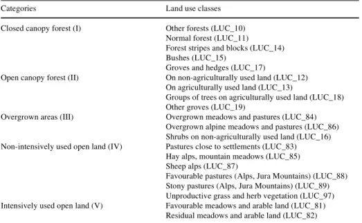
The scenarios considered Wve aggregated categories of land use classes representing: (I) closed canopy forest; (II) open canopy forest; (III) overgrown areas; (IV) non-intensively used open land; and (V) intensively used open land. The remaining land use classes were left unchanged in the scenarios (Table1, for details see Rutherford et al. 2008). This aggre-gation was conducted to capture the broad changes that allowed ecologically meaningful inferences about successional processes (Gillian Rutherford, personal communication, 2006).
The spatial implementation of the scenarios relied on: (1) transition frequencies; and (2) spatially explicit transition probabilities (Bolliger et al. 2007). Transition frequencies de W-ned the fraction of a land use category to change into another one. For the ‘business as usual’ scenario transition frequencies were derived from changes in land use between 1985 and 1997. For the three remaining scenarios these were derived using qualitative socio-eco-nomic judgement. Thereby, the transition frequencies for the strongly lowered agricultural production (LAP) scenario were generally twice as high as for the moderate scenario (Bolliger et al. 2007). Transition probabilities indicated the chance of every individual grid cell to change its land use category. Probabilities were calculated from GLMs relating land use change between 1985 and 1997 to abiotic variables like topography, slope or aspect (Rutherford et al. 2008).
Scenario-based land use changes of the Wve categories were spatially implemented by randomly converting cells into the new land use categories within areas of highest probabil-ity of change. Thereby, cells were converted until the scenario-based transition frequencies were accomplished. Changes in land use were analysed for the six biogeographic regions represented in Fig.1.
Species data
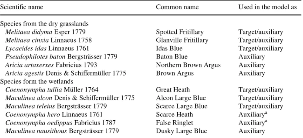
We selected six butterXy species as biotic dependent variables due to species sensitivity to changes in land use (Table2). They were referred to as ‘target’ species and either repre-sented species inhabiting predominantly dry grasslands or wetlands. The aggregation of the
species was conducted to enlarge the number of species presence data used in the models. The Spotted Fritillary (Melitaea didyma), the Glanville Fritillary (Melitaea cinxia), and the Idas Blue (Lycaeides idas) are still relatively widely distributed in the Central and Southern Alps, whereas in the northern part of the country they have shown severe declines due to losses of their preferred habitats (Gonseth 1987). All three species preferably inhabit dry grasslands where they live on of a large variety of host plants. The altitudinal distribution ranges from the lowlands upto 1,600–2,400 m a.s.l. The preferred habitats of the Great Heath (Coenonympha tullia), the Scarce Large Blue (Maculinea teleius), and the Alcon Large Blue (Maculinea alcon) are typically wetlands like fens or non-intensively cultivated bog areas. During the 1990s they were most frequently observed in the Eastern part of the Plateau and the Northern Alps as well as in the Western parts of the Jura Mountains, the Plateau, and the Northern Alps. The species appear from the low elevations upto 1,200– 1,400 m a.s.l. Drainage and intensive agriculture are mentioned among the most prominent factors that have caused strong declines in species populations (Gonseth 1987).
Data of butterXy species presences were provided by the Swiss Centre for Faunal Car-tography (CSCF) and originated from natural history collections (NHC, Graham et al. 2004). We chose the communal level regarding it as the appropriate scale for this study since: (1) the species data were most representative as aggregations on the communal level and (2) changes in land use derived from comparisons of the Swiss land use statistics should only be interpreted for broader scales and not for single cells of 1 ha due to sam-pling errors resulting from the applied spot sample method (BFS 1997).
Because valid species absences were missing in the natural history collection data that would have served to Wt the species models we introduced pseudo-absences (Zaniewski et al. 2002; Engler et al. 2004) based on (1) historical distribution data and (2) presences of
Table 1 Aggregation of the 74 land use classes (LUC) of the Swiss land use statistics 1992/1997 (BFS 1992/97) into Wve categories (I–V) (according to Rutherford et al. 2008)
The remaining 54 classes (describing settlements, infrastructure, areas for fruit-growing, rock, glaciers, lakes, and wider rivers) were left unchanged
Categories Land use classes
Closed canopy forest (I) Other forests (LUC_10) Normal forest (LUC_11)
Forest stripes and blocks (LUC_14) Bushes (LUC_15)
Groves and hedges (LUC_17)
Open canopy forest (II) On non-agriculturally used land (LUC_12) On agriculturally used land (LUC_13)
Groups of trees on agriculturally used land (LUC_18) Other groves (LUC_19)
Overgrown areas (III) Overgrown meadows and pastures (LUC_84) Overgrown alpine meadows and pastures (LUC_86) Shrubs on non-agriculturally used land (LUC_16) Non-intensively used open land (IV) Pastures close to settlements (LUC_83)
Hay alps, mountain meadows (LUC_85) Sheep alps (LUC_87)
Favourable pastures (Alps, Jura Mountains) (LUC_88) Stony pastures (Alps, Jura Mountains) (LUC_89) Unproductive grass and herb vegetation (LUC_97) Intensively used open land (V) Favourable meadows and arable land (LUC_81)
species showing similar habitat requirements as the modelled species (further referred to as ‘auxiliary species’) (Lütolf et al. 2006). This procedure was preferred to a random sam-pling of absence communes since it was shown that considering historical species distribu-tion data result in higher model performances (Lütolf et al. 2006). Hence, for either the dry grassland or the wetland species group, we assigned another three butterXy species that were referred to as “auxiliary” species (Table1). The selection of “pseudo-absence” com-munes involved the following steps: (1) from the total of 2,836 comcom-munes present in Switzerland in 2003 we excluded the communes where target species were recorded between 1991 and 2000 (since these communes were used as species presence data in the model; see beneath). (2) From the remaining communes we further excluded communes with recent presence records (1991–2000) of the auxiliary species. As auxiliary species can share the same habitats as the target species it might be highly probable that also target spe-cies could occur in these communes, even though they were not collected. (3) We further excluded historical presence records (1901–1990) of the modelled and the auxiliary species. Step (3) was necessary to exclude any commune that could perhaps provide habitat for the species due to historical reasons, but was not visited between 1991 and 2000. Using this selection approach we obtained pools of pseudo-absences with 2,163 (dry grassland species group) and 2,568 (wetland species group) potential pseudo-absence communes.
For both species groups, the presence data of the three target species from the period 1991–2000 were pooled and multiple records of a given commune deleted. The resulting 172 (dry grassland species) and 78 (wetland species) communes were used as species pres-ence data in the model.
Environmental predictors
We described the landscape structure of a commune using the percentages of the 20 land use classes (Table1). We complemented the initial set of land use predictors with degree-days above 3.0°C and the water budget in July. Degree-days consider time and temperature by only integrating the positive diVerence between the daily mean tempera-ture and the threshold temperatempera-ture of 3.0°C over a year. The water budget was calculated
Table 2 ButterXy species selected as model species (target) or as species used to deWne pseudo-absences
(auxiliary) by considering historical presences between 1951 and 1990
aSpecies assumed to be extinct in Switzerland nowadays
ScientiWc name Common name Used in the model as
Species from the dry grasslands
Melitaea didyma Esper 1779 Spotted Fritillary Target/auxiliary
Melitaea cinxia Linnaeus 1758 Glanville Fritillary Target/auxiliary
Lycaeides idas Linnaeus 1761 Idas Blue Target/auxiliary
Pseudophilotes baton Bergsträsser 1779 Baton Blue Auxiliary
Aricia artaxerxes Fabricius 1793 Northern Brown Argus Auxiliary
Aricia agestis Denis & SchiVermüller 1775 Brown Argus Auxiliary Species form the wetlands
Coenonympha tullia Müller 1764 Great Heath Target/auxiliary
Maculinea alcon Denis & SchiVermüller 1775 Alcon Large Blue Target/auxiliary
Maculinea teleius Bergsträsser 1779 Scarce Large Blue Target/auxiliary
Coenonympha hero Linnaeus 1761 Scarce Heath Auxiliarya
Coenonympha oedippus Fabricius 1787 False Ringlet Auxiliarya
as the diVerence between the precipitation and the potential evapotranspiration. Both predictors were available as grid maps with a spatial resolution of 25 m. The maps were calculated using monthly averages of climate data from meteorological stations through-out the study area of the period 1961–2000. The spatial interpolation between the sta-tions was achieved using SPLINE funcsta-tions (see Zimmermann and Kienast 1999). We aggregated the climate data for every commune and derived the minimum values that were used as predictors in the models (degree-days: DEGD30MIN; July water budget: WBJULMIN). The minimum values were preferred over mean and maximum values since (a) several studies show positive correlations between physiologically limiting fac-tors (minimum facfac-tors) and butterXy occurrence (Crozier 2003; Menzel et al. 2006), and (b) our own calculations showed that less residual deviance remained unexplained when minimum values were applied.
Statistical analyses
Two model approaches were applied. The Wrst approach (explanatory model) aims at explaining which environmental factors are signiWcantly correlated with observed species distributions. The second approach (predictive SDM) is used to predict butterXy species distribution for future land use scenarios.
Explanatory models
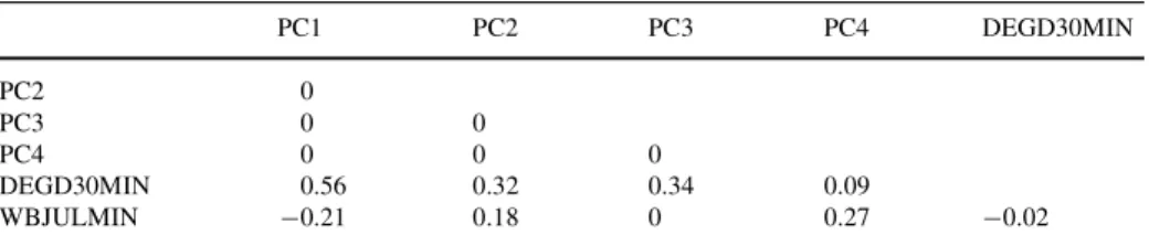
For both butterXy species groups, we investigated which land use types of the land use sta-tistics 1992/97 (BFS 1992/97) explained current species distributions. We Wrst performed a principal component analysis (PCA) on the covariance matrix of the 21 land use vari-ables to obtain uncorrelated factors representing land use characteristics. The components were interpreted according to the loadings obtained. We selected the Wrst four principal components as land use predictors for further analyses according to the ecological inter-pretability and explained variance achieved (see section on results). Together with the cli-matic variables used in the predictive models (minimum degree-day sum above 3°C and minimum July water budget) these two principal components composed the predictor dataset for the explanatory models. The relatively high correlation of the Wrst principal component with the degree-day predictor (DEGD30MIN) was further reduced by loga-rithmically transforming the degree-day values. The correlations between predictors are shown in Table3.
We conducted model calibration, parameter selection, and model evaluation according to the procedures described for the predictive models.
Table 3 Correlation coeYcients for the explanatory model
PC1-4, principal components 1–4; DEGD30MIN, logarithm of the minimum degree-days with a threshold temperature of 3.0°C; WBJULMIN, minimum July water budget
PC1 PC2 PC3 PC4 DEGD30MIN PC2 0 PC3 0 0 PC4 0 0 0 DEGD30MIN 0.56 0.32 0.34 0.09 WBJULMIN ¡0.21 0.18 0 0.27 ¡0.02
Fitting the predictive models
We applied standard generalised linear models (GLM, McCullagh and Nelder 1989) with a binomial family and a logistic link function to relate species data to the environmental pre-dictors. The arc-sinus transformation of the square root of the percentage of the land use predictors was used to normalise these explanatory variables (Mosteller and Tukey 1977). GLMs have widely and successfully been used to model species potential distributions based on presence-absence data (Guisan et al. 1998, 2002; Manel et al. 1999; Zimmermann and Kienast 1999; Bolliger et al. 2000; Bailey et al. 2002; Luoto et al. 2002; Guisan and Hofer 2003). We did not account for multicollinearity between the 23 parameters, as delet-ing one or more highly correlated variables of our dataset might have reduced the eVective-ness of our model as a predictive tool (Leahy 2000). Multicollinearity is a problem when the goal is as presented below—explanation, since it increases the standard error of the sampling distribution of the coeYcients of highly collinear variables (Leahy 2000).
Generalised linear models were Wtted within the R statistical software package (R 1.9.1—a language and environment, © 2004). The number of pseudo-absences matched the number of presences, so that a prevalence of 0.5 was ensured. The selection of pseudo-absences from the initial pools was conducted randomly. To account for the variation in the results of this random selection we Wtted 1,000 model runs with diVerent sets of pseudo-absences (Engler et al. 2004). For each Wtted model, the Wnal set of predictors was obtained by a stepwise backward selection based on Akaike’s Information Criterion (AIC). The Wt of every model run was expressed by the percentage of deviance explained by the respective GLM. Additionally, the adjusted percent deviance explained (see Guisan and Zimmermann 2000) that takes into account the number of observations and parameters used to build the model was computed.
Evaluating the predictive models
Model evaluation aims to assess the accuracy of model predictions. We used the calibration data set to evaluate the models by applying a leave-one-out jack-knife procedure (Manly 1997; Guisan and Zimmermann 2000; Jaberg and Guisan 2001). A new GLM was Wtted on a dataset reduced by a single observation at a time. This procedure was repeated until every observation of the dataset was left out once. At each run, the Wtted model was used to pre-dict the response for the excluded observation. The obtained prepre-dictions were reclassiWed to presence–absence (1/0) for all threshold values between 0.05 and 0.95 by increment of 0.05. Then, confusion matrices with the observed presence–absence information were gen-erated (see Fielding and Bell 1997). The Kappa statistic (Cohen 1960; see Fielding and Bell 1997) was calculated for every confusion matrix and the maximum Kappa value (max Kappa) was assigned to the model (Guisan and Hofer 2003; Engler et al. 2004). Since the evaluation metrics derived from confusion matrices can be sensitive to prevalence (propor-tion of presences, see Fielding and Bell 1997; Manel et al. 2001), we addi(propor-tionally used the threshold independent area under the receiver operating characteristic (ROC) curve (AUC Fielding and Bell 1997). The AUC takes values between 0.5 and 1.0, where a value of 0.5 indicates a chance performance and a value of 1.0 represents a model that perfectly sepa-rates presences and absences. Values between 0 and 0.5 can also be obtained sometimes and indicate a performance worse than obtained by chance.
Since for both species groups 1,000 model runs were performed, the evaluation statistics were calculated for each run. An overall species model performance and standard error was obtained by averaging the evaluation results of the 1,000 runs.
Assessing species occurrence under likely future land use
We modelled the probabilities of occurrence for both butterXy species groups under current (LU97) as well as future land use (scenarios BAU, LIB, LAP1 and LAP2). The climatic variables were kept constant. For each scenario, probabilities of occurrence from 1,000 model runs were averaged for each biogeographic region (Jura Mountains, Plateau, North-ern Alps, SouthNorth-ern Alps, WestNorth-ern and EastNorth-ern Central Alps). As described above, the initial SDM was Wtted with the detailed land use classes listed in Table1 (twenty land use classes and two climate classes). For the scenario SDMs, however, only lumped predictor classes were available. In order to use the initial SDM calibration (with detailed land use classes) for the scenario runs and to generate consistent results we applied the following rules: (1) since we do not know the future composition of detailed land use classes within the lumped classes we assumed a constant ratio for all scenarios. In other words, if e.g. category I (closed canopy forest) has a composition of 50% “other forests”, 20% “bushes” and 30% “forest stripes and blocks” (Table1) this composition will be kept constant and no addi-tional land use classes will be “generated” within category I. Thus the scenario-driven changes in the subclasses are dependent on the changes in the lumped classes only. (2) The scenarios assume that the absolute amount of pixels in the Wve lumped classes remains con-stant over time, or, in other words, there is no pixel that changes from one of the Wve clas-ses to urban or bare plots and vice versa. (3) To calculate the probabilities of occurrence of each species under scenario conditions we applied the GLMs calibrated for the detailed land use classes.
Results
Explanatory model
Results of the PCA
The Wrst four principal components explained 87% of the variation in the land use data (Table4). The Wrst component explained 46% of the variation and represented a gradient from intensively cultivated meadows and arable land to non-intensively used pastures in the Alps and Jura Mountains. The second component accounted for another 21% of varia-tion and was mainly a gradient from areas covered by settlements, infrastructure or other agriculturally unproductive land uses (e.g. glaciers or rocks) to closed canopy forests. The third component explained 12% of the variation. Here, the gradient extended from non-intensively used agricultural areas in the form of favourable pastures of the Alps and Jura Mountains to closed forested area. The fourth component explained 7% of the variation and mainly represented a gradient towards less intensively used arable land, meadows, and pas-tures in the vicinity of settlements where Weld sizes become smaller and slopes steeper.
Factors inXuencing species presence
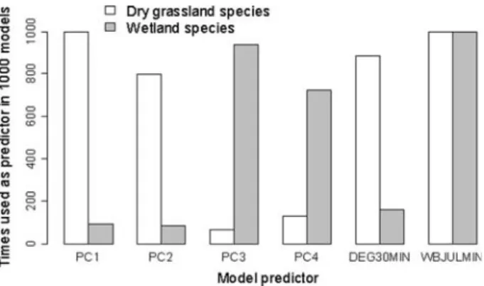
The number of times a predictor was used to Wt the explanatory models (1,000 model runs in total were conducted) is shown in Fig.2. Thereby, after the AIC-based backward selec-tion procedure the principal components 1 (PC1) and 2 (PC2) were almost exclusively retained in the models of the dry grassland butterXy species. Contrary, the Wnal models of
the wetland butterXy species were mainly Wtted with the principal components 3 (PC3) and 4 (PC4) that together explained ca. 20% of the variance in the PCA. The minimum water budget for July was selected as climatic predictor in both species models, whereas the min-imum degree-day sum above 3°C was mainly used to Wt the model of the dry grassland spe-cies. Averages and standard deviations of the model coeYcients are given in Table5a.
The explanatory model for the dry grassland species group explained 45% of the devi-ance, whereas the model for the wetland species group explained 25% (Table5b). Model accuracy for the Wrst group was similar to the predictive model (Kappa, 0.68; AUC, 0.91) indicating a very good agreement between predicted and observed presences and pseudo-absences according to the ranking of Monserud and Leemans (1992). Fair agreement resulted for the wetland species group (Kappa, 0.52; AUC, 0.82).
Scenarios of land use change
Compared to the landscape in 1997, the ‘BAU’ scenario revealed marginal changes in area for all categories (closed and open canopy forest, overgrown areas, non-intensively and intensively used open land) across the biogeographic regions (cf. Fig.1). The main land use changes resulting from this scenario can be summarised as follows: (1) closed canopy for-est areas slightly increased in all biogeographic regions, (2) non-intensively used open land increased in the Northern, the Eastern Central as well as the Southern Alps, and (3) inten-sively used open land increased on the Plateau and in the Jura Mountains.
Table 4 Results of the PCA for the Wrst four principal components
LUC; according to Table1. Loadings between ¡0.1 and 0.1 are not displayed and therefore, land use catego-ries 10, 18, 19, and 84 are omitted
Component Proportion of variance (%) Cumulative proportion (%)
(a) The total variance explained by the Wrst four principal components
PC1 46.4 46.4
PC2 21.3 67.7
PC3 12.3 80.0
PC4 7.4 87.4
Variable PC1 PC2 PC3 PC4
(b) Loadings of the land use classes
LUC_11 ¡0.175 0.631 0.501 ¡0.285 LUC_14 0.118 LUC_15 ¡0.133 ¡0.103 ¡0.149 LUC_17 0.146 LUC_12 ¡0.149 ¡0.129 LUC_13 ¡0.111 LUC_86 ¡0.114 ¡0.138 LUC_16 ¡0.161 ¡0.128 LUC_83 0.110 0.420 LUC_85 ¡0.155 LUC_87 ¡0.155 LUC_88 ¡0.340 0.139 ¡0.600 0.146 LUC_89 ¡0.102 ¡0.140 LUC_97 ¡0.226 ¡0.109 ¡0.209 ¡0.161 LUC_81 0.803 ¡0.313 ¡0.250 LUC_82 0.110 0.724 LUC_OTHER ¡0.728 0.366
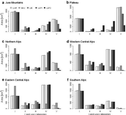
The main eVect of the LIB scenario was a general increase in wooded area (Fig.3). Hence, in all Alpine biogeographic regions, strong increases in closed and open canopy forest and overgrown areas (except in the Southern Alps) were visible. On the Plateau the LIB scenario did not aVect the current forested area. In hilly and mountainous regions the proportion of non-intensively used open land was lowered at the expense of forested area, whereas on the Plateau non-intensively used open land was converted into intensively used open land.
The scenarios assuming LAP did not aVect the area covered by closed canopy forests (Fig.3). For the moderate scenario (LAP1) the major changes compared with the state in 1992/1997 were: (1) increases in open canopy forest and overgrown areas in all biogeo-graphic regions; (2) increases in non-intensively used open land in the Jura Mountains, the Northern Alps, and on the Plateau (decreases resulted because more non-intensively
Fig. 2 Number of times the predictors for the explanatory models remained in the Wnal models after an
AIC-based backward selection. PC1-4, principal components 1–4; DEGD30MIN, logarithm of the minimum de-gree-days with a threshold temperature of 3.0°C; WBJULMIN, minimum water budget in July
Table 5 Explanatory model
Dry grassland species: M. didyma, M. cinxia, and L. idas. Wetland species: C. tullia, M. alcon, and M. teleius. PC1-4, principal components 1–4; DEGD30MIN, logarithm of the minimum degree-days with a threshold temperature of 3.0°C; WBJULMIN, minimum water budget in July
Predictor Dry grassland species model, n = 1,000 Mean § SD
Wetland species model, n = 1,000 Mean § SD
(a) Model coeYcients
PC1 ¡3.70 § 0.53 ¡0.51 § 1.30 PC2 1.57 § 0.37 1.26 § 1.14 PC3 0.13 § 1.65 ¡2.62 § 0.71 PC4 ¡2.04 § 0.68 3.43 § 0.96 DEGD30MIN ¡0.85 § 0.37 0.09 § 1.14 WBJULMIN ¡0.04 § 0.01 0.03 § 0.01
Species group Model Wts, n = 1,000 Model evaluation, n = 1,000
D2: mean § SD Adjusted D2: mean § SD Kappa AUC (b) Model Wts and evaluation measures of 1,000 GLMs conducted for each species group
Dry grassland species 0.45 § 0.03 0.45 § 0.03 0.68 0.91
used open land turned into overgrown areas than was gained by the conversion of inten-sively used open land); and (3) mostly strong decreases in the area of inteninten-sively used open land in the whole country (Fig.3). In the scenario describing strongly lowered agri-cultural production (LAP2) (1) the intensively used open land continued to decrease and (2) the areas of open canopy forest, overgrown areas, and non-intensively used open land in the Jura Mountains, on the Plateau, and in the Northern Alps increased even more (Fig.3).
Predictive distribution model
Performance of the GLMs
The results of the model Wtting displayed in Table6 show that 52% (dry grassland species model) and 48% (wetland species model) of the total deviance were explained by the envi-ronmental predictors. Model accuracies measured with the Kappa statistics revealed a fair to good agreement between observed and predicted species presences and absences
Fig. 3 Areas covered by the land use categories I–V (I closed canopy forest, II open canopy forest, III
over-grown area, IV non-intensively used open land, V intensively used open land) under the current land use (LU97) and the four land use change scenarios (BAU business as usual, LIB liberalisation, LAP1 moderately lowered agricultural production, LAP2 strongly lowered agricultural production)
(Monserud and Leemans 1992). This agreement was also conWrmed by the threshold inde-pendent assessment using the AUC value (Hosmer and Lemeshow 2000).
Patterns of species distribution under the scenarios
The probability of occurrence of dry grassland species was only little aVected under the ‘BAU’ scenario (Fig.4a). In the Jura Mountains and on the Plateau, this scenario slightly favoured species probability of occurrence, whereas in all other biogeographic regions the species probability of occurrence was slightly reduced. The LIB scenario favoured the dry grasslands species in the Jura Mountains and the Northern and Eastern Central Alps (Fig.4a). On the Plateau and in the Western Central Alps no changes in the probability of occurrence were predicted, whereas in the Southern Alps the probability was again reduced. Species probability of occurrence was mainly aVected by the scenarios describing LAP in the Jura Mountains and on the Plateau (Fig.4a). Compared to the current land use (LU97) these two scenarios that favoured open canopy forest, overgrown areas and non-intensively used open land achieved probabilities of occurrence between 60 and 80%. However, a moderate lowering of the agricultural production (LAP1) revealed lower prob-abilities of occurrence compared to the current land use (LU97) in the remaining four regions. Instead, a stronger lowering (LAP2) achieved higher probabilities compared to the LAP1 scenario, but only resulted in higher probabilities compared to the current land use in the Northern Alps (Fig.4a).
Compared to the dry grassland species the wetland butterXy species were not favoured by scenarios describing LAP (Fig.4b). Except for the Southern Alps, where no species was found in the 1990s, the probabilities of species occurrence were lower than under the current land use (LU97) and even decreased from MFB1 to MFB2. In the Jura Mountains and on the Plateau the LIB scenario revealed a slight increase in the probabilities, whereas in the other biogeographic regions probabilities were lower than under the current land use.
Discussion
Factors aVecting species distribution
Our results revealed that dry grassland species distribution was mainly negatively corre-lated to a gradient from non-intensive to intensive land use (Wrst principal component) and positively correlated to a gradient from more urbanised areas to closed forests (second prin-cipal component). The distribution of wetland species was negatively correlated with a gra-dient from non-intensively to intensively used open land to closed forest (third principal
Table 6 Predictive model
Model Wts and evaluation measures of 1,000 GLMs conducted for each species group (dry grassland species:
M. didyma, M. cinxia, and L. idas. Wetland species: C. tullia, M. alcon, and M. teleius)
Species group Model Wts, n = 1,000 Model evaluation, n = 1,000
D2, mean § SD Adjusted D2, mean § SD Kappa AUC Dry grassland species 0.52 § 0.04 0.51 § 0.04 0.69 0.93
component) and positively correlated with a gradient describing an increasingly less inten-sive land use in the vicinity of settlements (fourth principal component). Thus, our results are in accordance with the Wndings of Stefanescu et al. (2004) who found that human pres-sure and modern-day agricultural practices negatively aVected Mediterranean butterXy diversity. Even though it has been shown that butterXy species presence also depends on habitat quantity (Luoto et al. 2002), this could not be conWrmed from our results since the principal components only represent land use qualities.
Climatically, wetland species showed a clear positive correlation to increasing July water budgets, whereas dry grassland species preferred areas where dryer conditions pre-vailed. However, species presences of the latter were negatively correlated with the mini-mum degree-day sum, hence preferring communes with cooler climates. We explain this unexpected correlation with the fact that the majority of species presences were recorded in Alpine communes that showed low degree-day sums. These presences were then opposed to species absences with higher values originating from the Jura Mountains, the Plateau, or the fringe of the Northern Alps where the species have strongly disappeared due to more intensive agriculture and urbanisation (Gonseth 1987).
Our explanatory analysis consolidate the Wnding that anthropogenic factors like urbani-sation, abandonment of open land and its resulting consequences on natural forest succes-sion, and the trend to a more intensive land use are important drivers of species change (Erhardt 1985; Gonseth 1987; Ebert and Rennwald 1993; Lepidopterologen-Arbeitsgruppe 2001).
Fig. 4 Mean probabilities (n = 1,000) of butterXy species occurrence in the six biogeographic regions under
the current land use (LU97) and the four land use change scenarios (BAU business as usual, LIB liberalisation,
LAP1 moderately lowered agricultural production, LAP2 strongly lowered agricultural production). Standard
Assessment of species distribution models
The predictive distribution models of the dry grassland and wetland species groups explained ca. 50% of the deviance in the data. Model accuracy, measured by the Kappa and AUC value, was assessed as fair to good. Hence, the results of our predictive models are comparable to other studies that modelled species potential distributions on similar scales and with comparable environmental data (Jaberg and Guisan 2001; Guisan and Hofer 2003; Lundström-Gilliéron and Schlaepfer 2003).
The deviance explained by the explanatory models diVered considerably between the dry grassland (45%) and wetland species group (25%). A closer look at the model predic-tors revealed that the Wrst and second PCA component explain ca. 66% of the variance and remained in the Wnal models in case of the dry grassland species. In contrast, the third and fourth principal components that only explained 20% of the variance in the PCA were almost exclusively selected as predictors in the wetland species models. This indicates that land use classes used in this study did not suYciently reXect factors determining wetland species occurrences and that species habitats such as productive (in terms of agriculturally used) wetlands should be surveyed as a separate class and not be merged into the class of favourable meadows and arable land by the land use statistics (BFS 1997).
We attribute the variance remaining unexplained in the predictive and the explanatory models to: (1) the lack of validated absence data; (2) the absence of other ecologically important environmental predictors, especially in the case of the wetland species where models might be improved by using more specialized wetland habitat descriptors; (3) envi-ronmental or anthropogenic disturbance events aVecting the species’ habitats; (4) biotic factors like occurrence of important host plant species, intraspeciWc competition or preda-tion pressure varying non-uniformly across the study area; (5) missing predictors describ-ing landscape fragmentation and connectivity (Luoto et al. 2002); and (6) the communal scale that might be too coarse as modelling unit for some species. However, the choice of the communal scale was advantageous since land use changes deWned by the scenarios were better represented on a broader scale than for the single cell that was more aVected by random eVects inherent to the scenario implementation. Furthermore, species data from natural history collections often cannot be spatially referred to a one hectare cell of the land use statistics grid since for example only the name of the much larger hamlet is known where the species was recorded.
Scenarios of land use change and their eVects on species occurrence
Scenarios of land use change describe plausible outcomes of likely future landscapes. In this study, the scenarios used were based on the assumptions that two drivers of change will mainly inXuence future developments: the societal role of agricultural production and the public support to biodiversity conservation (Bolliger et al. 2007). The continuation of the most recent trends in land use change expressed in the ‘BAU’ scenario might not drastically alter the probability of occurrence of the butterXy species in the biogeographic regions. In contrast, the two scenarios of lowered agricultural production (LAP1 and 2) strongly inXu-enced butterXy species probabilities of occurrence with diVerences between the two species groups and biogeographic regions. Scenarios LAP1 and LAP2 negatively inXuenced proba-bilities of occurrence of the wetland species group. We interpret these Wndings as a result of the increases in open canopy forest, overgrown area and non-intensively used area which especially decreased wetland species probabilities of occurrence in the Northern Alps. Fens and bog areas becoming overgrown with shrubs and open canopy forest would diminish the
abundance of forage plant species [C. tullia feeds on Eriophorum species (Ebert and Renn-wald 1993), M. alcon on Gentiana pneumonanthe (Gonseth 1987)] due to changed microcli-matic and edaphic conditions. In the case of the Maculinea species, increases in woody plants might also aVect the abundance of the host ant species Myrmica scabrinodis (Seifert 1996). Furthermore, since wet meadows were treated as favourable meadows in the Swiss land use statistics (BFS 1997) which we summarised as intensively used open land, lower probabilities might also result in part from decreases in this land use type.
Dry grassland species showed large increases in species probabilities of occurrence in the Jura Mountains and on the Plateau, where open canopy forests, overgrown area and non-intensively used open land increased. The probabilities of occurrence in the other bio-geographic regions were largely comparable to the current ones. We explain these Wndings by the strong increase of pasture areas in the vicinity of settlements, a land use type largely conWned to the Alpine foothills. However, the model coeYcient for the relationship between pastures and species occurrence was negative. Thus, the combination of strong increase of pasture areas and their negative relationship with species occurrence may explain the low probabilities of occurrence of the species in the Alpine biogeographic regions. In the scenario LAP2 this negative inXuence was compensated by stronger increases in open canopy forest or overgrown area that also promoted species probability of occurrence in the Jura Mountains and on the Plateau. Nevertheless, especially for the Southern Alps, which have already experienced signiWcant reforestation, continuing increases in forested areas as suggested by the LIB scenario might negatively aVect dry grassland species occurrence. Hence, this would support Wndings of Söderström et al. (2001), Laiolo et al. (2004) and Brennan and Kuvlesky (2005) who showed that continua-tion of aVorestacontinua-tion might ultimately inXuence species diversity in a negative way.
We are aware, that the assumption to keep the ratio of the detailed land use classes within the lumped classes constant over all scenarios just represents one possible outcome and other allocations of the detailed classes would be plausible as well. We did not conduct further studies that examined eVects of other redistributions (composition) on species probabilities of occurrence. We assume however, that at least in-between comparisons of the scenario out-comes would not be entirely diVerent. To overcome these diYculties one could Wt the initial SDM with lumped land use classes only, or by deWning transformation rates and speciWc sce-narios for those (detailed) classes only that remain in the initial SDM as signiWcant classes.
Conclusions
In landscape ecology, scenarios provide a tool to explore the many complex relationships between drivers of land use change shaping future landscapes and the potential eVects on species occurrence. Therefore, scenarios consider diVerent developments based on plausi-ble alternative directions of change, whereas the unknown truth is assumed somewhere in-between. Scenarios, therefore, do not aim at predicting accurate future landscapes but at providing indications for the judgement and decisions that are made in landscape planning. Extreme scenarios emphasising one driving force shaping future landscapes are often gen-erated to exemplify the resulting speciWc consequences to stakeholders (Tress and Tress 2003). The LIB scenario and the two scenarios describing LAP used in the present study represented such extreme cases, whereas the ‘BAU’ scenario was closer to a moderate pro-jection.
We conclude that neither a more intensive nor a LAP will eVectively contribute to a long-term maintenance of butterXy species populations, since abandoned pastures,
meadows and arable land will successively become overgrown with shrubs and coniferous forests. Hence, additional management eVorts counteracting the decrease in landscape het-erogeneity, which was a by-product of the cultural landscape, would be needed. However, such management eVorts would not be feasible for the whole Alpine region in Switzerland considering the foreseeable high expenses. Therefore, a scenario of locally managed biodi-versity hotspots might be more realistic. In the low elevations, however, the scenarios showed that butterXy species inhabiting dry grasslands might beneWt from lowered agricul-tural production, resulting in a manifold mosaic of non-intensively used patches, bushes and open canopy forests. However, wetland species do not seem to beneWt from such a development and one would need additional action plans to keep habitats like fens or bog areas free from bushes and upcoming forests.
The explanatory models representing the qualitative nature of species habitats conWrmed that urbanisation as well as more intensive agricultural practices should be considered as important factors driving species out of their original habitats. The results further illustrated that the expansion of settlements and infrastructure such as the road network should be taken more into consideration in the scenarios than it was the case in the present study.
Acknowledgments This study was supported by a grant from the Swiss National Science Foundation (application No 4048-064460) in the program “Landscapes and Habitats of the Alps” (NRP 48). We are thankful to Gillian Rutherford for providing the data on the transition probabilities and Nick Zimmermann for providing the climatic maps. Several colleagues and an anonymous reviewer provided constructive com-ments and helped to improve the quality of the manuscript.
References
Bailey SA, Haines-Young RH, Watkins C (2002) Species presence in fragmented landscapes: modelling of species requirements at the national level. Biol Conserv 108:307–316. doi:10.1016/S0006-3207(02) 00119-2
Barbosa AM, Real R, Olivero J et al (2003) Otter (Lutra lutra) distribution modeling at two resolution scales suited to conservation planning in the Iberian Peninsula. Biol Conserv 114:377–387. doi:10.1016/ S0006-3207(03)00066-1
Bätzing W (2003) Die Alpen. Geschichte und Zukunft einer europäischen Kulturlandschaft. Beck, München BFS (1979/85) Arealstatistik. Bundesamt für Statistik Servicestelle GEOSTAT, Neuchâtel
BFS (1992/97) Arealstatistik. Bundesamt für Statistik, Servicestelle GEOSTAT, Neuchâtel BFS (1997) Arealstatistik der Schweiz 1979/85 und Arealstatistik der Schweiz 1992/97, Neuchâtel Bolliger J, Kienast F, Zimmermann NE (2000) Risks of global warming on montane and subalpine forests in
Switzerland. Reg Environ Change 1:99–111. doi:10.1007/s101130000018
Bolliger J, Kienast F, Soliva R et al (2007) Spatial sensitivity of species habitat patterns to scenarios of land use change (Switzerland). Landsc Ecol 22:773–789. doi:10.1007/s10980-007-9077-7
Brennan LA, Kuvlesky WP (2005) North American grassland birds: an unfolding conservation crisis? J Wildl Manag 69:1–13. doi:10.2193/0022-541X(2005)069<0001:NAGBAU>2.0.CO;2
Chamberlain DE, Fuller RJ, Bunce RGH et al (2000) Changes in the abundance of farmland birds in relation to the timing of agricultural intensiWcation in England and Wales. J Appl Ecol 37:771–788. doi:10.1046/ j.1365-2664.2000.00548.x
Cohen J (1960) A coeYcient of agreement for nominal scales. Educ Psychol Meas 20:37–46. doi:10.1177/ 001316446002000104
Crozier L (2003) Winter warming facilitates range expansion: cold tolerance of the butterXy Atalopedes
cam-pestris. Oecologia 135:648–656
Dirzo R, Raven PH (2003) Global state of biodiversity and loss. Annu Rev Environ Resour 28:137–167. doi:10.1146/annurev.energy.28.050302.105532
Dullinger S, Dirnböck T, Greimler J et al (2003) A resampling approach for evaluating eVects of pasture abandonment on subalpine plant species diversity. J Veg Sci 14:243–252. doi: 10.1658/1100-9233(2003)014[0243:ARAFEE]2.0.CO;2
Eggenberg S, Dalang T, Dipner M et al (2001) Kartierung und Bewertung der Trockenwiesen und weiden von nationaler Bedeutung. Technischer Bericht. Schriftenreihe Umwelt Nr. 325. Bundesamt für Umwelt, Wald und Landschaft (BUWAL), Bern
Ehrlich PR, Ehrlich AH (1981) Extinction. The causes and consequences of the disappearance of species. Random House, New York
Engler R, Guisan A, Rechsteiner L (2004) An improved approach for predicting the distribution of rare and endangered species from occurrence and pseudo-absence data. J Appl Ecol 41:263–274. doi:10.1111/ j.0021-8901.2004.00881.x
Erhardt A (1985) Wiesen und Brachland als Lebensraum für Schmetterlinge. Eine Feldstudie im Tavetsch (GR). Birkhäuser Verlag, Basel
Ewald KC (1978) Der Landschaftswandel: zur Veränderung schweizerischer Kulturlandschaften im 20. Jahr-hundert. Eidgenössische Anstalt für das Forstliche Versuchswesen, Birmensdorf
Fielding AH, Bell JF (1997) A review of methods for the assessment of prediction errors in conservation pres-ence/absence models. Environ Conserv 24:38–49. doi:10.1017/S0376892997000088
Glenz C, Massolo A, Kuonen D et al (2001) A wolf habitat suitability prediction study in Valais (Switzerland). Landsc Urban Plan 55:55–65. doi:10.1016/S0169-2046(01)00119-0
Gonseth Y (1987) Verbreitungsatlas der Tagfalter der Schweiz (Lepidoptera Rhopalocera). Documenta Faunistica Helvetiae. Centre Suisse de Carthographie de la Faune, Neuchâtel
Gonseth Y, Wohlgemuth T, Sansonnens B et al (2001) Die biogeographischen Regionen der Schweiz. Erlä-uterungen und Einteilungsstandard. Umwelt Materialien. Bundesamt für Umwelt Wald und Landschaft (BUWAL), Bern
Graham CH, Ferrier S, Huettman F et al (2004) New developments in museum-based informatics and appli-cations in biodiversity analysis. Trends Ecol Evol 19:497–503. doi:10.1016/j.tree.2004.07.006
Guisan A, Hofer U (2003) Predicting reptile distributions at the mesoscale: relation to climate and topography. J Biogeogr 30:1233–1243. doi:10.1046/j.1365-2699.2003.00914.x
Guisan A, Thuiller W (2005) Predicting species distribution: oVering more than simple habitat models? Ecol Lett 8:993–1009. doi:10.1111/j.1461-0248.2005.00792.x
Guisan A, Zimmermann NE (2000) Predictive habitat distribution models in ecology. Ecol Model 135:147–186. doi:10.1016/S0304-3800(00)00354-9
Guisan A, Theurillat JP, Kienast F (1998) Predicting the potential distribution of plant species in an Alpine environment. J Veg Sci 9:65–74. doi:10.2307/3237224
Guisan A, Edwards TC, Hastie T (2002) Generalized linear and generalized additive models in studies of spe-cies distributions: setting the scene. Ecol Model 157:89–100. doi:10.1016/S0304-3800(02)00204-1
Hosmer DW, Lemeshow S (2000) Applied logistic regression. Wiley, New York
Jaberg C, Guisan A (2001) Modelling the distribution of bats in relation to landscape structure in a temperate mountain environment. J Appl Ecol 38:1169–1181. doi:10.1046/j.0021-8901.2001.00668.x
Laiolo P, Dondero F, Ciliento E et al (2004) Consequences of pastoral abandonment for the structure and diversity of the alpine avifauna. J Appl Ecol 41:294–304. doi:10.1111/j.0021-8901.2004.00893.x
Leahy K (2000) Multicollinearity: when the solution is the problem. In: Rud OP (ed) Data mining cookbook: modeling data for marketing, risk and customer relationship management. Wiley, New York Lepidopterologen-Arbeitsgruppe (2001) Tagfalter und ihre Lebensräume. Arten, Gefährdung, Schutz.
Schweizerischer Bund für Naturschutz, Basel
Lindborg R, Cousins SAO, Eriksson O (2005) Plant species response to land use change—Campanula rotundifolia, Primula veris and Rhinanthus minor. Ecography 28:29–36. doi:10.1111/j.0906-7590.2005. 03989.x
Lundström-Gilliéron C, Schlaepfer R (2003) Hare abundance as an indicator for urbanisation and intensiWca-tion of agriculture in Western Europe. Ecol Model 168:283–301. doi:10.1016/S0304-3800(03)00142-X
Luoto M, Kuussaari M, Toivonen T (2002) Modelling butterXy distribution based on remote sensing data. J Biogeogr 29:1027–1037. doi:10.1046/j.1365-2699.2002.00728.x
Lütolf M, Kienast F, Guisan A (2006) The ghost of past species presences: improving species distribution models for presence-only data. J Appl Ecol 43:802–815. doi:10.1111/j.1365-2664.2006.01191.x
Manel S, Dias JM, Ormerod SJ (1999) Comparing discriminant analysis, neural networks and logistic regres-sion for predicting species distributions: a case study with a Himalayan river bird. Ecol Model 120:337– 347. doi:10.1016/S0304-3800(99)00113-1
Manel S, Williams HC, Ormerod SJ (2001) Evaluating presence-absence models in ecology: the need to account for prevalence. J Appl Ecol 38:921–931. doi:10.1046/j.1365-2664.2001.00647.x
Manly BFJ (1997) Randomization, bootstrap and Monte Carlo methods in biology. Chapman & Hall, London McCullagh P, Nelder JA (1989) Generalized linear models. Chapman and Hall, London
Menzel A, Sparks TH, Estrella N et al (2006) Altered geographic and temporal variability in phenology in response to climate change. Glob Ecol Biogeogr 15:498–504
Monserud RA, Leemans R (1992) Comparing global vegetation maps with the Kappa-statistic. Ecol Model 62:275–293. doi:10.1016/0304-3800(92)90003-W
Mosteller F, Tukey J (1977) Data analysis and regression. Addison-Wesley, New York
Peterson AT, Robins CR (2003) Using ecological-niche modeling to predict Barred Owl invasions with implications for Spotted Owl conservation. Conserv Biol 17:1161–1165. doi:10.1046/j.1523-1739. 2003.02206.x
PWster C (ed) (1995) Das 1950er Syndrom: wege in die Konsumgesellschaft. Haupt, Bern
Rutherford G, Bebi P, Edwards PJ et al (2008) Assessing land-use statistics to model land cover change in a mountainous landscape in the European Alps. Ecol Model 212:460–471. doi:10.1016/j.ecolmodel.2007. 10.050
Seifert B (1996) Ameisen: beobachten, bestimmen. Naturbuch-Verlag, Augsburg
Söderström B, Svensson B, Vessby K et al (2001) Plants, insects and birds in semi-natural pastures in relation to local habitat and landscape factors. Biodivers Conserv 10:1839–1863. doi:10.1023/A:101315 3427422
Stefanescu C, Herrando S, Paramo F (2004) ButterXy species richness in the north-west Mediterranean Basin: the role of natural and human-induced factors. J Biogeogr 31:905–915. doi:10.1111/j.1365-2699.2004. 01088.x
Suarez-Seoane S, Osborne PE, Baudry J (2002) Responses of birds of diVerent biogeographic origins and habitat requirements to agricultural land abandonment in northern Spain. Biol Conserv 105:333–344. doi:10.1016/S0006-3207(01)00213-0
Tress B, Tress G (2003) Scenario visualisation for participatory landscape planning—a study from Denmark. Landsc Urban Plan 64:161–178. doi:10.1016/S0169-2046(02)00219-0
Vickery JA, Bradbury RB, Henderson IG et al (2004) The role of agri-environment schemes and farm management practices in reversing the decline of farmland birds in England. Biol Conserv 119:19–39. doi:10.1016/j.biocon.2003.06.004
Wilson EO (1988) Biodiversity. National Academy Press, Washington, DC
Zaniewski AE, Lehmann A, Overton JMC (2002) Predicting species spatial distributions using presence-only data: a case study of native New Zealand ferns. Ecol Model 157:261–280. doi:10.1016/S0304-3800(02) 00199-0
Zimmermann NE, Kienast F (1999) Predictive mapping of alpine grasslands in Switzerland: species versus community approach. J Veg Sci 10:469–482. doi:10.2307/3237182