A coupled soil hydrology model and terrestrial ecology scheme for the MIT Integrated Global Systems Model

(1)

A Coupled Soil Hydrology Model and Terrestrial Ecology Scheme for

the MIT Integrated Global Systems Model

by Susan Dunne

Submitted to the Department of Civil and Environmental Engineering in partial fulfillment of the requirements for the degree of

Master of Science in

Civil and Environmental Engineering at the

MASSACHUSETTS INSTITUTE OF TECHNOLOGY June 2002

A u th o r ...

Susan Dunne Department of Civil and Environmental Engineering 26th February 2002

C ertified by ... ... Professor Dara Entekhabi Department of Civil and Environmental Engineering Thesis Supervisor Accepted by... ... MASSACHUSETTS INVTITUTE OF TECHNOLOGY Chairman, Departmental

...--...---.

Oral Buyukozturk

Committee on Graduate Studies

(2)

A Coupled Soil Hydrology and Terrestrial Ecology Scheme for the MIT Integrated Global Systems Model

by Susan Dunne

Submitted to the Department of Civil and Environmental Engineering on 26th February 2002, in partial fulfillment of the requirements for the degree of

Master of Science in Civil and Environmental Engineering

Abstract

In order to investigate the evolution of climate and land-cover, in particular the interactions and feedbacks between them, the land hydrology and terrestrial ecology modules of any integrated global system model must be physically consistent. The

atmosphere and the terrestrial biosphere must be considered as a system, coupled through chemical cycles, and acting on a range of spatial and time-scales. The MIT Integrated Global System Model (IGSM) includes coupled models of atmospheric chemistry, physical climate and human activity, and it is a framework within which variability and change in the water cycle may be quantitatively assessed. The objective of this project is to determine whether the National Center for Atmospheric Research Land Surface Model could be successfully incorporated into the MIT Integrated Global Systems Model. This would enable a synchronous coupling of the hydrologic and ecological cycles to yield consistent surface energy, water and CO2 fluxes at each time step.

One of the major changes in employing the NCAR LSM in the MIT IGSM is that the representation of the land surface will be more detailed. Whereas the current model has just four surface type categories (ocean, ocean ice, land and land ice), the new model will

have up to fifteen land cover and biome surface types. Factors were derived by which precipitation could be adjusted to reflect the variation in precipitation over different cover types in each zonal band. As the NCAR LSM is vectorized, the atmospheric forcing

applied to each individual cover type could be factored without any increase in computational effort.

Results from a 50-year simulation demonstrate that the models could be coupled to yield improved estimates of surface fluxes at the terrestrial component of the Earth's surface. This was achieved without a discernable increase in CPU time for hydrological

parameterization calculations. Since the NCAR LSM also calculates carbon flux, there are further potential savings by eliminating the need for asynchronous terrestrial ecology model integrations. Successful incorporation of the NCAR LSM into the MIT IGSM may facilitate expansion of the role of the climate model to include estimation of

biogeochemical fluxes in addition to standard climatological outputs.

Thesis Supervisor: Dara Entekhabi

(3)

Acknowledgements

Many thanks to those who provided me with sponsorship during this project, notably the National University of Ireland, the Fulbright Commission of Ireland, MIT Rosenblith Fellowship, and MIT Center for Global Change Science.

I wish to acknowledge the Climate and Global Dynamics Division of the National Center for Atmospheric Research in Boulder, Colorado, for allowing the use of the Land Surface Model (NCAR LSM, Version 1.0).

For his guidance, encouragement and patience, I am very thankful to my advisor, Professor Dara Entekhabi.

For the hours he spent demystifying the GISS model, his patience and generosity, many thanks to Andrei Sokolov. Thanks to Radhika DeSilva for sharing her experience with the NCAR LSM. I am very grateful to Steve Margulis and Gary Steele for their help in

clearing many software hurdles.

I am most grateful for the constant support and encouragement of family and friends in Dublin and Boston.

(4)

List of Figures

Figure 2.1 Schematic Diagram of The MIT Integrated Global Systems Model (IGSM).

Source: http://web.mit.edu/globalchange/www ... 23

Figure 2.2 Schematic Diagram of the MIT IGSM Coupled Climate-Atmospheric Chemistry Model.

Figure 2.3 Schematic Diagram of the MIT IGSM Terrestrial Ecology

Model (TEM). Source: http://web.mit.edu/globalchange/www... 29

Figure 2.4 Schematic Diagram of the MIT Emissions Prediction and Policy Analysis (EPPA) Model.

Figure 3.1 Schematic diagram of hydrologic and ecological processes

modeled in NCAR LSM and the interactions between them... 36

Figure 3.2 Schematic diagram of the water fluxes modeled in the NCAR LSM, namely interception, throughfall, snow

accumulation and melt, infiltration, surface run-off, subsurface

drainage and redistribution within the soil column ... 52

Figure 4.1 Sample of Leemans and Cramer Precipitation Data... 63

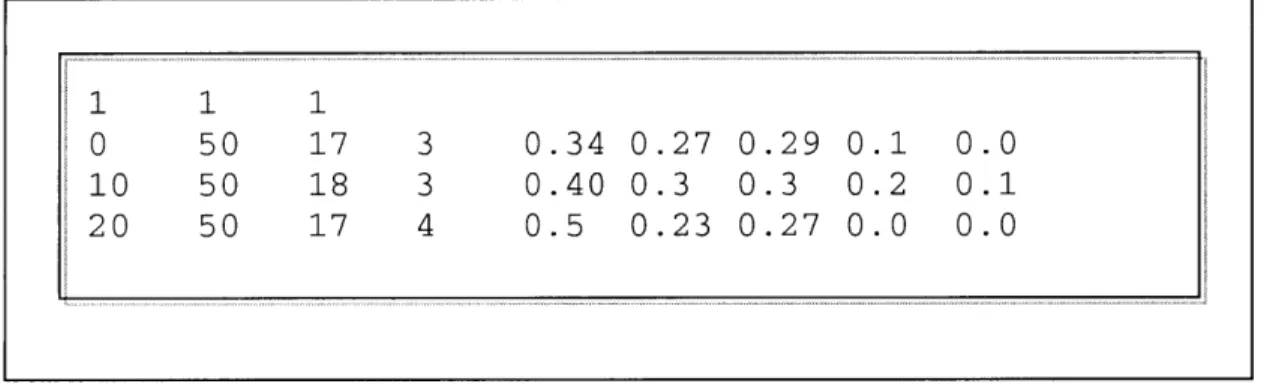
Figure 5.1 Sample of the land description file "fsurdat" for a simple

(8)

Figure 5.2 Global Distribution of 28 NCAR Land Surface Classes (NCAR CCM T42 grid). NCAR surface classes are discussed

in Section 3.2.1, and Table 3.1... 68

Figure 5.3 Global Distribution of 13 NCAR sub-grid cover types (NCAR CCM T42 grid). NCAR cover types are discussed in Section 3.2.1. Their names, which are abbreviated in the legend are given in full in Table 5.1. ... 70

Figure 5.4 Global Distribution of 13 NCAR sub-grid cover types (MIT IGSM grid). NCAR cover types are discussed in

Section 3.2.1. Their names, which are abbreviated in the legend are given in full in Table 5.1. ... 72

Figure 5.5 _{Global Distribution of 9 soil colors (NCAR CCM T42 grid,} fsurdat42). NCAR soil colors in the legend are described in

Section 3.2.3, and Table 3.3... 74

Figure 5.6 Dry and saturated soil albedo on the MIT IGSM grid,

for visible and near infrared wavelengths ... 75

Figure 5.7 Schematic of N pixels in each zonal band, for use in

precipitation factor algorithm ... 82

Figure 5.8 Precipitation Factors 86.087N -54.783N. The abbreviated cover types in the legend are named in full in Table 5.1... 84

Figure 5.9 Precipitation Factors 54.783N -23.479N. The abbreviated cover types in the legend are named in full in Table 5.1... 85

(9)

Figure 5.10 Precipitation Factors 23.479N -7.826S. The abbreviated cover

types in the legend are named in full in Table 5.1... 86

Figure 5.11 Precipitation Factors 7.826S -39.13 IS. The abbreviated cover

Figure 5.12 Precipitation Factors 39.131S -54.783S. The abbreviated cover

Figure 6.1 Annual Mean Net Longwave and Shortwave Radiation, in W m-2 as a function of latitude, derived from a 50-year simulation replacing the land component of MIT 2D-LO

with the NCAR Land Surface M odel. ... 93

Figure 6.2 Air temperature at a reference height of 2m as a function of latitude, in degrees Celsius, derived from a 50-year simulation replacing the land component of MIT 2D-LO with the NCAR Land Surface Model. The annual mean is plotted on the left, and

seasonality (July-January) on the right. Results are compared to those from the MIT-2D-LO and observations from

Leem ans and Cramer (1991). ... 96

Figure 6.3 50-year time series of annual mean air temperature in degrees Celsius, modeled using the NCAR Land Surface model over the land portion in MIT 2D-LO.Results for zonal bands centered on latitudes 82.174N to 19.566N . ... 97

Figure 6.4 50-year time series of annual mean air temperature in degrees Celsius, modeled using the NCAR Land Surface model over the land portion in MIT 2D-LO.Results for zonal bands centered on latitudes 11.740N to -50.870N ... 98

(10)

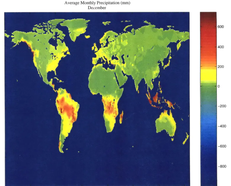
Figure 6.5 Precipitation in mm day' as a function of latitude, derived from a 50-year simulation replacing the land component of MIT 2D-LO with the NCAR Land Surface Model. The annual mean is plotted on the left, and seasonality (July-January) on the right. Results are compared to those from the MIT-2D-LO and observations from

Leem ans and Cram er (1991). ... 102

Figure 6.6 50-year time series of annual mean precipitation in degrees mm day-, modeled using the NCAR Land Surface model over the land portion in MIT 2D-LO.Results for zonal bands centered on latitudes

82.174N to 19.566N ... 103

Figure 6.7 _{50-year time series of annual mean precipitation in mm day-,} modeled using the NCAR Land Surface model over the land portion in MIT 2D-LO.Results for zonal bands centered on

latitudes 11.740N to -50.870N ... 104

Figure 6.8 _{Latent Heat Flux in W m-2 as a function of latitude, derived from a} 50-year simulation replacing the land component of MIT 2D-LO with the NCAR Land Surface Model. The annual mean is plotted on the left, and seasonality (July-January) on the right. Results are compared to those from the MIT-2D-LO and observations

from O berhuber (1988). ... 107

Figure 6.9 50-year time series of annual mean latent heat flux in W m-2 modeled using the NCAR Land Surface model over the land portion in MIT 2D-LO.Results for zonal bands centered on

latitudes 82.174N to 19.566N . ... 109

(11)

Figure 6.10 Figure 6.11 Figure 6.12 Figure 6.13 Figure 6.14 Figure 6.15 Figure 6.16

50-year time series of annual mean latent heat flux in W m-2 modeled using the NCAR Land Surface model over the land portion in MIT 2D-LO.Results for zonal bands centered on

latitudes 1 1.740N to -50.870N . ... 110

Sensible Heat Flux in W m2 as a function of latitude, derived from a 50-year simulation replacing the land component of MIT 2D-LO with the NCAR Land Surface Model. The annual mean is plotted on the left, and seasonality (July-January) on the right. Results are compared to those from the MIT-2D-LO and observations from

O berhuber (1988). ... 112

50-year time series of annual mean sensible heat flux in W m-2 modeled using the NCAR Land Surface model over the land portion in MIT 2D-LO. Results for zonal bands centered on

latitudes 82.174N to 19.566N . ... 115

50-year time series of annual mean sensible heat flux in W m-, modeled using the NCAR Land Surface model over the land portion in MIT 2D-LO. Results for zonal bands centered on

latitudes 11.740N to -50.870N . ... 116

-2

Net CO2 flux to the atmosphere in g m , as a funcion of

latitude on the y-axis and month of year on the x-axis. ... 118

Net CO2 flux in Gt CO2 as a function of latitude, derived from a

50-year simulation replacing the land component of MIT 2D-LO with the NCAR Land Surface Model. The annual mean is plotted on the left, and seasonality (July-January) on the right. ... 119

(12)

using the NCAR Land Surface model over the land portion in MIT 2D-LO. Results for zonal bands centered on latitudes

82.174N to 19.566N ... 123

Figure 6.17 _{50-year time series of annual mean CO}₂_{flux in g m-2}_,_modeled using the NCAR Land Surface model over the land portion in MIT 2D-LO.Results for zonal bands centered on latitudes

11.740N to -50.870N ... 124

Figure 7.1 Calling sequence for subroutine surphy.F... 127

(13)

List of Tables

Table 3.1 NCAR LSM Surface Classes and their constituent sub-grid cover typ e s... . . 3 8 Table 3.2 NCAR LSM Fundamental cover types and their abbreviated titles .. 40 Table 3.3 NCAR LSM Dry and Saturated Albedos as a function of

so il co lor... . . 4 1 Table 3.4 NCAR LSM Required Inputs ... 43 Table 3.5 NCAR LSM Output to Atmospheric Model ... 43 Table 4.1 Olson Ecosystem Classifications, Version 1.3... 59

Table 5.1 NCAR LSM Fundamental cover types and their abbreviated titles.. 69 Table 5.2 Required atmospheric forcing from MIT 2D-LO to NCAR LSM .... 77

(14)

Chapter 1 Introduction

The atmosphere and the terrestrial biosphere comprise a system coupled through chemical, energy and water cycles and acting on a range of temporal and spatial scales. Science questions abound in the field of climate change, and few if any can be addressed by considering one cycle without reference to the others.

In order to address the science questions about the Earth System and about future climate impacts on the global ecosystem based on models, there needs to be tighter coupling between the terrestrial ecology processes and hydrologic processes.

While climate change may be manifested in changes in surface temperature, sea level, ocean circulation patterns and occurrence of extreme climatic events, its origins rest not only in natural variability, but also in anthropogenic processes. Integrated climate models are used to simulate global environmental changes that may result from anthropogenic causes. They also allow us to study the uncertainties associated with projected changes, and the impact of proposed policies on such changes. The MIT Integrated Global System Model (IGSM) includes coupled models of atmospheric chemistry, physical climate and human activity, and it is an example of a framework within which the variability and change in climate may be quantitatively assessed. In the MIT IGSM, the combined anthropogenic and natural emissions model outputs are driving forces for the coupled atmospheric chemistry and climate model, the essential components of which are

(15)

chemistry, atmospheric chemistry, atmospheric circulation and ocean circulation. The climate outputs drive a terrestrial ecosystems model predicting land vegetation changes, land CO2 changes, and soil composition, which feed back to the coupled

chemistry/climate, and natural emissions models.

A shortcoming of the MIT IGSM is the asynchronous coupling of the land surface hydrology component and the terrestrial ecology model. At each hourly time-step the land surface hydrology component is forced with precipitation, wind, temperature, humidity and radiation input from the atmospheric component. In turn, the land surface model generates the surface moisture, energy, momentun and radiative fluxes required by the next step of the atmospheric model. On the other hand, the TEM is run on a monthly time-step, forced with monthly average precipitation, temperature and cloudiness, as well as a description of soil texture, elevation and water availability. The TEM estimates carbon and nitrogen fluxes, which are inputs to the coupled chemistry-climate model and the natural emissions model. An advantage of the NCAR LSM is that it estimates the carbon dioxide flux at each time-step, yielding a value that is consistent with the rate of evapotranspiration.

A major goal of the MIT Joint Program for Global Change Science is the evaluate

uncertainties in climate change prediction (Jacoby and Prinn, 1994). Typically, numerous versions of an atmospheric model will be used to study several scenarios for changes in greenhouse gas concentrations, resulting in a large number of 50-100 year simulations being carried out for typical studies. As Global Circulation Models (GCMs) require an

(16)

enormous amount of computer time, the current MIT Climate Model couples a two-dimensionsal (2D - zonally and vertically) land and ocean-resolving (LO) statistical-dynamical model of the atmosphere to a 3D ocean model. This simplified 2D

atmosphere/3D ocean model successfully reproduces many characteristics of the current zonally-averaged climate (Sokolov and Stone, 1995), while being twenty times faster than 3D models with similar latitudinal and vertical resolutions.

The objective of this research was to determine if the NCAR LSM could be introduced within the framework of the MIT IGSM, as a first step towards having a truly consistent coupling between the terrestrial ecosystem and the climate model. A detailed description of the relevant components of the MIT IGSM and the NCAR LSM is given in Chapters 2 and 3. Particular attention is drawn to the similarities and differences between the NCAR model and the climate and terrestrial ecology components of the MIT model.

In order to use the NCAR LSM within the framework of the MIT IGSM, it must be included as a zonally averaged model. One of the major changes in employing the NCAR LSM is the representation of the land surface. Whereas the current climate model

distinguishes between ocean, ocean ice, land and land ice, the new model will have up to fifteen land cover types within each zonal band. Model inputs that had to be adapted include geographical location, land surface parameterization, land surface type, soil color and percentage lake and wetlands. These changes are described in detail in Chapter 5, along with the changes to model architecture required to accommodate them. Factors were derived by which zonal precipitation could be adjusted to reflect the variation in

(17)

precipitation over these cover types. It is noteworthy that as the NCAR LSM is vectorized, the atmospheric forcing applied to each individual cover type could be factored without any increase in computational effort.

In order to determine the land cover distribution and the precipitation, data was

downloaded from the Global Ecosystems Database H, and used in conjunction with the data provided with NCAR LSM. These datasets are discussed in full in Chapter 4, and the resultant characterization of the global land surface and development of the precipitation scheme is described in Chapter 5.

In Chapter 6 the results from a fifty-year simulation are presented, to demonstrate that the NCAR Land Surface Model, when coupled to the GISS model produces a satisfactory climatology. The annual mean and seasonality in net radiation show that the exchange of forcing data is correct, while those of temperature and precipitation indicate that the new model yields a satisfactory meteorology while showing the same artifacts of zonal averaging as those from the old model. Some improvement is seen in the estimates of latent and sensible heat fluxes compared to those calculated by the GISS model. The estimated carbon dioxide flux from the land surface exhibits the trends associated with changing seasons and surface type distribution.

Chapter 7 contains the conclusions from this research, primarily that the NCAR LSM could be successfully coupled into the MIT IGSM. The implications of this success, in

(18)

particular the potential to expand the scope of the climate model to include estimation of biogeochemical fluxes in addition to standard climatological outputs, are also discussed. In addition, several prospective areas of future research are outlined.

(19)

Chapter 2 Coupled Climate and Ecosystem Modeling for Integrated

Assessment: The MIT IGSM

2.1 Introduction

Projected changes in future climate associated with an increase in greenhouse gases, and other chemical species such as nitrogen, phosphorous and potassium, are expected to be large enough to cause fundamental changes in ecological function and even global vegetation distribution.

Studies have also shown that changes in land cover can have a profound effect on regional climate, and possibly global climate. Therefore, the atmosphere and the

terrestrial biosphere must be considered as a system, coupled through water, energy and chemical cycles, and acting on a range of spatial and time-scales.

A typical land surface model estimates the exchange of water and energy through the turbulent sensible and latent heat fluxes and radiative transfers. A terrestrial ecology model, on the other hand is used to predict the states of plants and soils as they respond to climate change, changes in CO2 concentrations, nitrogen availability and land-use. In

particular, they simulate the carbon and nitrogen fluxes from the terrestrial biosphere when forced with climate data and a description of the land surface.

(20)

In order to investigate the evolution of climate and land-cover, in particular the interactions and feedbacks between them, the land surface parameterization and terrestrial ecology modules of any integrated global system model must be physically consistent. Typically they differ significantly in how they consider the water and energy

balances, so water and energy calculations are not always consistent.

In addition, the co-evolution of the hydroclimate and biospheric systems suggests that coupled ecological-climate models may have different equilibrium climate-vegetations regimes, and may be sensitive to ecotone initialization (Pielke, 1998).

Results from preliminary studies carried out using the existing Terrestrial Ecology Model (TEM), the MIT Joint Program on the Science and Policy of Global Change have shown that carbon storage in terrestrial ecosystems results from the superposition of a number of factors that are related to the physical climate system, biogeochemical cycles and land-use changes.

For example, when run with the land-use dataset of Ramankutty and Foley (1999), they found that historical change in land-use has led to a reduction in terrestrial carbon. During the 1980s and 1990s, terrestrial ecosystems behaved as a net carbon sink, due to the effects of CO2 fertilization. Furthermore, they have found that changes in nitrogen

dynamics and water use efficiencies caused feedbacks in the terrestrial carbon cycle, such that interactions between climate and atmospheric CO2 concentrations led to an

enhancement of this terrestrial carbon sink.

(21)

2.2 Integrated Modeling

The results discussed above prompted the need to develop the MIT IGSM to consider feedbacks between the fundamental physical and land-atmosphere processes, for example feedbacks related to carbon storage, albedo, trace gases and transpiration. Important science questions in this field include:

1) Can changes in land ecosystems caused by climate change and human activity feed back to climate and air quality through changes in albedo, terrestrial carbon storage, and trace gas exchange rates?

2) Nitrogen is a growth-limiting factor in many diverse aquatic and terrestrial ecosystems. Can coupling of the nitrogen, carbon and water cycles in land atmosphere interactions improve the ability to estimate regional evaporative fluxes in terrestrial ecosystems?

3) How do the combined effects of land-use change, atmospheric pollution, and climate change affect the productivity, carbon storage capacity and distribution of major vegetation types over the globe?

The central hypothesis of this research is that variability and change in the terrestrial component of the water cycle should be characterized in the context of the global cycles of several key macro- and micro- nutrient chemical species. The MIT Integrated Global System Model (IGSM) includes coupled models of atmospheric chemistry, physical

(22)

climate and human activity, and it is the framework within which the variability and change in the water cycle may be quantitatively assessed.

2.3 MIT Integrated Global Integrated Systems Model (IGSM)

The IGSM consists of a set of coupled sub-models of economic development and associated emissions, natural biogeochemical cycles, climate, and natural ecosystems. It attempts to include each of the major areas in the natural and social sciences that are relevant to the issue of climate change, and is designed to illuminate key issues linking science and policy.

Refer to Figure 2.1, a schematic illustrating the framework and components of the MIT Integrated Global Systems Model. Feedbacks between the submodels which are currently included are shown by solid lines, while those that are under development for future inclusion are shown by dashed lines. Output from both anthropogenic and natural emissions models drive the coupled atmospheric chemistry and climate model, which in turn drive a terrestrial ecosystems model (TEM). The TEM then predicts vegetation changes, land carbon dioxide (C02) fluxes and soil composition, which can feed back to the coupled chemistry-climate model and the natural emissions model.

(23)

Schematic Diagram of The MIT Integrated Global Systems Model (IGSM).

Source: http://web.mit.edu/globalchange/www

By carefully selecting key processes in each of the sub-models and defining the level of detail in which it must be represented, complex models for all the relevant processes can be coupled in a computationally efficient form. Such efficiency allows us to identify and understand important feedbacks between model components and to compute sensitivities of policy-relevant variables (e.g. rainfall, temperature, ecosystem state) to assumptions in

Human Activity

O

chang economlic developmrnt, p c

ows*sio , and 14nd u*V

C02 4, "+20, NOXy,

vocIS olCo. CFCs,Hf C% F fFif

Natural CHj

Emisions NjO 20 f 3 D Coupled 4

Af, AtmospherkC

*Ocean Cherltry

CO-uptake and tand

soil C Climate Processes tt

Ssoil N

rainallOceaft, atmiosphere. 6 - ,.--& land

nutrie its,

ptemperature,

r ainfall, Cloulds. COI hag

E Chsystems Processes

NPP, Veg, C, Soil N&C

(24)

Furthermore, the IGSM must be computationally feasible for use in multiple 100-year simulations, so that the future impacts on climate due to proposed policies can be examined. For simulations of this length, intra-storm variability need not be studied, so the model can be zonally averaged without any loss in accuracy.

In the following sections we will briefly introduce the components of the MIT IGSM, paying particular attention to the climate dynamics component. It is this element which we seek to improve through introduction of the NCAR Land Surface Model. Information in this chapter is largely drawn from Prinn et al. (1999), which provides descriptions of all components of the MIT IGSM.

2.4 MIT IGSM Climate dynamics (MIT 2D-LO)

The coupled climate-chemistry model is shown in Figure 2.2. The objective of the climate model is to simulate the present climate as well as reproducing the climate change patterns predicted by three-dimensional General Circulation Models (GCMs) in a more computationally efficient manner. The current MIT climate model consists of a two-dimensional (2D) land and ocean (LO) resolving statistical dynamical model of the atmosphere coupled to a three-dimensional ocean general circulation model.

(25)

Figure 2.2 Schematic Diagram of the MIT IGSM Coupled Climate-Atmospheric Chemistry Model

The 2D-LO climate model is coupled to the atmospheric chemistry model, and by running interactively and simultaneously they are capable of predicting the atmospheric concentrations of radiatively and chemically significant trace species. The coupled climate and chemistry model is 2D (latitude and altitude) with separate predictions over

land and ocean at each latitude. The grid used in the model consists of 24 points in latitude, corresponding to a resolution of 7.826 degrees. The model has nine layers in the vertical, notably two in the planetary boundary layer, five in the troposphere, and two in the stratosphere. Longitudinal variations are obtained from a combination of observed

climate data and selected transient runs of 3D climate models.

SUNLIGH

"M 'ib'MIP,

urnicit I ion "wa Ut e korl., qp e n G4S a ' 23 Of APT

(26)

Two-dimensional models certainly have some limitations when compared to 3D GCMs. For example, they are incapable of simulating features of the atmospheric circulation attributed to the temperature contrast between land and ocean. They also fail to take real topography into account. However, 2D models can be used to model climate change scenarios reasonably well if certain modifications are made.

The two-dimensional statistical dynamical model was originally developed at the NASA Goddard Institute for Space Studies (GISS). It was derived from the GISS GCM of Hansen et al. (1983). Yao and Stone (1987) provide a detailed description of the original 2D model, which they found to be 23 times faster than the GISS full GCM with similar latitudinal and vertical resolution. The most important feature of the 2D model is that it incorporates the radiation code from the GISS GCM. This code incorporates all of the significant greenhouse gases such as H20, CO2, CH4, N20, CFCs and aerosols. For use

within the MIT IGSM, several modifications were made to the GISS 2D model. These changes will be discussed below.

The name "MIT 2D-LO" derives from the first necessary change. The GISS 2D model assumed that the terrestrial boundary consisted entirely of ocean. The MIT 2D-LO, like the GISS GCM, allows up to four different kinds of surface in the same grid cell, namely ocean, ocean ice, land and land ice. The surface characteristics such as temperature and soil moisture as well as surface turbulent fluxes are calculated separately for each kind of surface while the atmosphere is assumed to be well-mixed horizontally in each grid cell.

(27)

The weighted averages of fluxes from the four surface types are used to calculate changes of temperature, humidity, and wind speed in the model's first layer due to the air-surface interaction. The same applies to the surface albedo used in radiative flux calculations.

The MIT 2D-LO model explicitly solves the primitive equations for zonal mean flow and includes parameterizations of heat, moisture, and momentum transport by large scale eddies based on baroclinic instability theory. It also includes parameterizations of all the main physical processes such as radiation, convection and cloud formation. It is thus capable of reproducing many of the nonlinear interactions taking place in GCMs.

The surface flux calculation scheme is based on Monin-Obukhov Similarity Theory, and uses the approximation for transfer coefficients derived by Deardorff (1978). Details of this scheme, and those used for ground temperature and moisture calculations are given in Hansen et al. (1983).

The main difference between the approaches of the MIT 2D-LO and that of the original GISS GSM lies in the definition of variables at the top boundary of the surface layer. In the GISS GCM, the surface layer is assumed to be in equilibrium. The numerical realization of this assumption results in a complicated algorithm including nested

iterations. This algorithm can be used in the GISS GCM and 2D-LO without land, but results in computational difficulties when land is included. Therefore in the MIT 2D-LO

the assumption of surface layer equilibrium is replaced by the assumption that the layer between the surface and the model's first layer is well-mixed.

(28)

Other differences between the MIT 2D-LO and the original GISS 2D model are a simplified wind speed calculation in the MIT model, as well as a modification to the cloud parameterization. In the original GISS 2D model, condensation occurs when humidity reaches 100%. In the MIT 2D-LO model, condensation is allowed to occur in partly saturated cells to allow for subgrid-scale variation in relative humidity. The criterion for condensation, hcon, is therefore reduced to 90%. This small changes has a

significant impact on the model's sensitivity, insofar as the model produces a negative

cloud feedback when hcon is 100%, whereas it produces a positive cloud feedback if hcon

is reduced to 90%.

Sokolov and Stone (1995) presented results of simulations with the MIT 2D-LO model, demonstrating that it could reproduce the main features of the present climate reasonably well. The objective of this project is to further improve the performance of the MIT 2D-LO by incorporating the NCAR land surface model to perform the surface flux, ground temperature and moisture calculations over the land component of each grid cell.

2.5 MIT IGSM Terrestrial Ecology Model, TEM

The carbon cycle and the nitrogen cycle play significant roles in tying changes in climate change to changes in the terrestrial biosphere. Climate change forces changes in the terrestrial biosphere, which in turn impact climate dynamics. These feedbacks are analyzed in the MIT IGSM using the Terrestrial Ecosystems Model (TEM) developed at

(29)

the Marine Biology Laboratory (MBL). A schematic diagram of TEM is given below in Figure 2.3. grmss primary productbin Figure 2.3

atmospheric carbon dioxide

respiratbn decompositbn Soil :ation and Detriftus ~prodcilcn netexdunge minerdizaidon

Nitrogen Inrani R Nitroen

Schematic Diagram of the MIT IGSM Terrestrial Ecology Model (TEM)

Source: http://web.mit.edu/globalchange /www/

The Terrestrial Ecology Model is used in the IGSM to predict the states of plants and soils as they respond to climatic variability, atmospheric CO2 concentrations, nitrogen

availability and changes in land-use. Its use within the MIT IGSM allows us to study how climate-driven changes in the terrestrial biosphere affect climate dynamics through feedbacks on both the carbon cycle and the natural emissions of trace gases.

(30)

The TEM is run on a monthly time-step, forced with monthly average precipitation, temperature and cloudiness (derived from the MIT 2D-LO model), as well as a description of soil texture, elevation and water availability. An inbuilt water balance model generates the required hydrological inputs to simulate the carbon and nitrogen fluxes over 18 terrestrial ecosystems.

The estimated carbon and nitrogen fluxes, as well as changes in vegetation cover and soil composition, are inputs to the coupled chemistry/climate model and the natural emissions model. Furthermore, this information is useful in its own right, as changes in land cover will lead to economic and ecological impacts. Climate change is reflected in changes to the carbon and nitrogen cycles, in particular carbon storage in vegetation and soils.

2.6 MIT IGSM Natural Emissions Model (NEM)

Natural terrestrial fluxes of methane (CH4) and nitrous oxide (N20) from soils and wetlands are significant contributors to the global budgets for these gases. Due to their dependence on climate, these fluxes must be modeled within the MIT IGSM. This takes place in the Natural Emissions Model.

The driving variables for the global model for N20 emissions include vegetation type, total soil organic carbon, soil texture and climate parameters. Recall from Figure 2.1 that

soil carbon and soil nitrogen were inputted to NEM from TEM, while temperature and

(31)

precipitation data was received from the climate model. In turn the CH4 and N20 fluxes

calculated in NEM are used as input to the atmospheric chemistry model.

Climatic influences, particularly temperature and precipitation, determine dynamic soil temperature and moisture profiles and shifts of aerobic-anaerobic conditions. The N20

model can predict daily emissions of N₂0, N₂, NH₃and CO2 as well as the daily soil

uptake of CH4. The N20 emissions model has a spatial resolution of 2.5 degrees.

The methane emission model was developed specifically to estimate fluxes of methane from wetlands and wet tundra. In high-latitude and tropical wetlands methane flux is modeled based on soil temperature and bog soil temperature. Methane emissions from wet tundra are calculated by assuming a constant small methane flux and an emission season based on the time period for which the surface temperature is above the freezing point.

2.7 The MIT IGSM Emissions Prediction and Policy Analysis (EPPA)

Model

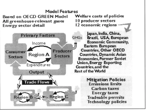
The Emissions Prediction and Policy Analysis (EPPA) Model shown in Figure 2.4 is a model of economic growth, international trade and greenhouse gas emissions. It is used to compute predictions of anthropogenic emissions of the key gases from twelve economic regions, and to provide economic analysis of proposed control measures.

(32)

Model Features

Based on OECD GREEN Model Welfare costs of policies All green h ouse-re levant gases 1 0 producer sectors Energy sector detail 12 economic regions

Japan, India, China,

GHGs Brazil, USA, European

Income Econonic Community,

Eastern European

Countries, Other OECD Region A Countries, Dynamic Asian

Economies, Former Soviet Union,Energy Exporting Countries,and the Rest of the lorld

Mitigation Policies

Emissions limits

Carbon taxes Energy taxes

inion Tradeable permits

Technology policies

Figure 2.4 Schematic Diagram of the MIT Emissions Prediction and Policy

Analysis (EPPA) Model

EPPA has been formulated to support analysis of a host of emissions control policies,

providing estimates of the magnitude and distribution among nations of the costs, and clarifying the ways that changes are mediated through international trade. Special provision is made for analysis of uncertainty in key elements, such as the growth of population and economic activity, and the pace and direction of technical change. In addition to predicting future levels of emissions of greenhouse gases and aerosols, future economical and technological change are modeled in some detail. Economic development and the consequent emissions of trace gases are predicted as functions of geographic location and time, in order to capture the impact of chemical species that exist in the atmosphere for only a short period of time.

(33)

2.8 Asynchronous coupling of hydrologic and ecological models

within the MIT IGSM

This framework has one fundamental shortcoming in that some components are linked sequentially. Therefore because the components are linked asynchronously, the output from the climate model is used to force the terrestrial ecology model. In reality, however, there are significant feedbacks between the physical climate, atmospheric chemistry and biosphere that can only be captured if these components are integrated synchronously and with coupled exchanges of mass, heat and chemical species.

(34)

Chapter 3 National Center for Atmospheric Research Land Surface

Model, Version 1.0.(NCAR LSM)

3.1 Introduction

Recall from Chapter 2 that we wish to capture the significant feedbacks between the physical climate, atmospheric chemistry and biosphere. We hope to achieve this through synchronous integration of these component models, thereby obtaining coupled

exchanges of mass, heat and chemical species.

The NCAR LSM Version 1.0 was initially developed to combine "the relevant biogeophysical, biogeochemical, hydrologic and ecosystem processes into a comprehensive model of land-atmosphere interactions that was physically and

biologically realistic and also internally self-consistent", so in principle it seems ideal for our purposes.

Furthermore, a feasibility study by deSilva (1998) using data from the FIFE experiment (Betts and Ball, 1998) demonstrated that using the same atmospheric forcing in

uncoupled mode, it provided improved estimates of surface fluxes compared to the existing climate and terrestrial ecology models. Partitioning of surface energy between

latent and sensible heat in the NCAR LSM was consistently better than the MIT 2D-LO

(35)

and the climate module of TEM at different levels of saturation. It was also found that the hydrological models in MIT 2D-LO and TEM were inconsistent; the MIT 2D-LO sub-surface was often too dry restricting evaporation, and resulting in erroneous ground temperature. The climate component of TEM, on the other hand resulted in excessive evaporation during rainy periods. DeSilva also found that as NCAR LSM calculates all fluxes and ground temperature simultaneously, its errors in ground heat flux were smaller than those of the other two models. Furthermore, the employment of a multi-layer soil column in NCAR LSM facilitated accurate ground temperature, soil moisture and surface flux calculations at both diurnal and seasonal cycles. The layered soil column was found to perform better than a merely deep soil column.

It is anticipated that the greater coupling between the climate, atmospheric chemistry and terrestrial ecology achieved by using the NCAR LSM to model the land ("L") component of the MIT 2D-LO model will allow full development of physical feedbacks, and

(36)

T, u,vq, C02, 02 H,XE

Sdown, Ldown Sup, LUP

biophysical fluxes X Y Co2 CH4, NMHC, N20 biogeochemical fluxes photosynthesis, temperature j height LAI water E, snow melt -el 0

..

I

biomass vegetation " type " height - foliage/stem/root 0 0 0. 0 soil * slow e fast

H-water - vegetation/snow/soil " wetland/lake/glacier - groundwater " river lateral outflow hydrologic transport * maintenance respiration " growth respiration - microbial respiration * net primary production

soil water veg type biomass ecosystem dynamics * phenology - growing season -monthly foliage * vegetation dynamics - growth * regeneration " mortality * soil processes * decomposition * mineralization surface/sub-surface transport river flow

lateral inflow lake/wetland/glacier dynamics ux to ocean

0 C.4 '-4 " radiative transfer - sensible/latent heat - stomatal physiology * momentum flux - soil heat/snow melt

" temperatures V column hydrology H4 Co2 fluxes NPP * interception * throughfall/stemflow - snow hydrology infiltration/surface runoff - soil water redistribution - capillary rise/drainage Sirrigation -lateral inflow - i Iveg type F

(37)

In the NCAR Land Surface Model (Version 1.0), land surface processes are described in terms of biophysical, and biogeochemical fluxes which depend on both the ecological and hydrologic state of the land. Biophysical fluxes include latent and sensible heat, momentum, reflected solar radiation and emitted longwave radiation. The flux of carbon dioxide is the main biogeochemical flux considered by the model. The processes at work in the ecological and hydrologic sub-models are shown in Figure 3.1, along with the interactions between them.

The objective of this chapter is to introduce the NCAR LSM Version 1.0.

Land Surface Characterization, typical model input and output requirements and model physics shall be discussed. For further detail the reader is referred to the Technical Description and User's Guide (Bonan, 1996).

3.2 Land Surface Characterization in NCAR LSM Version 1.0.

Each grid cell is characterized by one of twenty-eight surface classes, one of nine soil colors, soil texture information, and the fractions of the grid cell covered by lake and wetlands.

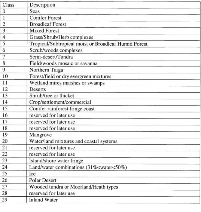
3.2.1 Land Surface Class

Each grid cell is assigned a land surface class (1-28), from those listed in Table 3.1. A surface class of zero indicates that the cell is entirely ocean, so it will not be modeled by NCAR LSM.

(38)

Table 3.1 NCAR LSM Surface Classes and their constituent sub-grid cover types

NCAR LSM Classification bare net ndt bdt tst wg ag c cg ads es ds bet

I Land ice 1 0 0 0 0 0 0 0 0 0 0 0 0

2 Desert 1 0 0 0 0 0 0 0 0 0 0 0 0

3 Cool needleleaf evergreen tree 0.25 0.75 0 0 0 0 0 0 0 0 0 0 0

4 Cool needleleaf deciduous tree 0.5 0 0.5 0 0 0 0 0 0 0 0 0 0

5 Cool broadleaf deciduous tree 0.25 0 0 0.75 0 0 0 0 0 0 0 0 0

6 Cool mixed needleleaf evergreen & 0.26 0.37 0 0.37 0 0 0 0 0 0 0 0 0

broadleaf deciduous trees

7 Warm needleleaf evergreen tree 0.25 0.75 0 0 0 0 0 0 0 0 0 0 0

8 Warm broadleaf deciduous tree 0.25 0 0 0.75 0 0 0 0 0 0 0 0 0

9 Warm mixed needleleaf evergreen & 0.26 0.37 0 0.37 0 0 0 0 0 0 0 0 0

broadleaf deciduous trees

10 Tropical broadleaf evergreen tree 0.05 0 0 0 0 0 0 0 0 0 0 0 0.95

11 Tropical seasonal deciduous tree 0.25 0 0 0 0.75 0 0 0 0 0 0 0 0

12 Savanna 0 0 0 0 0.3 0.7 0 0 0 0 0 0 0

13 Evergreen forest tundra 0.5 0.25 0 0 0 0 0.25 0 0 0 0 0 0

14 Deciduous forest tundra 0.5 0 0.25 0 0 0 0.25 0 0 0 0 0 0

15 Cool forest crop 0 0.3 0 0.3 0 0 0 0.4 0 0 0 0 0

16 Warm forest crop 0 0.3 0 0.3 0 0 0 0.4 0 0 0 0 0

17 Cool grassland 0.2 0 0 0 0 0.2 0 0 0.6 0 0 0 0 18 Warm grassland 0.2 0 0 0 0 0.6 0 0 0.2 0 0 0 0 19 Tundra 0.4 0 0 0 0 0 0.3 0 0 0.3 0 0 0 20 Evergreen shrub 0.2 0 0 0 0 0 0 0 0 0 0.8 0 0 21 Deciduous shrub 0.2 0 0 0 0 0 0 0 0 0 0 0.8 0 22 Semi-desert 0.9 0 0 0 0 0 0 0 0 0 0 0.1 0

23 Cool irrigated crop 0.15 0 0 0 0 0 0 0.85 0 0 0 0 0

24 Cool crop 0.15 0 0 0 0 0 0 0.85 0 0 0 0 0

25 Warm irrigated crop 0.15 0 0 0 0 0 0 0.85 0 0 0 0 0

26 Warm crop 0.15 0 0 0 0 0 0 0.85 0 0 0 0 0

27 Forest wetland 0.2 0 0 0 0 0 0 0 0 0 0 0 0.8

(39)

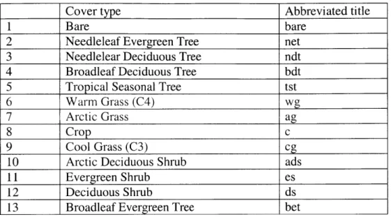
Each of the 28 surface classes consists of combination of plant types and bare soill, as shown in Table 3.1. These 13 fundamental cover types, named in full in Table 3.2, differ in important properties that influence surface fluxes, for example:

* Leaf and stem areas

" Root profile, canopy height, leaf dimension, stem and root biomass

" Physiological properties that determine stomatal resistance and CO2 fluxes " and roughness length, displacement height, and other aerodynamic properties.

The significance of this parameterization is that the model performs separate flux calculations for each fractional cover type and then averages the fluxes, instead of using bulk parameters to characterize the whole cell. Surface types were derived from the 0.50 x 0.50 dataset of Olson et al. (1983). Vegetation composition and fractional areas are

currently time-invariant.

It is apparent from Table 3.1 that several surface classes are comprised of the same fractions of sub-grid cover. For example cool broadleaf deciduous forest is identical to warm broadleaf deciduous forest. This is because in the current version of the model there is no physiological differences between cool and warm plant types, except cool C₃ and warm C4grasses.

(40)

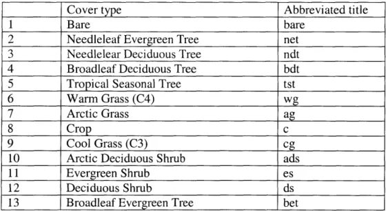
Cover type Abbreviated title

1 Bare bare

2 Needleleaf Evergreen Tree net

3 Needlelear Deciduous Tree ndt

4 Broadleaf Deciduous Tree bdt

5 Tropical Seasonal Tree tst

6 Warm Grass (C4) wg

7 Arctic Grass ag

8 Crop c

9 Cool Grass (C3) cg

10 Arctic Deciduous Shrub ads

11 Evergreen Shrub es

12 Deciduous Shrub ds

13 Broadleaf Evergreen Tree bet

Table 3.2 NCAR LSM Fundamental cover types and their abbreviated titles

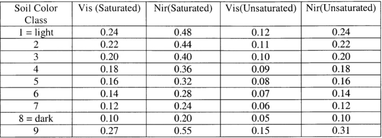
3.2.2 Soil Color

The soil in each grid cell must be assigned a color, 1 to 9. The color of the soil

determines its albedo in a dry or saturated state, at visible and near-infrared wavelengths as shown in Table 3.3. The first eight color classes are as in BATS (Dickenson et al., 1993). The ninth class is particular to desert and semi-desert surface types in North Africa and the Arabian Peninsula. In order to match ERBE clear-sky albedos, albedo was increased by 0.1.

(41)

Soil Color Vis (Saturated) Nir(Saturated) Vis(Unsaturated) Nir(Unsaturated) Class 1 = light 0.24 0.48 0.12 0.24 2 0.22 0.44 0.11 0.22 3 0.20 0.40 0.10 0.20 4 0.18 0.36 0.09 0.18 5 0.16 0.32 0.08 0.16 6 0.14 0.28 0.07 0.14 7 0.12 0.24 0.06 0.12 8 = dark 0.10 0.20 0.05 0.10 9 0.27 0.55 0.15 0.31

Table 3.3 NCAR LSM Dry and Saturated Albedos as a function of soil color

3.2.3 Soil Texture

The soil texture within each grid cell is inputted to the model by prescribing the percentages of sand, silt and clay in the grid cell. Describing soil texture in this form enables the model to account for the effect of different soil types. Thermal properties such as heat capacity and thermal conductivity, and hydraulic properties such as porosity, saturated hydraulic conductivity, saturated matric potential and the slope of the retention curve, are functions of soil texture.

3.2.4 Percentage Lakes and Wetlands

The fraction the grid cell covered in lake or wetlands must also be prescribed to fully characterize the cell. If present, lake and/or wetlands form additional sub-grid patches.

Lakes may be either deep (50m) or shallow (10m). In Version 1.0, all lakes are modeled as deep lakes.

(42)

3.3 Required Atmospheric Forcing, and Typical Output of NCAR

LSM

The NCAR LSM Version 1.0 was designed to be coupled with the NCAR CCM3. Full coupling between the atmospheric model and the land surface model is achieved through a fully explicit time-stepping procedure.

The current state of the atmosphere is used to force the land model. The required inputs are listed in Table 3.4. The Land Surface Model uses these to calculate the surface energy, constituent (water vapor and carbon dioxide), momentum and radiative fluxes required by the next step of the atmospheric model. When coupled to CCM3, the outputs from NCAR LSM listed in Table 3.5 are used to force the next step of the CCM3.

(43)

Quantity Symbol Units

Reference height Zatm m

Temperature at Zatm Tatm K

Zonal wind at Zatm Uatm M S1

Meridional wind at Zatm Vatm M s-1

Specific Humidity at Zatm qatm kg

kg-Pressure at Zatm Patm Pa

Partial pressure CO2 at zatm 355 x 10-6 mol

mol-Partial pressure 02 at Zatm 0.209 mol

mop-Surface pressure Psrf Pa

Convective precipitation qprcc mm H20 s-Large-scale precipitation qprci mm H20 s-1 Incident direct bean solar Satmt

vis" W m2 radiation < 0.7gm

Incident direct beam solar Satmlni W m2 radiation 0.7 gm

Incident diffuse solar Satmbvis W m2

radiation < 0.7gm

Incident diffuse solar Satmdnir W m-2

radiation 0.7 gm

Incident longwave radiation Latml W m-2

Table 3.4 NCAR LSM Required Inputs

Quantity Symbol Units

Latent heat flux XE W m-2

Sensible heat flux H W m2

Constituent flux H20, CO2 kg m-2 s-'

Zonal momentum flux X kg m 2 s-1

Meridional momentum flux TY kg m-2 s'

Emitted longwave radiation LT W m2

Direct beam albedo <0.7pm ITvis

Direct beam albedo IThnir

0.7pm

Diffuse albedo <0.7pm _ITis Diffuse albedo 0.7pm ITInir

Table 3.5 NCAR LSM Output to Atmospheric Model, when coupled to NCAR Community Climate Model

(44)

3.4 NCAR LSM Model Physics

3.4.1 Radiative fluxes

The net radiation at the surface R,, is given by

R S + (3.1)

where S and L are the net solar and net longwave fluxes absorbed by vegetation (subscript v) and (subscript g).

Photosynthesis and transpiration depend non-linearly on solar radiation, via the light response of stomata. A common way of approaching the closely related CO2 and H20 fluxes within the canopy is to divide the canopy into a sunlit fraction fsu and a shaded fraction, fsha, defined in

1- e-K(L+S) K(L + S)

fha 1- f", (3.3)

The leaf and stem index is denoted (L+S), K is a function of the amount of scattering within the canopy (Sellers, 1985), and the term e-K(L+S) is the fractional area of "sunflecks" on a horizontal plane below the leaf and stem index.

The solar radiation absorbed by the vegetation in the visible waveband is partitioned between the sunlit and shaded leaves to calculate the average absorbed photosynthetically

(45)

active radiation for sunlit (4""' ) and shaded (0"") leaves. It is assumed that the sunlit

leaves absorb the direct beam radiation, that all leaves absorb diffuse radiation, and that

leaves absorb L of the radiation absorbed by the vegetation.

L+S

The net longwave radiation (L) at the surface is calculated differently for vegetated and non-vegetated surfaces. For non-vegetated surfaces it is given by Equation 3.4:

L=-a , ,r+Ego 4 (3.4)

where a. is the ground absorptivity, E, is the ground emissivity, Ti is the ground temperature in Kelvin, and a is the Stefan-Boltzmann constant (Wm-2_K-4).

For vegetated surfaces, the net longwave radiation flux has components from the vegetation and the ground:

L = L,+ L9 (3.5)

where

L = -a (Lat,, +L, )+ 2E,, ,T,4 (3.6)

L, =-a, (L,, b)+ E, 4 (3.7)

The subscrips v denote from the canopy, and g denotes from the ground. The downward flux from the canopy is given by

LT, = ( - at)Li,, I +E 4 gT u (3.8)

(46)

L, T=(1--ag,)Lv I +EgCFT,4 g g (3.9)

3.4.2 Turbulent fluxes

The expressions used to estimate the surface fluxes are derived by applying Monin-Obukhov similarity theory separately to the vegetated and non-vegetated surfaces and

combining the results.

The zonal and meridional momentum fluxes, rX and rY are given by

Pt = -pam (uatm -u ) (3.10) ram Pr = -Ptm (Va,, - V, ) (3.11) ram

where u am _{and vatm are the zonal and meridional winds (ms-1) at a reference height zatm} us and vs are the zonal and meridional winds (m s-1) at the surface, and ra.n is the

aerodynamic resistance (s m-1) for momentum between the surface and the reference height zo,,,+d (the apparent sink for momentum).

For non-vegetation surfaces (where L+S=0), the sensible and latent heat fluxes are given

by

H =-Patm,, CP """ (3.12)

rah

AE Patm Cp Leat, e(g (3.13)

Y raw + rjr

where in Equation (3.12) Tg is the ground temperature(K) and is equivalent to the surface temperature T, here, attn is the potential temperature (K) at the reference height _Zatrn,_Parn

(47)

is the density of moist air (kg m-3), C, is the heat capacity of air (J kg' K1), ral, is the aerodynamic resistance to sensible heat transfer between the atmosphere at height Zatn

and the surface at height zol,+d (the apparent sink for heat). In Equation (3.13), y is the psychrometric constant (Pa K-), eat,ni is the vapor pressure (Pa) at height Zatm,, e,(Tg) is the

saturation vapor pressure (Pa) at the ground temperature, raw is the aerodynamic

resistance to water vapor transfer between the atmosphere at a height Zatn and the surface at a height zo,,+d (the apparent sink for water vapor), rsf is a surface resistance (s m1) that accounts for water vapor transfer between the soil with water vapor pressure e,(Tg) and the apparent sink for water vapor with a vapor pressure e.

For vegetated surfaces, H and AE are partitioned into vegetation and ground fluxes that depend on vegetation T, and ground T, temperatures in addition to surface temperature T, and vapor pressure e. Sensible heat flux is given by

H = Hv +Hg (3.14) where 2(L + S ) H -patmC(T -Tv ) ( - (3.15) rb Hg = -pa,,CP (3.16) rah