Image reconstruction from limited range projections using orthogonal moments

HAL Id: hal-00135856

https://hal.archives-ouvertes.fr/hal-00135856

Submitted on 12 Mar 2014

HAL is a multi-disciplinary open access archive for the deposit and dissemination of sci-entific research documents, whether they are pub-lished or not. The documents may come from teaching and research institutions in France or abroad, or from public or private research centers.

L’archive ouverte pluridisciplinaire HAL, est destinée au dépôt et à la diffusion de documents scientifiques de niveau recherche, publiés ou non, émanant des établissements d’enseignement et de recherche français ou étrangers, des laboratoires publics ou privés.

Image reconstruction from limited range projections

using orthogonal moments

Huazhong Shu, Jian Zhou, Guo-Niu Han, Limin Luo, Jean-Louis Coatrieux

To cite this version:

Huazhong Shu, Jian Zhou, Guo-Niu Han, Limin Luo, Jean-Louis Coatrieux. Image reconstruction from limited range projections using orthogonal moments. Pattern Recognition, Elsevier, 2007, 40 (2), pp.670-680. �10.1016/j.patcog.2006.05.035�. �hal-00135856�

Image reconstruction from limited range projections

using orthogonal moments

H.Z. Shua, J. Zhoua, G.N. Hanb, L.M. Luoa, J.L. Coatrieuxc

a

Laboratory of Image Science and Technology, Department of Computer Science and

Engineering, Southeast University, 210096, Nanjing, China

b

IRMA, Université Louis Pasteur et C.N.R.S., 7, rue René-Descartes F, 67084 Strasbourg,

France

c

Laboratoire Traitement du Signal et de l’Image, Université de Rennes I – INSERM U642,

35042 Rennes, France

Information about the corresponding author:

Huazhong Shu, Ph.D

Laboratory of Image Science and Technology

Department of Computer Science and Engineering

Southeast University, 210096, Nanjing, China

Tel: 00-86-25-83 79 42 49

Fax: 00-86-25-83 79 26 98

Abstract: A set of orthonormal polynomials is proposed for image reconstruction from

projection data. The relationship between the projection moments and image moments is

discussed in detail, and some interesting properties are demonstrated. Simulation results

are provided to validate the method and to compare its performance with previous works.

Keywords: Image reconstruction, Radon transform, projection moments, image moments,

orthonormal polynomials

1. Introduction

In its classical formulation, computerized tomography (CT) deals with the

reconstruction of an object from measurements which are line integrals of that object at

some known orientations. This formulation has found many applications in the fields of

medical imaging, synthetic aperture radar, electron-microscopy based tomography, etc

[1]. The Radon transformation, due to its explicit geometric meaning, has played an

important role.

In the past decades, a number of studies have been carried out on this subject. Lewitt

has summarized a series of projection theorems [2], a detailed description about the

properties of Radon transform and its relationship to other transforms have been given by

Deans [1]. Major contributions have been reported in the biomedical engineering

new X-ray source-detector trajectories (typically a spiral for CT) and to deal with

truncated [3] and cone-beam projections [4].

Recently, the moment-based approaches to tomographic reconstruction have attracted

considerable attention of several research groups. Salzman [5] and Goncharev [6]

respectively proposed the methods based on the moments to find the view angle from the

projection data. Milanfar et al. [7] described a variational framework for the tomographic

reconstruction of an image from the maximum likelihood estimates of its orthogonal

moments. Basu and Bresler [8, 9] discussed the problem of recovering the view angles

using moments of the projections. Wang and Sze [10] proposed an approach based on the

relationship between the projection moments and the image moments to reconstruct the

CT images from limited range projections. In the Wang’s algorithm, the geometric

moments were used and interesting results have been obtained. However, the use of the

geometric moments has the following disadvantages: (1) the geometric moments of an

image are integrals of the field shape over space, and the image can be uniquely

determined by the geometric moments of all orders. They are sensitive to digitization

error and minor shape deformations [11]; (2) the geometric moments are basically

projections of the image function onto the monomials xnym. Unfortunately, the basis set

{xnym} is not orthogonal. These moments are therefore not optimal with regard to the

information redundancy and other useful properties that may result from using orthogonal

algorithm, a new moment-based approach using the orthogonal basis set to reconstruct

the image from limited range projection.

The paper is organized as follows. A brief review of Radon transform and the

definition of projection moments and image moments are given in Section 2. In Section 2,

we also establish the relationship between projection moments and image moments and

discuss how to estimate the projection moments at any specific view from image

moments. Simulation results are provided in Section 3. Section 4 concludes the paper and

provides some additional perspectives.

2. Method

We first sketch the basics of Radon transform. The orthogonal projection moments,

defined in terms of normalized polynomials, are then introduced in subsection 2.2. Some

theorems relating projection and image moments are reported and demonstrated in

subsection 2.3. In the last subsection, we show how to estimate the unknown projections

from the calculated image moments.

2.1 Radon transform

Let f(x, y) ! L2(D) be a square-integrable function with support inside the unit circle

""

+ ! =

D f x y x y s dxdy

s

g( ,#) ( , )$( cos# sin# ) (1)

where "(") denotes the Dirac delta function, s is the distance from the origin to the ray, and ! is the angle between the x-axis and the ray.

For a given view !, the two-dimensional (2D) function g(s, !) becomes a one-variable of s, denoted by g_!(s). Since g_!(s) represents a collection of integrals along a set of

parallel rays, it is also called parallel projection of g(s, !) at view ! [10]. The Radon transform given by Eq. (1) can be rewritten as

₌

""

₊ !

D f x y x y s dxdy

s

g_#( ) ( , )$( cos# sin# ) (2)

2.2 Orthogonal projection moments and image moments

The moments of g_!(s) are called projection moments in the Radon domain [2]. In this

paper, we use a set of orthonormal polynomials instead of the set of monomials {sp} to

define the projection moments. Let {Pp(s)}, p = 0, 1, 2, … #, be a set of orthonormal

polynomials defined on the interval [–1, 1], the pth order orthonormal projection moment

of g_!(s) is defined as Lp( ) Pp(s)g (s)ds 1 1 ! !

_"

# = (3)

Let #nm be the (n + m)th order orthogonal moment of f(x, y) defined as [12]

P x P y f x y dxdy

D n m

nm =

!!

( ) ( ) ( , )

" (4)

dsdxdy s P s y x y x f dxdyds s P s y x y x f L p D D p p ) ( ) sin cos ( ) , ( ) ( ) sin cos ( ) , ( ) ( 1 1 1 1 ! + = ! + =

"" "

" ""

! ! # # $ # # $ # (5)

Using the property of delta function, we have

₌

!!

₊

D p

p P x y f x y dxdy

L (") ( cos" sin") ( , ) (6) This last equation will allow us to establish a relationship between the orthogonal

projection moments defined by Eq. (3) and the orthogonal moments of f(x, y) defined by

Eq. (4). This is the objective of the next subsection.

2.3 Relationship between projection moments and image moments

Let us first introduce some basic definitions. Let the pth order normalized

polynomials Pp(t) be

!

= = p r r pr p t c t P 0 ) ( (7) and let T p p t P t P t P t P t V ( )₌( ₀( ), ₁( ), ₂( ),..., ( )) and p T p t t t t M ( )₌(1, , 2,..., ) where the subscript T indicates the transposition, then we have

Vp( )= pMp( ) (8)

where Cp = (ckr), with 0 $ r $ k $ p, is a (p + 1) % (p + 1) lower triangular matrix.

Since all the diagonal elements of Cp, ckk, are not zero, the matrix Cp is non-singular,

thus

Mp(t)=Cp1Vp( )=DpVp( )

where Dp = (dkr), with 0 $ r $ k $ p, is the inverse matrix of Cp.

Eq. (9) can be rewritten as

!

= = k r r kr k t P d t 0 ) ( , for 0 $ k $ p (10)

We then have the following theorem about the projection moments and image

moments:

Theorem 1. The orthogonal projection moment of order p at given view !, Lp(!), can be

expressed as a linear combination of image moments of same order and lower, i.e.,

!!

= " = = p n n p m nm nm p p L 0 0 ) , ( ) ($ µ $ # (11) where

(

) (

n r

)

m q r m n p q q r m r q m n r n m n q p nm r n q m n d d c p + + " + " = = " + + + +

" "

_&&'( + ₊+ _##$% = ) ) ) µ ( , ) cos sin ) ( 0 0 , , , (12)

The proof of Theorem 1 is deferred to Appendix A.

Theorem 1 can also be expressed in matrix form. To do this, let us introduce the

notations: "_M(!)=

[

_L0(!),_L1(!),...,_LM(!)

]

T ,

[

k k k k

]

T k 0 1 , 1 1 , 1 0 ) ( , ,..., ,! ! ! ! ! = " " , and

[

]

T M M ) ( ) 1 ( ) 0 ( ,..., ,! ! ! =

" where M denotes the maximum order of moments we want

to utilize. Then, we have

"_M(

#

)₌!_M(

#

)!_M (13) where TM(!) is a matrix of size (M+1) % (M+1)(M+2)/2 whose definition is given by

! ! ! ! ! ! " # $ $ $ $ $ $ % & = ! ! ! ) , ( ) , ( ) , ( ) , ( ) , ( ) , ( ) , 2 ( ) , 2 ( ) , 2 ( ) , 2 ( ) , 2 ( ) , 2 ( ) , 1 ( ) , 1 ( ) , 1 ( ) , 0 ( ) ( 02 11 20 01 10 00 02 11 20 01 10 00 01 10 00 00 ' µ ' µ ' µ ' µ ' µ ' µ ' µ ' µ ' µ ' µ ' µ ' µ ' µ ' µ ' µ ' µ ' M M M M M M T_M (14)

Here µnm(p, !), with 0 $ n, m, p $ M, are defined by Eq. (12).

Theorem 1 not only provides the solution for finding the projection moments from

image moments, but also the solution for finding image moments from projection

moments. Concerning this latter point, we have the following proposition:

Proposition 1. Given line integral projections of f(x, y) at m different angles !i in [0, $), 1

$ i $ m, one can uniquely determine the first m moment vectors #(k) _{of f(x, y), 0 $ k < m.}

This can be done using only the first m orthogonal moments Lp(!i), 0 $ p < m of the

projections.

For the proof of Proposition 1, we refer to Milanfar et al. [7].

Note that Theorem 1 is valid for any type of polynomials and therefore the

reconstruction based on geometric moments is a particular case of the problem

considered here. In fact, for the geometric moments, the coefficients ckr and dkr in Eqs. (7)

and (10) are given by

ckr =dkr =!kr (15)

where "kr is the Kronecker symbol.

In this case, Eq. (12) becomes

(

) (

n

)

m

(

) (

n

)

p n m n p nm n p c n m n p ₊ ! ""# $ %%& ' = ""# $ %%& ' + = ( ( ( ( (

In the remaining part of the paper, we focus on the use of orthogonal polynomials. In

particular, we are interested in the normalized Legendre polynomials. The pth order

normalized Legendre polynomial Pp(x) over [–1, 1] is defined by

"

= = ! + = p r r pr p p p p p x c x dx d p p x P 0 2 ) 1 ( ! 2 1 2 1 2 ) ( (17) with

_[

_{] [}

_]

! " ! # $ % % + % + + % = % odd for 0, even for , ! ! 2 / ) ( ! 2 / ) ( )! ( 2 1 2 1 2 ) 1 ( ( )/2 r p r p r r p r p r p p c p r p pr (18)

An essential step when applying a special polynomial to the reconstruction problem is to

find the inverse matrix Dp in Eq. (9). For the normalized Legendre polynomials, we have

Proposition 2. For the lower triangular matrix Cp whose elements ckr are defined by Eq.

(18), the elements of the inverse matrix Dp are given as follows

[

]

! ! " ! ! # $ % % + + % + =

&

% = % odd for 0, even for , )! 2 ( ! ! ) 1 2 2 ( ! 2 / ) ( 2 1 2 2 2 / ) ( 1 2 1 2 3 r k r k r r k j r r k r d k r j k r kr , 0 $ r $ k $ p (19)

The proof of Proposition 2 is deferred to Appendix A.

Based on the above proposition, we are now ready to give an explicit expression of

µnm(p, !) in Eq. (12) for orthonormal Legendre polynomials. Let

!!" # $$% & + + + = + + + + ' r n q m n d d c m n p _{pq n m n rn m q rm} qr( , , ) , , , ( (20)

!_qr(p,n,m)=0 for q or r being odd number (21) Eq. (12) can thus be rewritten as

!

" +

!

(

) (

)

= = " + + = ( ) 0 0 ( , , )cos sin ) , ( p n m q q r r q m r n qr nm p # $ p n m # # µ (22)

where the notation

"

! +

= ) ( 0 m n p

q stands for the summation with respect to the even value of

q varying from 0 to p – (n+m).

Substitution of Eqs. (18) and (19) into (20) yields

[ ]

[

( )/2

] [

!( )/2

] [

!( )/2

]

! )! 2 / ( )! ( )! 2 ( )! 2 ( ! ! ) 1 2 2 ( ) 1 2 2 ( 1 2 ) 1 ( ) 1 2 )( 1 2 ( ) 1 2 ( 2 ) , , ( 2 / 1 ) ( 1 2 / 2 / ) ( q m n p q m n p r q r q m n p m n m n j m i n m n p m n p r i r q j q m n p q m n p qr + + + ! ! ! ! + + + " + + + + ! + + + =

#

#

= ! = + ! ! + + ! " (23)

The apparent complexity of Eq. (23) can be omitted by the following recurrence relations

( , , ) ) 3 2 )( 2 ( ) )( 1 ( ) , , ( , 2 p n m r q m r q q m n p q m n p m n p qr r q " " + ! + + ! ! ! ! + + + + ! = + (24) ( , , ) ) 3 2 )( 2 ( ) 1 2 )( ( ) , , ( 2 , p n m r n r r q m r q m n p qr r q " " + + + + ! + ! ! = + (25) ( , , ) 3 2 ) 1 )( ( ) 5 2 )( 1 2 ( 1 ) , 2 , ( ₀₀ 00 p n m n m n p m n p n n m n p " " + + + + ! ! + + ! = + (26) ( , , ) ) 3 2 )( 1 2 ( ) 1 2 )( 1 2 ( ) 1 , 1 , ( ₀₀ 00 p n m n n m m m n p " " + + + ! = ! + (27)

[

( )/2

] [

!( )/2

]

! )! ( )! 2 ( )! 2 ( ! ! 2 ) 1 ( ) 1 2 )( 1 2 ( ) 1 2 ( 2 ) , , ( 2 / ) ( 00 m n p m n p m n p m n m n m n p m n p m n p m n p + + ! ! + + ! + + + = _{! !} ! ! " (28)

In real situations, projections from certain views are known while projections from

other views are unknown. To distinguish them, we adopt here the same terminology used

in [10]. The projections are called given projections if the views are given views; the

unknown projections correspond to the projections whose views are unknown. In the

previous subsection, we have discussed the relationship between the given projection

moments and the image moments. The following shows how to compute the unknown

projections from the image moments.

When the orthonormal polynomials Pp(s) are used in Eq. (3), the orthogonality

property leads to the following inverse transform

!

" = = 0 ) ( ) ( ) ( p p p P s L s g_# # (29)

Eq. (29) calculates g_!(s), or g(s, !), from its projection moments. If only the projection moments of order up to M are used, Eq. (29) is approximated by

!

= = M p p p P s L s g 0 ) ( ) ( ) ( ~ _" " (30)

Substituting Eq. (11) into (30), we have

!

!!

= " = = = p n n p m nm nm M p p s p P s g 0 0 0 ) , ( ) ( ) ( ~ _{µ $ #} $ (31)

where µnm(p, !) are defined by Eq. (12). Note that when the orthonormal Legendre

polynomials are used, Eqs. (22) and (23) allow to compute µnm(p, !).

view and image moments. To summarize, the projections of unknown views can be

estimated from given projections as follows

1) Compute the image moments of order up to M from given M+1 views;

2) Calculate the unknown projections from the image moments of order up to M by using Eq. (31).

3. Results 3.1 Simulations

We first apply the proposed solution to a simulated phantom f(x, y), shown in Fig. 1,

in order to compare the two methods for computing the image moments. The first method

is directly based on Eq. (4) since the image is known, the orthonormal Legendre moments,

#nm, of order up to 15 are calculated using Eq. (4). The other one is achieved through the

computation of projection moments. A projection simulation program is used to generate

all the projections from 15 given views and the image moments can then be computed

using Proposition 1. The moment values using these two methods are shown in Table 1,

where the values without parentheses are computed from the image itself, and the values

with parentheses are obtained from projection moments. It can be seen from this table

that the errors between the real image moments and calculated image moments are small.

When the image moments of order up to M are calculated, Eq. (31) is used to estimate

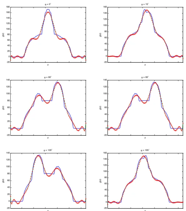
the projection moments, g~_!(s), at any specified view !. In order to test the robustness of the proposed method, we first consider the case where all the projections are known in

the interval [0, $). The estimation of g~_!(s) from the image moments with maximum order M = 15 at views of 00, 150, 600, 900, 1200 and 1650 is shown in Fig. 2. For comparison, the real projections (computed by a projection simulation program) and the

estimation results from these views using the geometric moment-based method proposed

by Wang and Sze [10] are also shown in this figure. Fig. 2 shows that the results obtained

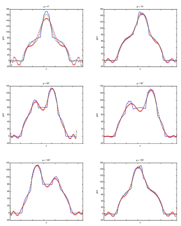
by the proposed method and Wang’s algorithm are almost the same. We then assume that

projections are available in the range of 200 $ ! $ 1600, but unknown in the ranges 00 $ ! < 200 and 1600 < ! $ 1790. The results using both the proposed method and Wang’s method are illustrated in Fig. 3. It can be observed that our method performs better than

Wang’s method, especially at views 00, 150 and 1650.

In the second example, we consider the image reconstruction problem from limited

range projections. The filtered backprojection (FBP) algorithm is used in the

reconstruction process. Since this algorithm requires the projection, g_!(s) or g(s, !), for all

s and all ! in the whole interval [0, $), we use the image moment method to estimate the

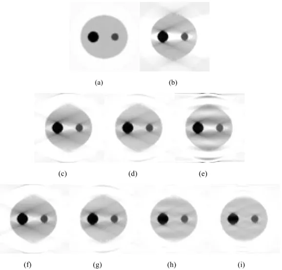
unknown projections. The original grey level image of size 128 % 128 is depicted in Fig. 4(a) (it is the same as that used in the previous example), the projections being assumed

known from 250 to 1550. A projection simulation program is applied to compute the given projection in which the following configuration is used: (a) the total view varies from 00 to 1790; (b) the angularsampling rate is 10 per view; (c) the ray sampling rate is 128 rays per view. Fig. 4(b) shows the reconstructed image from incomplete projections (250-1550)

We then use the method proposed in the previous section as well as the Wang’s

method for calculating the image moments with maximum order M equaling to 5, 10, 15,

and 20, respectively. These moments are then used to estimate the unknown projections.

Based on the given projections and the estimated projections (00-250 and 1550-1790 for this example), the FBP method is applied to reconstruct the image. The reconstructed

images based on both the proposed method and Wang’s method are illustrated in Fig.

4(c)-(i). It can be visually seen that our method leads to better results for the same value

of M. Note that the quality of the reconstructed image for Wang’s method with M = 20 is

poor due to the numerical instability, so that we have not shown this result in Fig. 4. We

also use the mean square error (MSE) to qualitatively measure the difference between the

original image and the reconstructed image. The MSE is defined as follows

(%) ₂ 100% 2 * ! " = f f f MSE (32)

where f is the original image, and f* is the reconstructed image.

Table 2 shows the MSEs for the proposed method and Wang’s method with different

values of M. The values of MSE again demonstrate the better performance of the

proposed method compared to Wang’s method.

3.2 Evaluation on “pseudo-real” data

experimentation has been conducted using a reconstructed Computed Tomography image

depicted Fig 5(a). The image intensity values (e.g. density levels) have been inverted in

order to enhance the internal details of the brain slice and the tumor features. We have

applied a two steps procedure: (i) the projection set has been computed by using a parallel

geometry (thus the so-called “pseudo-real” data) over the limited angular range; (ii) the

above reconstruction algorithms have then been used.

In this example, the projections are assumed to be known on the interval [%, 1800 – %]

where % is an adjustable parameter. We apply the proposed method to compute the image moments of order up to M = 25 for % equaling to 50, 100, 150, 200, 250 and 300, respectively. These moments are then used to estimate the unknown projections

according to (31). The reconstructed images based on both the proposed method and FBP

method are depicted in Fig. 5(b)-(m). Table 3 shows the corresponding MSEs for both

methods. Note that in the images reconstructed using FBP method (Fig. 5(b)-(g)), the

image intensity value of the unknown projections is assigned to 0. It can be observed

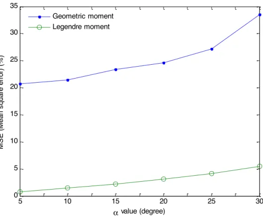
from Fig. 5(h)-(m) that the proposed method leads to good results even for large % . In order to compare the performance of the proposed method with Wang’s method,

we calculate the image moments of order up to M = 15 for different values of % (% = 50

,

100, 150, 200, 250 and 300); these moments are then used to estimate the unknown projections. The MSEs of the reconstructed imaged using FBP method for both methods

capability from limited range projections.

4. Discussion and Conclusion

In this paper, by extending Wang’s method, we have proposed a new approach based

on the orthogonal moments to solve the tomographic reconstruction problem from limited

range projections. By demonstrating some properties of Legendre polynomials, we have

established the relationship between the orthogonal projection moments and orthogonal

image moments. This relationship permits us to estimate the unknown projections from

the computed image moments so that the reconstruction problem from limited range

projections can be well solved.

It has been shown that orthogonal moments have some merits in comparison with the

geometric moments. First, the geometric moments, especially at high order, are sensitive

to noise and digitization error. Second, the orthogonal moments have simple inverse

transform, thus, the image can be more easily reconstructed from the orthogonal moments.

This new approach was evaluated through a fully known phantom and a sample of

“pseudo-real” data set. Experimental results have shown that our method is efficient, and

provides better reconstruction results compared to Wang’s method.

Reconstruction from limited range projections is of relevance for a number of medical

imaging modalities, in particular for X-ray devices. Systems such as Electron Beam

projections and allow decreasing the radiation dose for the patient, an important health

care constraint. However, the use of sparse data leads to more visible reconstruction

artifacts. A compromise is then required in order to preserve the relevant information. We

have not addressed in this paper the issue regarding the minimal number of range

projections from which a reasonable reconstruction could be obtained using the above

methods. This is a difficult problem because it can not be addressed by MSE computation

alone; subjective analysis by physicians in order to evaluate the medical consequence of a

loss of informational contents is also of major importance. It also depends on the targeted

use: when diagnosis requires high reconstruction performance, interventions may accept

lower precision in reconstruction as far as faster algorithms are available. The works in

progress are therefore devoted to such issues and also the comparison with other

reconstruction algorithms (in complexity for instance) and the performance that can be

expected for vascular reconstruction when dealing with a modality like Rot X. They also

focus on the extension of the method to other projection modes such as cone-beam

projections.

Acknowledgements: This work was supported by National Basic Research Program of

China under grant, No. 2003CB716102, the National Natural Science Foundation of

China under grant No. 60272045 and Program for New Century Excellent Talents in

Appendix A

Proof of Theorem 1. Using Eq. (7), Eq. (6) can be rewritten as

(

) (

)

x y dxdy r q c y x f dxdy y x c y x f L D p q q r r q r r q r pq D p q q pq p

!!

""

!!

"

= = # # = $$% & ''( ) = + = 0 0 0 sin cos ) , ( ) sin cos ( ) , ( ) ( * * * * * (A1) where )! ( ! ! r q r q r q ! = ""# $ %%& '

is the combination number.

Using Eq. (10), we have

(

) (

)

(

) (

)

(

) (

)

!!

"" " "

!!

""

""

""

""

!!

= # = = + # = # # = = = # = # # = # = # # = = $$% & ''( ) = $$% & ''( ) = $$% & ''( ) = D n m p n n p m p m n q m q n r m r q rn r q r pq D n m p q q r r n r q m m r q rn r q r pq r n r q m m n m r q rn r q r p q q r pq D p dxdy y x f y P x P d d r q c dxdy y x f y P x P d d r q c dxdy y P x P d d r q c y x f L ) , ( ) ( ) ( sin cos ) , ( ) ( ) ( sin cos ) ( ) ( sin cos ) , ( ) ( 0 0 , 0 0 0 0 , 0 0 , 0 0 * * * * * * * (A2)

By using Eq. (4) and by changing the variables q₌q!₊n₊m and r ₌r!₊n in the last equation of the above expression, we obtain

(

) (

)

_nm p n n p m m n p q q r m r q n r m m r q n n r m n q p p n r m n q d d c L "

## # #

" " ! = $ = + $ = = + $ + + $ + + + %%& ' (() * + + + = 0 0 ) ( 0 0 , , , cos sin ) ( (A3)

The proof is now achieved. ฀

Proof of Proposition 2. To prove the proposition, we need to demonstrate the following

kl k l r rl krd c ₌!

"

= for 0 $ k, l $ p (A4) From Eqs. (18) and (19), it is obvious that Eq. (A4) is true when the two integers k and l

have different parity. Thus, we need only to demonstrate it for the following two cases: (1)

k, r and l are all even numbers; (2) k, r and l are all odd numbers. We consider the first

case. Let k = 2u, r = 2v and l = 2w, we have

)! 2 ( )! ( )! ( )! 2 2 ( 2 ) 1 ( 2 1 4 2 2 , 2 v v u v u v u u c c u v u v u kr + ! + ! + = = ! (A5) )! 2 2 2 ( )! ( )! 1 ( )! 2 ( 2 ) 1 4 ( 2 )! 4 ( )! 2 ( )! 2 ( ) 1 2 4 ( )! ( 2 1 4 2 1 2 ) ( 1 3 2 , 2 + + ! + + + = + + ! + = = + ! = !

"

w v w v w v v w w w v j w w v w d d w w v j w v w v rl (A6) thus

"

"

"

= + ! = = + + ! = = u w v u w u k l r u w v w v v u rl krd c d u w S u w v c _{( 1) 2}2( )1 _{(4 1)(4 1) ( , , )} 2 2 2 2 , 2 2 , 2 (A7) where )! 2 2 2 ( )! ( )! ( )! ( )! 1 ( )! 2 2 ( ) 1 ( ) , , ( + + ! + ! + + + ! = w v w v v u v u w v v u v w u S v (A8) Let ) )( 1 2 2 ( ) )( 1 ( )! 2 2 ( )! ( )! ( )! 1 ( )! ( )! 2 2 ( 2 ) 1 ( ) , , ( 1 w u w u w v v u w v w v v u v u w v v u v w u G v ! + + ! ! + + ! + ! + + + ! = + , for w < u (A9) it can be verified

thus S(u,w,v)

[

G(u,w,v 1) G(u,w,v)

]

G(u,w,u 1) G(u,w,w) u w v u w v ! + = ! + =

"

"

= = (A11)

It can be easily deduced from Eqs. (A9) and (A11) that

!

= = u w v v w u S_{( , , ) 0 for w < u (A12)}

When k = l, i.e., u = w, we have

1 )! 2 4 ( )! 2 ( )! 1 2 ( )! 4 ( ) 1 4 ( 2 2 , 2 2 , 2 = + + + = u u u u u d c u u u u (A13)

The proof of the proposition when k, r and l are even numbers is now complete. For k, r

and l being odd numbers, the proposition can be demonstrated in a similar way and is not

given here. ฀

Note that the proof of Proposition 1 was inspired by a technique proposed by Zeilberger

References

[1] S.R. Deans, The Radon transform and some of its applications, Wisley, New York, 1983.

[2] R.M. Lewitt, Reconstruction algorithm: transform methods, Proc. IEEE 71 (3) (1983). [3] M. Defrise, R. Clack, D.W. Townsend, Image reconstruction from truncated,

two-dimensional, parallel projections, Inverse Problem, 11 (1995) 287-313.

[4] P. Grangeat, P. Sire, R. Guillemaud, Indirect cone-beam three dimensional image reconstruction, in Contemporary Perspectives in Three-Dimensional Biomedical

Imaging, C Roux and J L Coatrieux Eds, IOS Press, 1997.

[5] D. Salzman, A method of general moments for orienting 2D projections of unknown 3D objects, Comput. Vis. Graph. Image Process. 50 (1990) 129-156.

[6] A.B. Goncharev, Methods of integral geometry and recovering a function with compact support from its projections in unknown directions, Acta Appl. Math. 11

(1988) 213-222.

[7] P.M. Milanfar, W.C. Karl, A.S. Willsky, A moment-based variational approach to tomographic reconstruction, IEEE Trans. Image Process. 5 (1996) 459-470.

[8] S. Basu, Y. Bresler, Uniqueness of tomography with unknown view angles, IEEE Trans. Image Process. 9 (2000) 1094-1106.

[10] T.J. Wang, T.W. Sze, The image moment method for the limited range CT image reconstruction and pattern recognition, Pattern Recognition 34 (2001) 2145-2154.

[11] D. Shen, H.H.S. Ip, Discriminative wavelet shape descriptors for recognition of 2D pattern, Pattern Recognition 32 (1999) 151-165.

[12] M.R. Teague, Image analysis via the general theory of moments, J. Opt. Soc. Am. 70 (1980) 920-930.

[13] M. Petkovsek, H. S. Wilf, and D. Zeilberger, A = B (AK Peters, Ltd., 1996). The book is available on line at the University of Pennsylvania.

About the Author—HUAZHONG SHU received the B. S. Degree in Applied

Mathematics from Wuhan University, China, in 1987, and a Ph. D. degree in Numerical Analysis from the University of Rennes (France) in 1992. He was a postdoctoral fellow with the Department of Biology and Medical Engineering, Southeast University, from 1995 to 1997. He is now with the Department of Computer Science and Engineering of the same university. His recent work concentrates on the treatment planning optimization, medical imaging, and pattern recognition. Dr. SHU is a member of IEEE.

About the Author—JIAN ZHOU received the B. S. Degree and M. S. Degree both in

Radio Engineering from Southeast University, China, in 2003. He is now a Ph. D student of the Laboratory of Image Science and Technology of Southeast University. His current research is mainly focused on image processing.

About the Author—GUONIU HAN received the B. S. Degree in Applied Mathematics

from Wuhan University, China, in 1987, and a Ph. D. degree in Mathematics from the University of Strasbourg I (France) in 1992. He works as Research Associate (CR) at French National Center for Scientific Research (CNRS) since 1993. His recent work focuses on the algebraic combinatorics, computer algebra and pattern recognition.

About the Author—LIMIN LUO obtained his Ph. D. degree in 1986 from the University

of Rennes (France). Now he is a professor of the Department of Computer Science and Engineering, Southeast University, Nanjing, China. He is the author and co-author of more than 80 papers. His current research interests include medical imaging, image analysis, computer-assisted systems for diagnosis and therapy in medicine, and computer vision. Dr LUO is a senior member of the IEEE. He is an associate editor of IEEE Eng.

Med. Biol. Magazine and Innovation et Technologie en Biologie et Medecine (ITBM).

About the Author—JEAN-LOUIS COATRIEUX received the PhD and State Doctorate

in Sciences in 1973 and 1983, respectively, from the University of Rennes 1, Rennes, France. Since 1986, he has been Director of Research at the National Institute for Health and Medical Research (INSERM), France, and since 1993 has been Professor at the New Jersey Institute of Technology, USA. He is also Professor at Telecom Bretagne, Brest, France. He has been the Head of the Laboratoire Traitement du Signal et de l'Image, INSERM, up to 2003. His experience is related to 3D images, signal processing, pattern recognition, computational modeling and complex systems with applications in integrative biomedicine. He published more than 300 papers in journals and conferences and edited many books in these areas. He has served as the Editor-in-Chief of the IEEE Transactions on Biomedical Engineering (1996-2000) and is in the Boards of several journals. Dr. COATRIEUX is a fellow member of IEEE. He has received several awards from IEEE (among which the EMBS Service Award, 1999 and the Third Millennium

Table 1: Comparison of image moment values obtained from Eq. (4) (without parentheses) and image moment values estimated from projection moments (with parentheses)

m n 0 2 5 7 0 0.80200 (0.80200) -0.59407 (-0.59396) -0.079439 (-0.079385) 0.037834 (0.037785) 2 -0.67940 (-0.67929) 0.47723 (0.47706) -0.086657 (-0.086584) -0.052171 (0.052094) 4 0.33773 (0.33757) -0.19324 (-0.19310) -0.082248 (-0.082153) 0.049279 (0.049188) 8 0.059616 (0.059581) -0.02436 (-0.02436) -0.065381 (-0.065233) 0.038325 (0.038214)

Table 2: Comparison of reconstruction MSE (%) using geometric moment method and orthonormal moment method

Moment order 5 10 15 20

MSE

(Geometric) 11.7358 9.8997 27.4587 --

MSE

(Legendre) 11.7344 9.8863 6.8392 6.5655

Table 3: Comparison of reconstruction MSE (%) using FBP method and orthonormal moment method with maximum order M = 25

Value of % 5 10 15 20 25 30

MSE (FBP) 2.3462 7.0099 13.6023 22.1117 32.7264 45.7178

MSE

-20 0 20 40 60 80 100 120 140 160 180 s g (s ) ! = 0° -20 0 20 40 60 80 100 120 140 160 ! = 15 ° s g (s ) -20 0 20 40 60 80 100 120 140 s g (s ) ! = 60° -20 0 20 40 60 80 100 120 140 s g (s ) ! = 60° -20 0 20 40 60 80 100 120 140 s g (s ) ! = 120° -20 0 20 40 60 80 100 120 140 160 s g (s ) ! = 165°

Figure 2: Results when all the projections are known. The projections are compared at different views: 00, 150, 600, 900, 1200, 1650. Image moments of order up to 15 are used. (solid line: original projections; dash line: projections estimated from Legendre moments; cross: projections estimated from geometric moments)

-20 0 20 40 60 80 100 120 140 160 180 s g (s ) ! = 0° -20 0 20 40 60 80 100 120 140 160 s g (s ) ! = 15° -20 0 20 40 60 80 100 120 140 s g (s ) ! = 60° -20 0 20 40 60 80 100 120 140 s g (s ) ! = 90° -20 0 20 40 60 80 100 120 140 s ! = 120° -20 0 20 40 60 80 100 120 140 160 s g (s ) ! = 165°

Figure 3: Case where the projections are available at the limited range (200-1600). Projected data are compared at different views: 00, 150, 600, 900, 1200, 1650. Image moments of order up to 15 are used. (solid line: original projections; dash line: projections estimated from Legendre moments; cross: projections estimated from geometric moments)

(a) (b)

(c) (d) (e)

(f) (g) (h) (i)

Figure 4. Reconstruction results. (a) Original grey-level image; (b) Reconstruction from incomplete projections (250-1550) using FBP method; (c), (d) and (e) Reconstructions from incomplete projections using geometric moments with maximum order M = 5, 10, and 15, respectively; (f), (g), (h) and (i) Reconstructions from incomplete projections using orthonormal Legendre moments with maximum order M = 5, 10, 15, and 20, respectively.

(a)

(b) (c) (d)

(e) (f) (g)

(h) (i) (j)

Figure 5. Reconstruction results. (a) Original grey-level image; (b)-(g) Reconstructions from incomplete projections using FBP method for % = 5, 10, 15, 20, 25, and 30, respectively; (h)-(m) Reconstructions from incomplete projections using orthonormal

Legendre moments with maximum order M = 25 for % = 5, 10, 15, 20, 25, and 30,

respectively. 5 10 15 20 25 30 0 5 10 15 20 25 30 35 ! value (degree) M S E ( M ean s quar e er ror ) ( % ) Geometric moment Legendre moment

Figure 6. Reconstruction MSE (%) using geometric moment method and orthonormal moment method with maximum order M = 15 for different values of %.