Array-based Compact Data Structures for Triangulations: Practical Solutions with Theoretical Guarantees

HAL Id: hal-01846652

https://hal.inria.fr/hal-01846652

HAL is a multi-disciplinary open access

archive for the deposit and dissemination of sci-entific research documents, whether they are pub-lished or not. The documents may come from teaching and research institutions in France or abroad, or from public or private research centers.

L’archive ouverte pluridisciplinaire HAL, est destinée au dépôt et à la diffusion de documents scientifiques de niveau recherche, publiés ou non, émanant des établissements d’enseignement et de recherche français ou étrangers, des laboratoires publics ou privés.

Guarantees

Luca Castelli Aleardi, Olivier Devillers

To cite this version:

Luca Castelli Aleardi, Olivier Devillers. Array-based Compact Data Structures for Triangulations: Practical Solutions with Theoretical Guarantees. Journal of Computational Geometry, Carleton University, Computational Geometry Laboratory, 2018, 9 (1), pp.247-289. �10.20382/jocg.v9i1a8�. �hal-01846652�

ARRAY-BASED COMPACT DATA STRUCTURES FOR TRIANGULATIONS:

PRACTICAL SOLUTIONS WITH THEORETICAL GUARANTEES∗

Luca Castelli Aleardi,†Olivier Devillers‡

Abstract. We consider the problem of designing space efficient solutions for representing triangle meshes. Our main result is a new explicit data structure for compactly representing planar triangulations: if one is allowed to permute input vertices, then a triangulation with n vertices requires at most 4n references (5n references if vertex permutations are not allowed). Our solution combines existing techniques from mesh encoding with a novel use of maximal Schnyder woods. Our approach could be extended to deal with higher genus triangulations and other families of meshes (such as quadrangular or polygonal meshes). As far as we know, our solution provides the most parsimonious data structures for triangulations, allowing constant time navigation. Our data structures require linear construction time, and are fast decodable from a compressed format without using additional memory allocation. All bounds, concerning storage requirements and navigation performance, hold in the worst case. We have implemented and tested our results, and experiments confirm the practical interest of compact data structures.

1 Introduction

The abundance of geometric meshes (in application domains such as geometric modelling and computer graphics) and their increasing complexity has motivated a huge number of recent work in the domain of graph encoding and mesh compression. In particular, the connectivity information of a mesh (describing the incidence relations) represents the most expensive part (compared to the geometry information): for this reason most works try to reduce the first kind of information, involving the combinatorial structure of the underlying graph. Many works addressed the problem from the compression [25,38,39,42] point of view: compression schemes aim to reduce the number of bits as much as possible, possibly close to theoretical minimum bound according to information theory.

For applications requiring the manipulation of input data, a number of explicit (pointer-based) data structures [3,4,8,24] have been developed for many classes of surface and volume meshes. Most geometric algorithms require data structures which are easy to implement, allowing fast navigation between mesh elements (edges, faces and vertices), as well as efficient update primitives. Not surprisingly common mesh representations are re-dundant and store a not negligible amount of information in order to achieve the prescribed

∗

This work is supported by ERC (agreement ERC StG 208471 - ExploreMap), the ANR grant “EGOS” 12-JS02-002-01 and the ANR grant “GATO” ANR-16-CE40-0009-01.

†

LIX, ´Ecole Polytechnique, France. http://www.lix.polytechnique.fr/∼amturing/

‡

requirements. Classical implementations consume between 13n and 19n references for stor-ing in main memory a triangulation of n vertices, while compact representations use often less than 6n references (see Table1). Observe that if one requires encoding a planar triangu-lation without navigation support, then it is possible to obtain in linear time a compressed format [38] using asymptotically at most 3.2451 bits per vertex. In this work we address the problem above (reducing memory requirements) from the point of view of compact data structures: the goal is to reduce the redundancy of common explicit representations, while still supporting efficient navigation, and allow good compression rate.

1.1 Contribution

In this paper, we design a data structure that allows the representation of a triangle mesh with n vertices using 4n or 5n references and supports usual navigation operators between neighboring elements of the mesh in guaranteed constant time. When compared to classical mesh data structures (e.g. half-edge or winged-edge), the storage improvement is obtained at the cost of slower navigational operators since a direct access to neighboring elements by a pointer is replaced by a chain of pointers.

We make use of combinatorial tools characterizing planar maps: more precisely, our solution relies on the computation of Schnyder woods of planar simple (without mul-tiple edges and loops) triangulations, that are maps corresponding to the combinatorics underlying manifold triangular meshes of genus 0 without boundaries.

Many meshes used in geometry processing do not fit into these settings as they can have multiple boundaries and non-triangular (quadrangular or polygonal) faces, being sometimes of higher genus, but we can partially overcome some limitations of our data structures as discussed in Sections 4.5and 4.6.

Our preliminary experiments involve several real-world and synthetic datasets (3D genus 0 triangular meshes and planar random triangulations): we compare our data struc-ture to classical edge-based representations (half-edge and winged-edge) showing that we obtain a reasonable trade-off between reduced storage requirements and a limited increasing of the runtime cost of navigation.

1.2 Existing Mesh Data Structures

Classical data structures in most programming environments do admit explicit pointer-based implementations. Each pointer stores at most one reference: pointers allow navigating in the data structure through address indirection, but storing/manipulating service bits within references is not always allowed (this occurs, for instance, for programming languages not allowing pointer arithmetic such as Java, C# or JavaScript ). Many popular geometric data structures (such as Quad-edge, Winged-edge, Half-edge) fit in this framework. In edge-based representations basic elements are edges (or half-edges): navigation is performed by storing, for each edge, a number of references to incident mesh elements. For example, in the Half-edge Data Structure each half-Half-edge stores a reference to the next and opposite half-Half-edge, together with a reference to an incident vertex: this gives 3 references for each of the 6n

half-edges, for a triangulation having n vertices. If one has to store data associated with triangles (e.g. face normals, face colors, . . .) then some additional references are necessary in order to represent the map between edges and triangles.

Compact practical solutions with theoretical guarantees. Several works [2,10,12,26,

27,29,31,41] try to reduce the number of references stored by common mesh representations: this leads to more compact solutions, whose performance (in terms of running time) are still really of practical interest. In this case array-based implementations are sometimes preferred to pointer-based representations, since they allow the use of arithmetic on the array indices and may decrease the storage requirements. Many data structures (triangle-based, array-based compact half-edge, SOT/SQUAD data structures) make use of the following further assumption: each memory word can store a lg n bits integer reference,1 and c bits are reserved as service bits (c is a small constant, commonly between 1 and 4). Moreover, basic arithmetic operations are allowed on references: such as addition, multiplication, floored division, and bit shifts/masks. An interesting general approach is based on the reordering of mesh elements: for example, storing consecutively the half-edges of a face allows us to save 3 references per face (as in Directed Edge [10] or in [2], which requires 13n references instead of the 19n stored by Half-edge). Or still, storing edges/faces according to the vertex ordering allows us to implicitly represent the map from edges/faces to vertices. This is one of the ingredients used by the SOT data structure [29], which represents triangulations with 6n references. The combination of face pairing and vertex re-ordering also leads to dynamic data structures [13] supporting local updates in amortized constant time, and whose space requirements range between 6n and 4.8n references.

More concise practical solutions Adopting some interesting heuristics one may obtain even more compact solutions [26–28], requiring better space requirements in practice, but with no theoretical guarantees in the worst case. For instance, the face pairing approach of the SQUAD data structure improves the SOT bounds to about (4 + c) references per vertex: as shown by experiments c is usually a small value (between 0.09 and 0.3 for tested meshes). Another heuristic combines the face and vertex re-ordering with computation of a nearly Hamiltonian ring spanning almost all vertices: as reported in [27], the LR data structure is able to represent a triangulation using between 2.04 and 3.16 references per vertex (results hold for the tested meshes).

Even smaller memory requirements can be achieved making use of difference en-coding of references: the bit-efficient version LR [27] consumes between 37 and 90 bits per vertex, while the Zipper [28] is able to achieve in average only 12 bits per vertex (all results hold for the tested meshes). Observe that these better compression rates are obtained at the cost of more expensive navigation: as discussed in [27] when using integer references on 32 bits LR has runtimes comparable to the ones of the Corner Table (when 3D meshes fit in main memory), while the bit-efficient version of LR with differences encoding of references is five times slower.

One common issue of compact representation is that the whole mesh must be kept 1

For a mesh with n elements, lg n := dlog2ne bits are necessary to distinguish all the elements. The

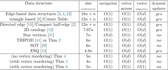
Data structure size navigation vertex vertex dynamic

(references) access adjacency updates Edge-based data structures [3,4,24] 18n + n O(1) O(1) O(d) yes

triangle based [8]/Corner Table 12n + n O(1) O(1) O(d) yes Directed edge [10]/Compact half-edge [2] 12n + n O(1) O(1) O(d) yes 2D catalogs [12] 7.67n O(1) O(1) O(d) yes Star vertices [31] 7n O(d) O(1) O(d) no TRIPOD [41] or Thm2 6n O(1) O(d) O(d) no

SOT [29] 6n O(1) O(d) O(d) no

ESQ [13] 4.8n O(1) O(d) O(d) yes

(no vertex reordering) Thm 4 5n O(1) O(d) O(d) no (with vertex reordering) Thm 5 4n O(1) O(d) O(d) no (with vertex reordering) Thm 6 5n O(1) O(1) O(1) no

Table 1: Comparison between existing data structures for triangle meshes. All storage and runtime bounds hold in the worst case. The degree of the accessed vertex is denoted d. Storage costs are expressed in terms of the number n of vertices.

in main memory during the pre-processing construction phase. This issue is addressed by Grouper [35]: the combination of compact mesh data structures with techniques from streaming meshes for out-of-core computations allows constructing the compact represen-tation on the fly from a compressed format and in a streamable way.

Finally, we observe that the parsimonious use of references may affect the navigation time, for the retrieval of some mesh elements: for example, the access to vertices may require more than O(1) time in the worst case [13,26,29,31]. Table1reports some trade-offs between space requirements and navigation performance.

Theoretically optimal solutions. For completeness, we mention that succinct represen-tations [7,15,16,18,37,43] are successful in representing meshes with the minimum number of bits, while supporting local navigation in worst case O(1) time. They run under the word-Ram model, where basic arithmetic and bitwise operations on words of size O(lg n) are performed in O(1) time. One main idea (underlying almost all solutions) is to reduce the size, and not only the number, of references: one may use graph separators or hier-archical graph decomposition techniques in order to store in a memory word an arbitrary (small) number of tiny references. Typically, one may store up to O(_{lg lg n}lg n ) sub-words of length O(lg lg n) each. Unfortunately, the number of auxiliary bits needed by the encoding becomes asymptotically negligible only for very huge graphs, which makes succinct repre-sentations of mainly theoretical interest.

For a more detailed discussion on triangle mesh data structures we refer to [14], while a comprehensive explanation of recent advances in 3D mesh compression can be found in [1,36].

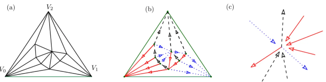
V0 V1

V2

(a) _(b) (c)

Figure 1: A planar triangulation with 9 vertices (a), endowed with a Schnyder wood (b). Picture (c) local Schnyder condition around inner vertices.

1.3 Preliminaries

Combinatorial aspects of triangulations. In this work we exploit a deep and strong combinatorial characterization of planar triangulations. A planar triangulation is a sim-ple planar map where every face has degree 3.2 Triangulations are rooted if there is one distinguished root face, denoted by (Vred, Vblue, Vblack), with a distinguished incident root

edge {Vred, Vblue}. Inner edges (and inner vertices) are those not belonging to the root face

(Vred, Vblue, Vblack).

As pointed out by Schnyder [40], the inner edges of a planar triangulation can be partitioned into three sets Tred, Tblue, Tblack, which are plane trees spanning all inner vertices,

and rooted at Vred, Vblue and Vblack respectively. This spanning condition can be derived

from a local condition. The inner edges can be oriented in such a way that every inner vertex is incident to exactly 3 outgoing edges, and the orientation/coloration of edges must satisfy a special local rule (see Figure 1).

Definition 1 ( [40]). Let G be a planar triangulation with root face (Vred, Vblue, Vblack).

A Schnyder wood of G is an orientation and labeling, with label in {red,blue, black} of the inner edges such that the inner edges incident to the vertices Vred, Vblue, Vblack are all

incoming and are respectively of color red, blue, and black. Moreover, each inner vertex v has exactly three outgoing incident edges, one for each color, and the edges incident to v in counter clockwise (ccw) order are:

one outgoing edge coloredred,

zero or more incoming edges colored black, one outgoing edge coloredblue,

zero or more incoming edges colored red, one outgoing edge colored black, and zero or more incoming edges colored blue

(this is referred to as local Schnyder condition).

In a triangulation, the edges are originally not oriented, and they get an orientation during the Schnyder wood construction. If an edge e between vertices u and v is oriented

2

from u to v, it will be denoted (u, v) and (v, u) if the edge is oriented in the other direction. If the orientation is unknown the edge will be denoted by {u, v}. In a Schnyder wood, the inner edges get an orientation, thus we have either {u, v} = (u, v) or {u, v} = (v, u).If (u, v) is an edge of color c, we say that v is the parent of u in Tc. The two oriented edges (u, v)

and (v, u) never exist together (a simple triangulation does not contain multiple edges). A Schnyder wood of a planar triangulation [40] can be computed in linear time: for the sake of completeness we provide in Appendix A a short illustration of the algorithm based on vertex conquests detailed in [9,33].

Navigational operators.

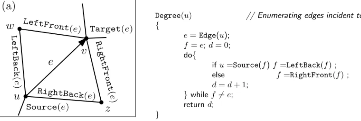
Here are the operators supported by our representations. Let e = (u, v) be an edge oriented toward v, which is incident to (u, v, w) (its left triangle) and to (v, u, z) (its right triangle), as depicted in Figure2.

• LeftBack(e) returns the edge {u, w} (i.e. (u, w) or (w, u)). • LeftFront(e) returns the edge {v, w}.

• RightBack(e) returns the edge {u, z}. • RightFront(e) returns the edge {v, z}. • Source(e) returns u.

• Target(e) returns v.

• Edge(u) returns an edge outgoing from vertex u;

• Point(u) returns the geometric coordinates of vertex u. • Edge(f ) returns an edge incident to face f ;

• Faceleft(e) returns the face at the left of oriented edge e;

RightFront (e₎

e

u

z

v

w

(a)

Degree(u) // Enumerating edges incident to u . { e = Edge(u); f = e; d = 0; do{ if u =Source(f ) f =LeftBack(f ) ; else f =RightFront(f ) ; d = d + 1; } while f 6= e; return d; }

Figure 2: (a) Navigational operators supported by our representations.

• Faceright(e) returns the face at the right of oriented edge e;

The operators above are supported by most mesh representations [3,10], and allow full navigation in the mesh as required in geometric processing algorithms. Their combina-tion allows us to walk around the edges incident to a given face, or to iterate on the edges incident to a given vertex leading, for instance, to support the operator

• Adjacent(u, v), test whether two vertices u and v are adjacent.

This last operator cannot be supported in constant worst case time by common mesh representations: testing the adjacency between vertices is sometimes needed in graph algorithms, and the timing cost is proportional to the degree of the involved vertices.

Overview of our Solution In order to design new compact array-based data structures, we make use of many ingredients: some of them concerning the combinatorics of graphs, and some of them pertaining the design of compact (explicit) data structures. The main steps of our approach are the following:

• as done in [41], we exploit the existence of 3-orientations (edge orientations where every inner vertex has outgoing degree 3) for planar triangulations [40]. This allows storing only two references per edge (corresponding to its LeftFront and RightFront edges).

• as done in [10,26,29], we perform a reordering of cells (edges), to implicitly represent the map from vertices to edges, and the map from edges to vertices;

Combining these two ideas one can easily obtain an array-based representation using 6n references: we store the three edges outgoing from a vertex consecutively, so that the retrieval of the missing information involving the LeftBack and RightBack edges can be efficiently performed by exploiting the local Schnyder condition. Our first data structure provides O(1) time navigation between edges and O(d) time for the access to a vertex of degree d: for the sake of completeness, this simple solution will be detailed in Theorem 2.

Additionally, we design a coding scheme that can produce a compressed file of size 4n bits which is just above the theoretical lower bound of 3.24 bits per vertex [38]); our array-based representation can be restored from the compressed file without using extra memory. Our main contribution is to show how to get further improvements and generalizations, using the following ideas:

• we exploit the existence of maximal Schnyder woods. A Schnyder wood is maximal if it does not contain any oriented cycle of edges oriented in clockwise direction 3_{. We}

also exploit the fact that, given the partition (Tred, Tblue, Tblack), the two trees Tred and Tblack, are sufficient to retrieve the triangulation. With these ideas we succeed to

store only 5n references (Theorem4). 3

Given an edge orientation of a triangulation G endowed by a Schnyder wood, we say that a cycle of edges is an oriented cycle if all its edges are oriented in the same (clockwise or counterclockwise) direction.

• we show how to reconstruct our compact representations (Theorems 4 and 2) from a compressed format that uses less than 4n bits, without extra memory: both the encoding and decoding phases require linear time (Section 3).

• we further push the limits of the previous reordering approach: by arranging the vertices according to a given permutation and using a special order on plane trees we are able to use only 4n references (Theorem5);

• Using one extra reference per vertex, we are able to efficiently recover the target of every edge, providing worst case O(1) time access to vertices instead of O(d) (Theo-rem 6).

• Our compact data structure described in Theorem 6 supports even the Adjacent operator in O(1) time on planar triangulations.

• For applications requiring to store data associated with triangles, Theorem 7 shows how to represent the map between edges and triangles using one additional reference per vertex (the retrieval of data associated with triangles is performed in O(1) time). Storing data associated with corners (representing incidence relations between vertices and faces) can be done without extra references.

To our knowledge, these are the best (worst case and guaranteed) upper bounds obtained so far, which improve previous results. Finally we mention that our representations can be adapted to deal with more general triangle meshes, by using the reformulations of Schnyder woods proposed for toroidal [20,22] and genus g [17] triangulations.

2 Compactly Representing Triangulations

We first design a simple data structure requiring 6n references, which allows performing all navigational operators in worst case O(1) time, and Target operator in O(d) time (when retrieving a degree d vertex). This is a preliminary step in describing a more compact solution. Observe that our first scheme achieves the same space bounds as the Tripod data structure by Snoeyink and Speckmann [41]. Although both solutions are based on the properties of Schnyder woods, the use of references (between edges) is different: this is one of the features which allow us to make our scheme even more compact in the sequel.

2.1 The First Data Structure: Simple and Still Redundant

Main ideas: the coloring of edges allow an easy matching between vertices and edges of each color to organize edges in three arrays. For each edge we store the leftfront and rightfront edges; the leftback and the rightback edges are retrieved using Schnyder wood rules.

Scheme Description. We firstly compute a Schnyder wood (Tred, TblueTblack) of the input

(Vblue, Vred) and (Vblack, Vred) to Tred; we add the edge (Vblack, Vblue) to the tree Tblue, as

depicted in Figure 3. Thus each edge gets a color and an orientation. Since local Schnyder condition ensures exactly one outgoing edge of each color (except Vred, Vblue, Vblack) an edge

can also be identified by its origin u and its color c and denoted u%

c. For each color c and

each vertex u, we store two vertex indices Sleft_c [u] and S_cright[u] and two booleans C_cleft[u] and C_cright[u] describing the source and color of the two neighboring edges of edge u%

c as

detailed below and one boolean Ic[u] indicating the existence of incoming edge at u of color

c.

Vertices will be identified by integers 0 ≤ i < n and edges by their source and color. The three colors are cyclically ordered with operator next and prev such that next(red) =

blue, next(blue) = black, and next(black) = red. Our data structure consists of several arrays of size n:

- three arrays of booleans Ired, Iblue, and Iblack (I standing for incoming),

- six arrays of booleans C_redleft, C_redright, C_blueleft, C_blueright, C_blackleft , C_blackright (C standing for color), - six arrays of vertex indices S_redleft, S_redright, S_blueleft, S_blueright, S_blackleft , S_blackright (S standing for source), - an array P storing the geometric coordinates of the points.

These arrays store the following information (refer to Figure 3) for a vertex u and a color c (the three vertices of the outer face do not have all their outgoing edges and must obey special rules):

Ic[u] = true if vertex u has at least one incoming edge of color c, false otherwise,

S_cleft[u] = Source(LeftFront(u%

c)), and Scright[u] = Source(RightFront(u

%

c)),

Using the coloring rules, these two neighboring edges have only two possible colors: c and next(c) (resp. prev(c)) for a left neighbor (resp. right neighbor). Arrays Cc store that

information:

if Color(LeftFront(u%

c)) = c then Ccleft[u] = true, else Ccleft[u] = false,

if Color(RightFront(u%

c)) = c then Ccright[u] = true, else Ccright[u] = false.

Theorem 2. Let G be a triangulation with n vertices. The representation described above requires 6n references, while allowing support of Target operator in O(d) time (when dealing with a degree d vertex) and all other operators in O(1) worst case time.

Proof. Let us consider operations involving an edge e with source u and target v, whose incident left (resp. right) triangle is (u, v, w) (resp. (v, u, z)).

Operators Edge(u) and Point(u): to get the index of an edge incident to a given vertex u we simply returns the edge u%

red. The geometric coordinates of vertex u are naturally stored in P [u].

Operator LeftFront(e): by definition of arrays S and C, LeftFront(e) is the edge of source S_Color(e)left [Source(e)] and color Color(e) if C_Color(e)left [Source(e)] = true and color next(Color(e)) otherwise.

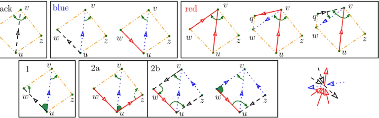
Operator LeftBack(e): We have to distinguish three cases, depending on the color of edges (u, w) and (v, w) (as illustrated in Figure3):

Case 1: I_{prev(Color(e))}[Source(e)] is false. This case is easy to handle, since (u, w) is the edge with source u and color next(Color(e)) (in Figure3(c), there is no incomingblue

edge at u, thus LeftBack(e) is redand outgoing at u).

Case 2: I_{prev(Color(e))}[Source(e)] is true and C_Color(e)left [Source(e)] is true. Then (w, v) is of color Color(e) and (v, w) can be accessed as LeftFront(e) and LeftBack(e) is the edge with source Source(LeftFront(e)) and color prev(Color(e)) (there are incoming

blueedge at u, thus LeftBack(e) isblue. Since LeftFront(e) = {v, w} is black, it is oriented from w to v and its source is also the searched source of LeftBack(e)).

Case 3: Iprev(Color(e))[Source(e)] is true and CColor(e)left [Source(e)] is false, then (v, w)

is of color next(Color(e)) and LeftBack(e) is the edge LeftFront(LeftFront(e)). (as in Case 2 LeftBack(e) is blue, but LeftFront(e) = {v, w} is red and oriented from v to w. LeftBack(e) is then accessible as LeftFront(LeftFront(e)) ).

Operator Target(e): unfortunately we have not stored enough information to return v in O(1) time: the idea is to iteratively turn around vertex v (as described in Figure2), starting from edge (u, v) in cw direction (or ccw direction) until we get an edge e0 = (v, x) having v as source. Then compute Source(e0) in O(1) time as above, which results in the target of (u, v). This procedures ends after at most d − 3 steps (for a vertex v of degree d), since each vertex has 3 outgoing edges.

Operators RightBack(e) and RightFront(e): observe that the traversal of the right face (u, v, z) incident to (u, v) can be handled in a similar manner as above.

Operators RightBack(e) and RightFront(e) can be deduced by symmetry from operators LeftBack(e) and LeftFront(e), because of the symmetry of Schnyder woods and of our use of reference.

References Encoding. From a practical point of view, arrays I, C and S can be stored in a single array. Just encode the service bits within the references stored in srcf ront, where first k bits of an integer represent the index of a vertex, and the booleans in the other bits of an integer. We can set k = dlog ne. We use only less than 2 service bits per integer since we have 9 service bits to associate with 6 vertex indices. Assuming 32-bit integers, we can encode triangulations having up to 230 (1 billion) vertices in 6 arrays of n integers.

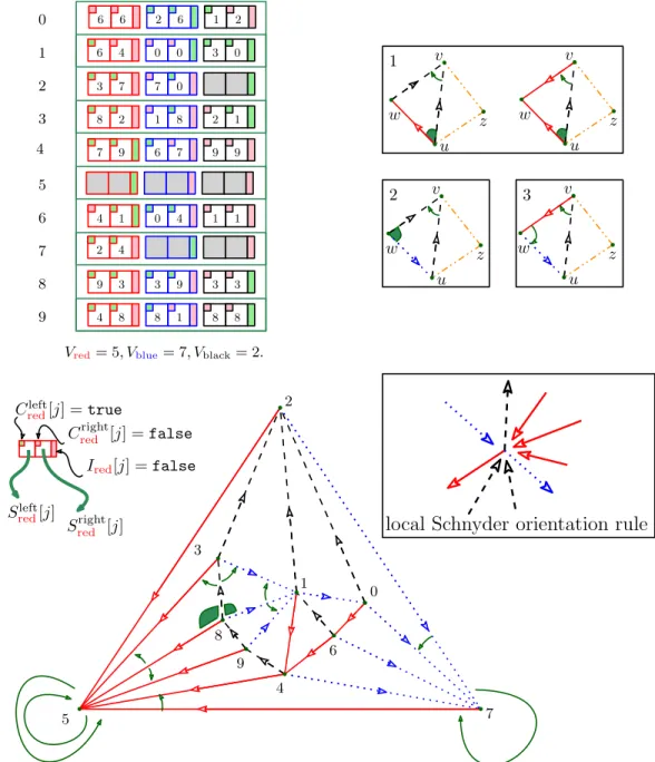
z w w _z z w w _z u v u v u v u v 1 2 3 3 4 5 6 7 8 9 0 1 2 Vred= 5, Vblue= 7, Vblack= 2.

local Schnyder orientation rule

C_redleft[j] = true

C_redright[j] = false

S_redright[j] Ired[j] = false Sleft red[j] 6 7 8 9 0 1 2 3 5 4 7 6 8 9 0 1 2 3 4 6 7 8 9 0 1 2 3 9 7 8 0 9 2 3 4 6 7 8 9 0 1 2 3 4 6 6 0 8 1 2 3 4 8 1 3 4 1 1

Figure 3: Our first solution. For each vertex we store 6 references, corresponding to the source of the front neighbors of the 3 outgoing edges. Tables I, C, S are drawn as an array of size n where booleans are represented by colors (green=true, pink=false). The interpretation of the figure is as follows: vertex 8 has no red incoming edges thus Ired[8] is false (pink), the left front edge of the red edge outgoing Vertex 8: 8%

red = (8, 5) is (9, 5) = 9%

red thus the first box of line 8 of the array is green (same color) and contains 9. The case analysis of Theorem 2is illustrated on the top right (when edge (u, v) is black).

2.2 More Compact Solutions, via Maximal Schnyder Woods

Main idea: modify previous scheme to store only one of the two (leftfront and rightfront) neighbors for the blue edges. Again use Schnyder woods properties to retrieve missing information.

In order to reduce the space requirements, we exploit the existence of a special kind of Schnyder wood, called maximal, not containing cw oriented cycles, and in particular no oriented cw triangles. For example in Figure 3 the Schnyder wood is not maximal because (1, 4, 9) is a cw oriented cycle, while in Figure 5 the Schnyder wood is maximal because there is no cw oriented triangle (but there is a ccw oriented triangle (2, 3, 7)). This property can be used to prove that some cases cannot occur and allows us to avoid to store some pieces of information.

Lemma 3 ( [9]). Let G be a planar triangulation. Then it is possible to compute in linear time a Schnyder wood without cw oriented cycles of directed edges.

New Scheme. We modify the representation described in previous section: the first step is to endow G with its maximal Schnyder wood (no cw oriented triangles). Outgoing red and black edges will be still represented with two references each, while we will store only one reference for each outgoing blue edge (different cases are illustrated by Figure 4, top pictures). More precisely, let e = (u, v) be an edge having face (u, v, w) at its left and face (v, u, z) at its right, and let q be the vertex defining the ccw triangle (w, v, q). Our data structure still consists of several arrays of size n:

- three arrays of booleans Ired, Iblue, and Iblack,

- four arrays of booleans C_redright, Cblue, Cblackleft , C right black

- one array of colors C_redtoleft that can take three values: {red,blue, black}. - five arrays of vertex indices S_redtoleft, S_redright, Sblue, Sblackleft , S

right black, and

- an array P storing the geometric coordinates of the points.

With respect to the simple solution arrays C_blueleft, C_blueright, S_blueleft, S_blueright, S_redleft, and C_redleft are replaced by Cblue, Sblue, Sredtoleft, and Credtoleft with slightly different content and meaning. This change is emphasized by the the slight change of names from left to toleft. In the previous scheme, Tables Cc are storing a boolean representing whether the color of the left

front (and right front) edges coincide with the color of the current edge (u, v). In the new scheme, and just for the neighbor of the red edge to the left, the color can be any of the three colors so we store directly this color. Roughly, only one neighbor of the blueedge is stored, and for therededge, we may store the second left neighbor (the second edge turning cw around the target) instead of the first one. For a vertex u the following entries have the

same meaning as in the previous solution:

Ic[u] = true if vertex u has incoming edges of color c, false otherwise,

S_redright[u] = Source(RightFront(u%

red)), S_blackleft [u] = Source(LeftFront(u%

black)), and S right

black[u] = Source(RightFront(u

%

black)),

if Color(RightFront(u%

red)) =red then C

right

red [u] = true, else C

right

red [u] = false, if Color(LeftFront(u%

black)) = black then Cblackleft [u] = true, else Cblackleft [u] = false,

if Color(RightFront(u%

black)) = black then C right

black[u] = true, else C right

black[u] = false.

Some other entries are modified with respect to the simple version. If (u, v) is ablue

edge then we store only one of the two neighbors. The choice of the neighbor that is stored depends on the existence ofred edges incoming at u:

if Ired[u] then

Sblue[u] = Source(LeftFront(u%_blue))

if Color(LeftFront(u%

blue)) =blue then Cblue[u] = true, else Cblue[u] = false,

else

Sblue[u] = Source(RightFront(u%blue)),

if Color(RightFront(u%

blue)) =blue then Cblue[u] = true, else Cblue[u] = false,

If {u, v} is a red edge, we store its second left neighbor in place of the first one when this second neighbor is black. Otherwise we store its first neighbor, as previously, and this neighbor can be redorblue. It yields a total of three cases distinguished by the three possible values of C_redtoleft (see Figure4-top-right).

if {w, v} is redthen C_redtoleft[u] =redand S_redtoleft[u] = w, if {w, v} isblue and {v, q} is redthen C_redtoleft[u] =blueand S_redtoleft[u] = v, if {w, v} isblueand {v, q} is black then C_redtoleft[u] = black and S_redtoleft[u] = q,

Theorem 4. Let G be a triangulation with n vertices. There exists a representation requir-ing 5n references, allowrequir-ing efficient navigation, as in Theorem 2.

Proof. We just need to explain how to retrieve the missing RightFront or LeftFront information. The other operations can be obtained as in the proof of Theorem 2.

We consider an edge e from u to v with incident triangles (v, u, z) on the right and (u, v, w) on the left. We first assume that e is an inner edge (the case of exterior edges is described below).

• If e is black (Figure4-top-left),

both RightFront(e) and LeftFront(e) are directly stored. • If e is red(Figure4-top-right),

RightFront(e) is directly stored. LeftFront(e) is either directly stored if C_redtoleft 6= black or accessible using RightFront(e0), where e0 = (q, v) is stored, otherwise.

z w u v blue z w u v black z w u v 2b 2a z w u v z w u v 1 q z w u v red z w u v q z w u v z w u v z w u v

Figure 4: More compact scheme. Neighboring relations between edges are represented by tiny oriented (green) arcs corresponding to stored references, and by filled (green) corners that implicitly describe adjacency relations between outgoing edges incident to the same vertex: because of local Schnyder rule, we do not need to store references between neigh-boring outgoing edges.

• If e is blue(Figure4-top-middle),

one of RightFront(e) or LeftFront(e) is directly stored and the other can be retrieved as follows:

Case 1 {u, w} is black (if Ired[u] =false, Figure4-bottom-1)

and thus towards w, then RightFront(e) is directly stored and LeftFront(e) is given by computing RightFront(u%

black).

Case 2 {u, w} isred(if Ired[u] =true, Figure 4-bottom-2a and 2b) and thus towards u, then LeftFront(e) is directly stored.

Case 2a {u, z} isred (if Iblack[u] =false, Figure4-bottom-2a)

and thus towards z, then RightFront(e) can be retrieved as LeftFront(u%

red). Case 2b {u, z} is black (if Iblack[u] =true, Figure4-bottom-2b)

and thus towards u: since clockwise oriented triangles are forbidden, {z, v} is necessar-ily towards v and thus blue. Edge {v, w} can be either black or blue, and is accessi-ble as LeftFront(e). Vertex w can be accessed as Source(LeftFront(LeftFront(e))) if LeftFront(e) is black (Figure 4-bottom-2b-left), and as Source(LeftFront(e)) otherwise (Figure 4-bottom-2b-right). Then, we are in the special case where (w, u) = w%

red stores a reference to z, the source of the second left edge, and {z, v} is now accessed as z%

blue.

Observe that it is possible to distinguish between cases in O(1) time just reading the I and C arrays.

The case of an exterior edge (u, v) incident to the outer face is dealt with as follows. If e = (Vblue, Vred) or e = (Vblack, Vred) then the navigation operators are performed as in Thm 2. If e = (Vblack, Vblue) then RightFront and RightBack are performed as described

above for the case of inner edges: observe that the result of RightFront(u%

blue) is stored by

construction in Sblue[u]. Finally, the two remaining cases are dealt with in a special manner:

the LeftFront and LeftBack operators are defined to return v%

redand u

%

2.3 Further Reducing the Space Requirement

Main idea: order the vertices according to theredtree such that some leftfront or right-front neighbors for therededges can be found using arithmetic operations instead storing references. Schnyder woods properties are still used to retrieve missing information.

Allowing the exploitation of a permutation of the input vertices (reordering the vertices according to a given permutation), we are able to save one more reference per vertex. In particular, we need an ordering such that the vertices having the same parent vertex u in Tred, will have consecutive numbers (when traversed turning cw around u from u%

black): a simple breadth-first search traversal of Tredcomputes such an ordering (denoted

cwBFS ). Another possible choice could be the DFUDS ordering used in [5].

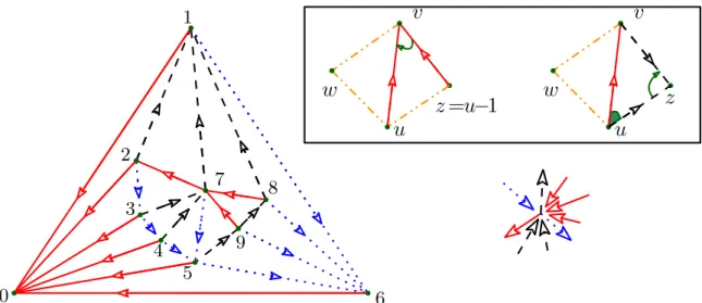
Scheme description. We first compute a maximal Schnyder wood of G, and perform the cwBFS traversal of Tred starting from its root Vred: as Tred is a spanning tree of all vertices of G, we obtain a vertex labeling such that, for every vertex v ∈ G, the children of v in Tred have consecutive labels (as illustrated in Figure 5). We then reorder all vertices (their associated data) according to their cwBFS label, and we store entries in table C accordingly. This allows us to save one reference per vertex: we do not store a reference to RightFront for edges in Tred, which leads us to not store tables Credright and S

right

red , and retrieve the corresponding information using the ordering of vertices as explained below. All other tables are exactly as in the previous section. We can state the following result (the case analysis is partially illustrated by pictures in Figure 5):

Theorem 5. Let G be a triangulation with n vertices. If one is allowed permuting the input vertices (their associated geometric data) then G can be represented using 4n references, supporting navigation as in previous representations.

Proof. Compared to the representation of Theorem 4 we lose the information concerning RightFront for rededges (which was previously explicitly stored in C_redright and S_redright). An important remark is that, given a rededge e = (u, v), we retrieve its right siblings in T_red just using its cwBFS label.

More precisely, RightFront(u%

red) is either red or black. If it isred, then it is (u − 1)%

red. It is possible to decide if this is the case by checking if u

%

red= LeftFront((u − 1)

%

red). In the other case, edge {u, z} must also be black because clockwise oriented triangles are forbidden, and thus RightFront(u%

red) can be obtained as LeftFront(u

%

black).

2.4 All Operations in O(1) Worst Case Time

We can further exploit the redundancy in our representation in order to improve the computational cost of the navigation: both Target and Adjacent operators can be supported in worst case constant time. The solution relies on a very simple idea: we add a new table storing explicitly a reference to the target vertex of u%

blue or u

%

black. We also use

a service bit to store the parity of the depth of a given vertex in theredtree, and we store the target of u%

3 4 5 6 7 ₈ 9 0 1 2

z =u−1

w

u

v

z

w

u

v

Figure 5: A planar triangulation (endowed with its maximal Schnyder wood) whose vertices are labeled according to the cwBFS traversal of tree Tred (right). On the right are shown all cases involved in the proof of Theorem5: we now store only one reference forrededges, since most adjacency relations between edges inTredare implicitly described by the cwBFS labels.

be retrieved by other means. More precisely, we have the following theorem:

Theorem 6. If one is allowed permuting input points, then there exists a compact repre-sentation requiring 5n references which supports all navigation operators (including Target and Adjacent) in worst case O(1) time.

Proof. The data structure of Theorem5 is modified and extended as follows: — S_redleft[u] stores Target(u%

red). Notice that when LeftFront(u%

red) is red, Source(LeftFront(u

%

red)) and Target(u

%

red) are the same and the content of S_redleft[u] is the same as before.

— A new Boolean array D (standing for depth parity) is created with D[u] = true if u has even depth in the redtree, D[u] = false otherwise.

— A new array W storing vertex indices is created. If Ired[u] = false (that is u is a leaf of theredtree), then W [u] = Target(u%

Color(LeftFront(u%_blue))).

If Ired[u] = true (u is not a leaf), then W [u] = Target(u%c), where c = black if D[u] = true

(the depth of u in the redtree is even), and c =blueotherwise.

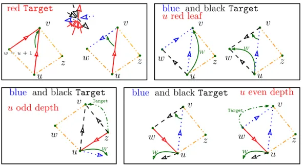
Target operator. We now explain how the Target operator can be implemented for each color, and how the LeftFront operator is modified for red edges (see Figure6); the imple-mentations of the other operators remain unchanged.

— LeftFront(u%

red):

If C_redleft[u] = true then LeftFront(u%

red) is (u + 1)

%

red else LeftFront(u%

red) is stored in Sredleft[u]. — Target(u%

W

u

z

v

red Target

z

w

u

v

u red leaf

z

w

u

v

z

w

u

v

u

z

w

u

v

u even depth

z

w

u

v

blue

and black Target

blue

and black Target

z

w

v

u odd depth

Target

blue

and black Target

Figure 6: Illustration of case analysis of Theorem6: the Target operator can be performed in O(1) time using 5n references.

— Target(u%

blue).

If Ired[u] = false and Cblueleft[u] = true, the result is directly stored in W [u].

If Ired[u] = false and Cblueleft[u] = false, the result is Source(LeftFront(u

%

blue)).

If Ired[u] = true and D[u] = false, the result is directly stored in W [u]. If Ired[u] = true and D[u] = true and Cblueleft[u] = false,

the result is Source(LeftFront(u%

blue)).

If Ired[u] = true and D[u] = true and Cblueleft[u] = true,

the result is Target(LeftFront(u%

blue)).

Notice that at the last line, we need the Target of a blue edge whose source w has odd depth: the result is thus directly stored in W if w is not a leaf of the red tree or computable otherwise.

— Target(u%

black) implementation is similar to the one of Target(u

%

blue), up to one forbidden

case since there is no cw triangle:

If Ired[u] = false and Cblueleft[u] = false, the result is directly stored in W [u].

If Ired[u] = false and Cblueleft[u] = true, the result is Source(LeftFront(u

%

blue)).

If Ired[u] = true and D[u] = true, the result is directly stored in W [u]. If Ired[u] = true and D[u] = false, the result is Target(RightFront(u%black)).

Adjacent operator. The constant time cost of Target directly leads to a very simple and O(1) time implementation of the Adjacent(u, v) operator. We first get the three target vertices of the 3 edges outgoing from u. These three neighbors of u are retrieved by computing Target(u%

black), Target(u

%

blue) and Target(u

%

red): we check whether one of them does coincide with vertex v. Similarly, we retrieve three neighbors of vertex v by computing Target(v%

black), Target(v

%

blue) and Target(v

%

does coincide with vertex u.

Since in a triangulation endowed with a Schnyder wood each (inner) vertex has outdegree 3, we know that there exists an edge {u, v} if and only if one of the 6 tests described above returns a positive answer.

2.5 Representing Faces

One limitation of the encoding schemes presented at the previous sections concerns the fact that our data structures are edge-based and do not allow us to explicitly represent the triangle faces: this could be a desirable requirement for some geometric processing applications.

In some situation, various kinds of data related to triangles need to be stored (such as face colors, face normals, . . .): for this purpose common mesh data structures store, in addition to the incidence relations between edges and vertices, the map between faces and edges. For instance, common implementations of the half-edge data structure [32] store for each half-edge a reference to the incident face, and for each face they store a reference toward one incident half-edge: this requires (2 + 6)n = 8n references that must be added to the 19n references of the basic implementation of the half-edge data structure.

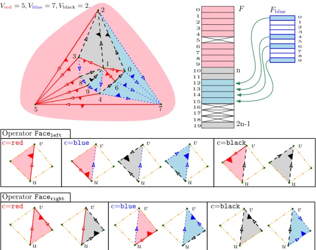
In the case of our compact data structures we can represent the map between faces and edges in a more concise way, exploiting again the structural properties of Schnyder woods. In order to construct the mapping from edges to triangles, we first endow the triangulation with its maximal Schnyder wood. Then we match some edges with the triangle that lies at their left. Observe that, since there are no cw oriented cycles of directed edges, each triangle is at the left to at least one edge.

First, we match all (n − 1) red edges with the triangles at their left and call these triangles “red triangles” (see Fig.7). Second, we match the black edges having a non-red triangle at their left with their left face: these are called “black triangles”. Finally, the remaining triangles are called “bluetriangles and must be at the left of one blueedge, and are matched with thisblue edge.

The idea is to index the triangles using numbers from 0 to 2n − 1 in the following way: (i) The triangles matched with arededge get the index of the source of the rededge (all red edges are matched with a triangle). Observe that each red triangle is matched to exactly one red edge: the local property of Schnyder woods ensures that in a triangle incident to two red edges both edges must be oriented toward the same vertex. (ii) The triangles matched with a black edge get the index of the source of the black edge plus n (some black edges remain unmatched) (iii) The triangles matched with a blueedge get the index of the source of an unmatched black edge that must be stored in some auxiliary table Fblue described in the proof of the following theorem:

Theorem 7. The data structures of Theorems 2, 4, and 5 can be extended to store infor-mation in triangles using one additional reference per vertex. Access to the inforinfor-mation is done in O(1) time.

Proof. A triangle of color c is represented by its corresponding edge u%

match-Vred= 5, Vblue= 7, Vblack= 2. u v u v c=red u v c=blue u v c=black u v u v Operator Faceright

c=red c=blue c=black

Operator Faceleft

u v u v u v u v u v u v 3 4 5 6 7 8 9 0 1 2 Fblue 6 7 8 9 0 1 2 3 5 4 10 11 12 13 14 15 F 16 17 n 2n-1 18 19 6 7 8 9 0 1 2 3 5 4

Figure 7: Mapping from edges to triangles (indicated by small triangles). Bottom pictures illustrate the case analysis of Theorem7.

ing and denoted u∆

c. In addition to the input data associated with faces (e.g. face colors or

normals), we make use of an additional array that represents the mapping fromblue edges tobluetriangles. More precisely, we have:

- one array of size n of face indices Fblue (standing for face indirection) and

- one array of size 2n of face information F (standing for face information). Four entries in F are unused.

The information stored in the array F can be retrieved with the following rules: data associated with u∆

redare stored in I[u] data associated with u∆

black are stored in I[n + u]

data associated with u∆

blue are stored in I[n + Fblue[u]]

We now explain how to retrieve the indices of the two faces incident to a given edge (Faceleft and Facerightoperators, see Figure 7).

Faceleft operator The Faceleft operator can be implemented as follows for an edge u%c: — If c =red Faceleft(u % red) is u ∆ red — If c = black

If LeftFront(u) isredthen Faceleft(u

%

black) is given by Source(LeftFront(u))

∆

red else Faceleft(u

%

black) is u

∆

black

— If c =blue

If LeftBack(u) isred then Faceleft(u

%

blue) is Source(LeftBack(u))

∆

red

else If LeftFront(u) is black then Faceleft(u%_blue) is Source(LeftFront(u))∆_black

else Faceleft(u

%

blue) is simply u∆blue

Faceright operator The Facerightoperator can be implemented as follows for an edge u%c:

— If c =red

If RightFront(u) is redthen Faceright(u%_red) is Source(RightFront(u))∆_red

else Faceright(u

%

red) is u∆black (recall that cw oriented triangles are forbidden).

— If c = black

If RightFront(u) is black then Faceright(u%_black) is Source(RightFront(u))∆_black

else Faceright(u

%

black) is Source(RightBack(u))∆blue

— If c =blue

If RightBack(u) is redthen Faceright(u%_blue) is Source(RightBack(u))∆_red

else Faceright(u

%

blue) is Source(RightFront(u))

∆

blue

Finally, observe that the two operators above can be performed in worst case O(1) time since their implementation does not involve the Target operator.

Edge operator The Edge operator for a face u∆

c trivially returns u%c.

To initialize Fblue we need an extra array of booleans A (standing for available

entry) of size n. The array A is only temporarily used and not necessarily required: its information could be stored in the array F , since F is not yet initialized at that step. Array A is initialized at true at the beginning. Then in a first step: for each black edge u%

black if

Faceleft(u

%

black) = u

∆

black we set A[u] = false. In a second step: for each blue edge u

%

blue

we set Fblue[u] = v such that A[v] = true and we set A[v] = false.

Notice that if storing information in faces is not needed, it is still possible to design a procedure to iterate over all faces in constant time per face without using additional storage. A simple solution consists in performing a DFS traversal of the dual graph, avoiding to traverse the edges of theredtree: this is similar to the traversal performed to compute the binary encoding string that will be described in Section3.1.

2.6 Representing Corners

In some cases, we needed to attach information to corners, i.e. to an incidence between a vertex v and a triangle t. Actually we associate a corner (v, t) to the edge e following v in t in ccw order. In this way an edge is associated to two corners, one in each incident triangle.

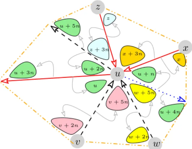
u v _w x z u u + n u + 2n x + 3n z + 3n v + 5n w + 5n z w + 2n x v + 2n u + 3n u + 5n u + 4n

Figure 8: Mapping from edges to corners (Theorem 8).

The green corners are the 6 corners associated to the three edges with source u.

Actually, according to the orientation given to an edge by the Schnyder wood, an edge is associated with the incidence between its source and its left face and the incidence between its target and its right face.

Theorem 8. The data structures of Theorems 2, 4, and 5 can be extended to store infor-mation in corners using no additional reference per vertex. Access to the inforinfor-mation is done in O(1) time.

Proof. Looking at a corner around a vertex, one can observe that there is a natural bijection between the incident edges and the corners of that vertex: just associate an edge with the corner just after it counterclockwise around the vertex (see Figure 8). Then the corners are numbered from 0 to 6n − 1 and mapped to their corresponding incident edges with the following rule.

Let us consider a corner incident to a vertex u and mapped to an incident edge e. If u is the source of e, then the index of the corner will be u, u + n or u + 2n depending on whether the edge e is respectively red,blue, or black. Otherwise the vertex u is the target of e, and the index of the corner will be u + 3n, u + 4n or u + 5n respectively forred,blue

or black edges.

3 Decoding the Triangulation from a Compressed Format

A main issue common to many compact data structures [12,13,26,27,29], is that an explicit representation of the entire mesh must be kept in main memory during the whole construc-tion phase: this is needed, for example, to process vertices and edges (or faces), which must be re-numbered according to a prescribed mesh traversal. This preliminary construction phase can greatly increase the overall memory requirements, especially for very huge meshes: in addition to the space storage of the compact data structure to construct (between 4n

and 8n references for most compact representations), one has to use between 13n and 19n references for an explicit representation (such as Corner Table or Half-edge), and a few additional memory references for the implementation of the mesh processing (typically, a graph traversal). To address this issue, one could take advantage of the existence of various and efficient compressed formats for triangle meshes, which have been designed in order to store a triangulation on disk or to send it on the network.

In this section we show how to save our array-based compact representations in a compressed format so that we can reconstruct on the fly our structure in linear time, without any extra memory cost and in a streamable fashion. The first construction of our representation still needs an explicit representation, in particular for the computation of the Schnyder wood. This format allows coding/decoding a planar triangulation of n vertices with less than 4n bits. The encoding scheme, originally designed for the planar case [30], relies on the combinatorial properties of Schnyder woods (or the related canonical orderings structure) and provides a bijection between the set of all Schnyder woods of a given planar triangulation and pair of non-crossing Dyck paths [6]. More recently this scheme has been generalized for dealing with genus g triangulations [17].

3.1 Encoding Scheme

For the sake of completeness, we provide a concise overview of the encoding scheme for planar triangulations (a more detailed presentation can be found in [6]).

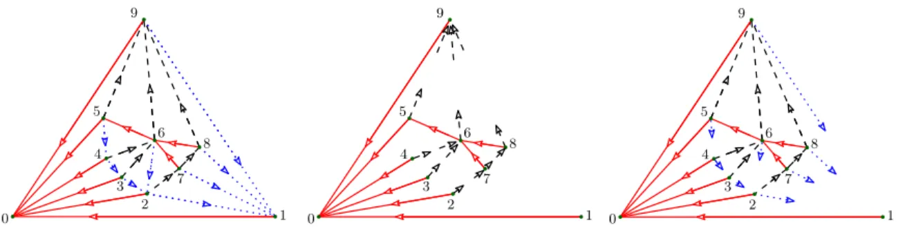
We start with a planar triangulation with n vertices, endowed with an arbitrary Schnyder wood, and we will produce a binary encoding of length 4n − 3, obtained as follows. First construct, in the classical way, a balanced parenthesis word encoding the combinatorics of the redtree: just perform a depth-first traversal of T_red starting from its root Vred and turning counterclockwise around vertices. Each time a new vertex is reached during this traversal a symbol ( is produced; while each time the traversal goes back to a parent, a symbol ) is produced. This procedure gives a word of 2n bits, called the red word in the sequel. Then we construct a black word, that stores in unary representation the number of incoming black edges (the incoming black degree of a vertex) for all vertices in G. These numbers (one for each vertex) are separated by a ’0’ symbol: vertices are naturally ordered according to the ccw-depth-first traversal of the red tree (as illustrated by the left picture in Fig. 9). Observe that the combination of the red and black words, together with the local Schnyder condition, represent the redtree enriched with the information concerning the locations of starting and ending places of black edges (depicted as broken black arrows in the middle picture of Fig.9).

The size of the final encoding can be easily evaluated, as follows. The number of 1 bits in the black word matches the number of black edges in the tree Tblack: recall that

Tblackhas n − 2 vertices and thus n − 3 edges, which leads to a total length of 2n − 3 symbols

since the black word contains a 0 bit for each vertex. The red word has two parentheses per vertex, that is a length of 2n. The total length of the encoding, concatenation of the black and redwords, is thus 4n − 3.

3 4 5 6 7 8 9 0 1 2 3 4 5 6 7 8 9 0 1 2 3 4 5 6 7 8 9 0 1 2

Figure 9: Encoding/decoding phase. A triangulation (endowed with a Schnyder wood orientation) is encoded by a pair of binary words, encoding respectively the red tree Tred and the tails of black edges (center). The information concerning blue edges is redundant and can fully retrieved by applying the local Schnyder condition (right).

is the same triangulation of the example in Figure3, where vertices are re-ordered according to the ccw-depth-first traversal of Tred):

( ( ) ( ) ( ) ( ) ( ( ( ) ( ) ) ) ( ) )00000011010101110 For the sake of clarity, we can decorate this code by vertex indices:

(0 (1 )1 (2 )2 (3 )3 (4 )4 (5 (6 (7 )7 (8 )8 )6 )5 (9 )9 )0 00 01 02 03 04 05 1106 107 108 11109.

In the example above the black word encodes the in-black-degrees of vertices, which are respectively 0, 0, 0, 0, 0, 0, 2, 1, 1, 3.

3.2 Decoding Phase

The decoding procedure is in two steps. At the first step, we use the readNextRedSymbol() to read theredword, and the operator readBlackInDegree() to retrieve the incoming black degree of vertices (stored in the black word). The linear scan of the red word allows the construction of the red tree by inserting the vertices (numbered according to the ccw-depth-traversal) into aredstack: in this way we fill allredcolumns of array C and S. In parallel, we can read the black word which allows us to fill the black columns of array C and S. No extra memory is required for an explicit storage of the red stack: as the blue columns are not involved during this first step, one bluecolumn can be used to provide an array-based implementation of such a stack.

Finally, in a second step that will be detailed later, the array of vertices is scanned retrieving the information about blueedges.

Constructing Red and Black Trees. More precisely, the red tree is entirely defined by the red word. By the coloring rule, we know that a red edge from u to v is such that LeftFront is either arededge incoming at v or a blueedge outgoing at v. Symmetrically, RightFront is either arededge incoming at v or a black edge outgoing at v. The function ConstructRedTree in Figure10(omitting the call to ConstructBlackTree) creates the

red columns of C. Observe that when the red tree is traversed in counterclockwise depth first order, the source of a black edge is always visited before its target.

We present the algorithm, in Figures 10 and 11, as recursive for the ease of com-prehension, but notice that this function does not use any implicit memory stack. We have made all memory explicit in theredand black stacks. Notice that a vertex is not simultane-ously in the two stacks (except from the top) and thus one bluearray has enough memory to implement the two stacks.

Constructing the Blue Tree When considering the red and black trees together, one obtains a planar map (an embedded graph whose faces are homeomorphic to a disk) where only blue edges are missing (as depicted in the rightmost picture of Figure 9). In the case where one is provided with a complete representation of such a map (as in [6,30]) retrieving the location of blue edges is straightforward: the source vertex of a blue edge is known by applying the local Schnyder rule (the coloring and orientation of edges around a vertex), and edge destinations can be recovered by performing a facial walk of eachred/black face. In our case such a solution cannot be applied: after the first decoding step the red and black trees are recovered, but only a partial knowledge of thered/black map is available.

Our strategy is slightly different, and consists of iteratively discovering and visiting in cw order the blue edges incident to a given vertex x (this procedure is performed in-dependently for each vertex). The code of the procedure constructBlueTree computing blue edges is illustrated by Figure 12. The code enumerates the blue edges with target x clockwise around x. Let (u, x) be a blue edge. We are searching for {v, x}, the next edge cw around x. There are four cases depending on the color of {u, v} (red or black) and of the color of {x, v} (blue or black). This can be done using Schnyder rules as described by Figure12. The three vertices Vred= 0, Vblue = 1, and Vblack= n − 1 are treated in a special

manner.

Decoding for 5n Version The above ConstructBlueTree decoding algorithm produces the 6n version of the data structure described in Section2.1. To produce the 5n version of Section2.2, the algorithm ConstructRedTree remains almost unchanged, except that S_redleft is replaced by S_redtoleft and C_redleft is replaced by C_redtoleft (taking the values red or blue instead of true or false respectively). Then, we have to modify the function ConstructBlueTree as described in ConstructBlueTree5n (Figure 13) to update the left redreferences in the relevant way, and to store only one of the two bluereferences.

3.3 Streamable Encoding Scheme

As described above, the first decoding phase (construction ofredand black trees), requires a parallel reading of the two black and red words, or to perform a linear scan of the whole encoding in two passes: to first construct the red tree, and then to recover black edges (with a second linear scan). In practice, this can be a limitation in the case of streaming applications. In order to avoid this problem, and to make our data structure fully streamable, we can slightly modify our encoding scheme, by interleaving the symbols

// N is a global counter to index vertices, initialized at 0

// before the first call, 0 is pushed in the red stack, and first ( already read. ConstructRedTree()

u = top(red stack) ; // Construct tree rooted at u d = readBlackInDegree();

ConstructBlackTree(u, d); readNextRedSymbol();

if “)” ; // u has no red child then

Ired[u] = false; else

Ired[u] = true;

N = N + 1; v = N ; // first red child of u S_redleft[v] = u; C_redleft[v] = false;

LastRedEdge=false;

while LastRedEdge == false do push(v, red stack);

ConstructRedTree() ; // tree rooted at v v=pop(red stack); u=top(red stack);

readNextRedSymbol(); if “(” then

N = N + 1; w = N ; // next red child of u S_redleft[w] = v; C_redleft[w] = true;

S_redright[v] = w; C_redright[v] = true; v = w;

else

LastRedEdge = true ; // to exit the loop end

end

// v is the last red child of u S_redright[v] = u; C_redright[v] = false; if u == 0 then

// Vred does not have outgoing black edge S_redright[v] = 1; C_redright[v] = true;

end end

if u > 1 then

// Vred and Vblue do not have outgoing black edges

push(u,black stack); end v v u u u u v w

ConstructBlackTree(u, d)

if d == 0 ; // u has no black child then

Iblack[u] = false;

else

Iblack[u] =true;

d = d − 1; pop(x,black stack) ; // first black child S_blackleft [x] = u; C_blackleft [x] = false;

while d > 0 do

y = x; d = d − 1; pop(x,black stack); S_blackleft [x] = y; C_blackleft [x] = true; S_blackright[y] = x; C_blackright[y] = true; end

S_blackright[x] = u; C_blackright[x] = false ; // last black child end x u u y u x u x d = 0 d > 0

Figure 11: This procedure performs the construction of the children of a vertex u having d incoming black edges in Tblack.

in thered and black words.

More precisely, the bits in the redand black words can be mixed in a single binary word as follows. We start with the encoding of the red tree, where ( and ) symbols are replaced by 0 and 1 bits respectively. Let us assume we are visiting and encoding a vertex v: just after the 0v bit corresponding to the first visit of v, we encode the black in-degree of

v by writing a block consisting of d 1 bits followed by a 0 bit. The mixed code corresponding to the example of Figure 9is given below

00 00 01 01 11 020212 03 03 13 040414 05 05 06 1106 07107 17 08108 18 161509 111091910. where we provide colors and subscripts just to help intuition. It is easy to distinguish betweenred and black symbols, since during the decoding phase we perform a linear scan of this mixed word, by taking into account the Schnyder local rule. We start by reading the the sequence 00001 which corresponds to the first edge (Vred, Vblue) that has no incoming

black edges. For any other vertex u (different from Vred and Vblue), when after visiting its

outgoing red edge we turn around u in ccw order, we may encounter a (possibly empty) sequence of black incoming edges.

– Thered 0u symbol must be followed by a block of black bits: a (possibly empty) sequence of black 1 bits, ended by a black 0u bit, encoding the (possibly empty) group of incoming

black edges.

– So, the black 1 symbol is always followed by a black bit.

– The red 1u symbol must be followed by a red bit. This is either a red 0v symbol (if u has another sibling vertex v in Tred) or ared 1x symbol (if x, the parent of u, has no other children).

– The black 0u symbol is followed by ared bit: either a1u bit if u has no children, or a0v bit otherwise, where v is the first child of u.

ConstructBlueTree() for x = 2 to N − 2 do

if S_redright[x] == Sleft

black[x] and C right

red [x] 6= Cblackleft [x] then

// x has no blue child Iblue[x] = false;

else

Iblue[x] = true;

if C_redright[x] ; // RightFront is red or black? then u = S_redright[x]; else z = S_redright[x]; u = S_blackright[z] ; end

// (u, x) is the first blue edge towards x S_blueright[u] = x; C_blueright[u] = false;

LastBlueEdge = false;

while LastBlueEdge==false do

// {v, x} will be the next edge cw around x;

if Ired[u] ; // (v, u) is red then

v = u + 1 ; // first red child of u if S_blackleft [x] = v and C_blackleft [x] = false then

S_blueleft[u] = x;C_blueleft[u] = false; // (u, x) last blue edge LastBlueEdge=true;

else

S_blueleft[u] = v;C_blueleft[u] = true; S_blueright[v] = u;C_blueright[v] = true; end

else

// (u, v) is black

if Sleft

black[x] 6= u then

v = S_blackright[u];

S_blueleft[u] = v;C_blueleft[u] = true; S_blueright[v] = u;C_blueright[v] = true; else

S_blueleft[u] = x;C_blueleft[u] = false; // (u, x) last blue edge LastBlueEdge=true; end end u = v; end end end or u x x u x u x v =u+1 _x or u v or u v =u+1 z u x v x

ConstructBlueTree5n() for x = 2 to N − 2 do

if Sright_red [x] == Sblackleft [x] and C right

red [x] 6= C

left

black[x] then // x has no blue child

Iblue[x] = false;

else

Iblue[x] = true;

u = Sright_red [x] ; // (u, x) is the first blue edge towards x ColorLastEdge=red; // RightFront must be red (no cw triangles) z = x;

LastBlueEdge = false;

while LastBlueEdge==false do

// {v, x} will be the next edge cw around x; if Ired[u] = true // check whether (v, u) is red

then

v = u + 1 ; // v is the first red child of u if ColorLastEdge==black then

Stoleftred [v] = z; C

toleft

red [v] =black; // Modified red ref

end

ColorLastEdge=red; if Sblackleft [x] = v and C

left

black[x] = false then

LastBlueEdge=true ; // (u, x) last blue edge Sblue[u] = x; Cblue[u] = false ; // blue ref is to the left

else

Sblue[u] = v; Cblue[u] = true;

if Ired[v] = false then

Sblue[v] = u; Cblue[v] = true;

end end else

ColorLastEdge=black ; // (u, v) is black

Sblue[u] = z ; // blue ref is to the right

if z = x then

Cblue[u] =false ; // (u, x) is first blue child

else

Cblue[u] =true;

end

if Sblackleft [x] 6= u then v = S_blackright[u];

if Ired[v] = false then

Sblue[v] = u; Cblue[v] = true;

end else

LastBlueEdge=true ; // (u, x) last blue edge end end z = u; u = v; end end end x u x u x v =u+1 x z x u u x v u v =u+1 z z ? no blue child u z = x ?

ux last blue child

ux first blue child

v

z ux last blue child

u x

v

Figure 13: Decoding algorithm: third phase for the 5n version. Changes with respect to function ConstructBlueTree are ingreen.

Thus with a simple linear scan the readNextRedSymbol and readBlackInDegree operators can be supported on the mixed encoding described above, allowing the construc-tion of thered and black trees simultaneously.

4 Experimental Results

Settings and datasets. We have written Java implementations of the processing algo-rithms and compact data structures presented in this work.4 We performed tests on a wide collection of meshes, whose sizes range from a few thousands to millions of vertices, to evaluate both the construction and navigation runtimes. Our tests involve various kinds of datasets, including several 3D models5 _{homeomorphic to a sphere as well as planar random}

triangulations generated with the uniform random sampler by Poulalhon and Schaeffer [38]. All our tests are run on an HP EliteBook, equipped with 8GB of RAM and an Intel Core i7 2.60GHz, running under linux (Ubuntu 16.04) and with Java 1.8 64-bit.

4.1 Preprocessing: construction vs. decoding.

We first evaluate the runtimes of our data structures concerning the construction phase. Table 2 shows the construction costs (expressed in seconds) of the data structure using 6n references (referred to as CDS6n, Thm 2). The runtimes reported in the first three columns correspond to the different steps in the construction phase of our data structure starting from a binary OFF file 6, which is a standard format storing both the geometry (3D vertex locations) and the mesh connectivity (the mesh is stored with a shared vertex representation). The input OFF file is read with a linear scan in order to construct on the fly, from a shared vertex representation, a half-edge data structure (using Java references) storing the triangulation in main memory (first column, building Data Structure from OFF ). The mesh is then processed in order to endow the triangulation with a Schnyder wood orientation (second column compute SW ), and finally arrays I, C and S are allocated to build the compact data structure (column building CDS6n). The overall cost of the whole pre-processing phase is given by the sum of the timing values in the first three columns. As illustrated by the runtimes reported in Table2, the timing cost is dominated by the construction of the mesh representation in main memory (see blue chart): this is the unique bottleneck of our pre-processing phase. Observe that most compact data structures [13,26–29] have the same limitation.

The runtimes of the compression algorithm are similar to the ones of the construction phase: the main difference is that it is not necessary to build our compact data structure in main memory, since the compressed file format can be obtained directly from the explicit (non compact) representation of the triangulation once it has been endowed with a Schnyder

4

A pure Java implementation of our algorithms and data structures, as well as input meshes in compressed format, are available at www.lix.polytechnique.fr/∼amturing/software.html.

5

Most of them are made available in standard format by the AIM@SHAPE Shape Repository

6

In order to obtain a fair comparison, all input data (the OFF files as well as the files storing the compressed format described in Section3.1) are stored using a binary encoding: all integer references and vertex coordinates are stored on 32 bits each.