North Indian Ocean variability during the Indian Ocean dipole

(1)

HAL Id: hal-00298501

https://hal.archives-ouvertes.fr/hal-00298501

Submitted on 9 Jun 2008

HAL is a multi-disciplinary open access

archive for the deposit and dissemination of sci-entific research documents, whether they are pub-lished or not. The documents may come from teaching and research institutions in France or abroad, or from public or private research centers.

L’archive ouverte pluridisciplinaire HAL, est destinée au dépôt et à la diffusion de documents scientifiques de niveau recherche, publiés ou non, émanant des établissements d’enseignement et de recherche français ou étrangers, des laboratoires publics ou privés.

North Indian Ocean variability during the Indian Ocean

dipole

J. Brown, C. A. Clayson, L. Kantha, T. Rojsiraphisal

To cite this version:

J. Brown, C. A. Clayson, L. Kantha, T. Rojsiraphisal. North Indian Ocean variability during the Indian Ocean dipole. Ocean Science Discussions, European Geosciences Union, 2008, 5 (2), pp.213-253. �hal-00298501�

(2)

OSD

5, 213–253, 2008

Indian Ocean variability during the

IOD J. Brown et al. Title Page Abstract Introduction Conclusions References Tables Figures ◭ ◮ ◭ ◮ Back Close Full Screen / Esc

Printer-friendly Version Interactive Discussion Ocean Sci. Discuss., 5, 213–253, 2008

www.ocean-sci-discuss.net/5/213/2008/

Ocean Science Discussions

Papers published in Ocean Science Discussions are under open-access review for the journal Ocean Science

North Indian Ocean variability during the

Indian Ocean dipole

J. Brown1, C. A. Clayson1, L. Kantha2, and T. Rojsiraphisal3

1

Geophysical Fluid Dynamics Institute, Florida State University, Tallahassee, Florida, USA

2

Department of Aerospace Engineering Sciences, University of Colorado, Boulder, Colorado, USA

3

Department of Mathematics, Burapha University, Thailand

Received: 26 March 2008 – Accepted: 8 April 2008 – Published: 9 June 2008 Correspondence to: J. Brown ([email protected])

(3)

OSD

5, 213–253, 2008

Printer-friendly Version Interactive Discussion

Abstract

The circulation in the North Indian Ocean (NIO henceforth) is highly seasonally vari-able. Periodically reversing monsoon winds (southwesterly during summer and north-easterly during winter) give rise to seasonally reversing current systems off the coast of Somalia and India. In addition to this annual monsoon cycle, the NIO circulation varies

5

semiannually because of equatorial currents reversing four times each year. These descriptions are typical, but how does the NIO circulation behave during anomalous years, during an Indian Ocean dipole (IOD) for instance? Unfortunately, in situ obser-vational data are rather sparse and reliance has to be placed on numerical models to understand this variability. In this paper, we estimate the surface current variability

10

from a 12-year hindcast of the NIO for 1993–2004 using a 1/2◦ _{resolution circulation} model that assimilates both altimetric sea surface height anomalies and sea surface temperature. Presented in this paper is an examination of surface currents in the NIO basin during the IOD. During the non-IOD period of 2000–2004, the typical equatorial circulation of the NIO reverses four times each year and transports water across the

15

basin preventing a large sea surface temperature difference between the western and eastern NIO. Conversely, IOD years are noted for strong easterly and westerly wind outbursts along the equator. The impact of these outbursts on the NIO circulation is to reverse the direction of the currents – when compared to non-IOD years – during the summer for negative IOD events (1996 and 1998) and during the fall for positive IOD

20

events (1994 and 1997). This reversal of current direction leads to large temperature differences between the western and eastern NIO.

1 Introduction

The overwhelming determinant of the circulation and its variability in the North Indian Ocean (NIO) is the seasonally reversing monsoon winds (Schott and McCreary,2001).

25

(4)

OSD

5, 213–253, 2008

Printer-friendly Version Interactive Discussion Winds south of the equator cross the equator and continue into the Arabian Sea in

the form of a strong, southwesterly low-level jet along the Somali and Oman coasts, known as the Findlater Jet. Strong upwelling occurs along these coasts and the sea surface temperature (SST) is depressed by a few degrees. During the boreal winter the winds are northeasterly and thus most major currents reverse their direction. Both the

5

southwestward flowing Somali Current north of the equator and the northward flowing East African Coastal Current south of the equator turn eastward and feed the South Equatorial Countercurrent located just south of the equator (Kantha et al.,2008). Be-tween the two monsoons, winds are westerlies along the equator and drive strong eastward-flowing surface jets along the equator known as Wyrtki-Yoshida Jets.

10

Because the winds are mostly westerlies along the equatorial waveguide, the sea surface height (SSH) is higher at the eastern side of the NIO basin. Only when the winds are anomalous and easterly does the equatorial Indian Ocean resemble the equatorial Pacific, where the prevailing winds are easterlies. The sea level is then lowered at the eastern end of the basin while upwelling takes place along the equator.

15

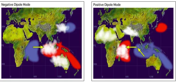
Superimposed on the “mean” circulation exists strong variability at various time scales ranging from synoptic to seasonal to interannual. The variability is moderate but can on occasion be quite large, e.g. during the Indian Ocean dipole (IOD). An IOD results when anomalously high and low SST pools occur on opposite sides of the NIO basin. This causes changes in winds, clouds, and precipitation patterns as seen in Fig. 1

20

and discussed in many previous studies (Schott and McCreary,2001;Vinaychandran et al.,2002;Webster et al.,1999, and references therein). The impact of the IOD on surface currents however is unknown because observations for the NIO have been rather sparse. No systematic monitoring system such as the TOGA-TAO array in the Pacific exists here and appeal must often be made to satellites, which monitor only the

25

conditions near the sea surface. Presented in this paper is an analysis of atmosphere and ocean parameters from a 12-year hindcast model to determine the effect of IOD events on surface currents.

(5)

OSD

5, 213–253, 2008

2 Model and data description

The numerical model used for the hindcast of the NIO is the University of Colorado version of the Princeton Ocean Model (CUPOM). This primitive equation model uses topographically conformal coordinates vertically and orthogonal curvilinear coordinates

5

horizontally. More details regarding the basic features of CUPOM can be found in Kantha and Clayson(2000).

The model used for the 12-year hindcast for the NIO study has 1/2◦_resolution hor-izontally and 38 sigma levels vertically. The simulation of the near surface circulation is improved by increasing the vertical resolution density in the first 30 levels.

Data-10

assimilation of altimetric sea surface height (SSH) anomalies and sea surface tem-perature (SST) for the CUPOM are described in great detail by Lopez and Kantha (2000a,b). Additionally, the 12-year hindcast – including numerous comparisons be-tween observations – and the hindcast results are described in detail byKantha et al. (2008).

15

3 The Indian Ocean dipole

A significant feature of the interannual oceanic and atmospheric variability in the Indian Ocean is associated with the IOD. The positive (negative) mode of this dipole, shown in the left (right) panel of Fig. 1, occurs when a cooler (warmer) than average SST pool forms in the eastern (western) Indian Ocean and a warmer (cooler) than average

20

SST pool forms in the western (eastern) Indian Ocean. Both positive and negative IOD events are marked by anomalously high surface wind stress (yellow arrows in Fig.1) and areas of increased precipitation (white patches in Fig.1). In addition to influencing the dominant air and sea patterns in the NIO, the IOD also affects the inhabitants of the region with weather extremes impacting the climate of India, Asia, Africa, and Australia, as well as the rest of the planet.

(6)

OSD

5, 213–253, 2008

Printer-friendly Version Interactive Discussion 3.1 Dipole mode index

A quantitative determination of the IOD called the dipole mode index or DMI was

de-5

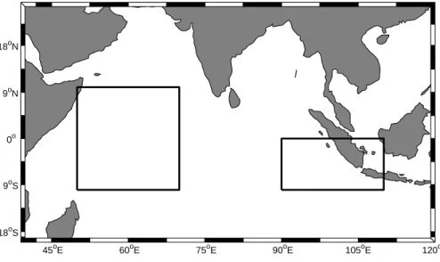
veloped byVinaychandran et al. (2002). Following the same procedure, the DMI for the 12-year hindcast is estimated as the difference between the average SST anoma-lies over the western Indian Ocean (50◦E–70◦E and 10◦S–10◦N) and the average SST anomalies over the eastern Indian Ocean (90◦E–110◦E and 10◦S–0◦), the two areas most affected by the IOD (Fig. 2). The resulting DMI in Fig. 3 is similar to that

cal-10

culated byVinaychandran et al. (2002, Fig. 2); i.e. the positive phase IOD events of 1994 and 1997, and the negative phase IOD event of 1996 are reflected in the as-similated SST hindcast data set. Negative DMI values are predominant because the normal SST difference observed across the NIO during non-IOD years is for a warmer eastern end of the basin, though most such events are not as pronounced as those of

15

1996 and 1998 when the SST difference exceeds a normalized anomaly of –2. The 1994 and 1997 positive phase IOD events both exceed a normalized anomaly value of three. There is no exacting DMI value recited in the literature that must be reached to qualify as a dipole. Instead, an IOD is qualified as such when the west-east SST difference reaches a local maximum or minimum, and the zonal SST difference across

20

the basin is reported as an indication of the strength of the dipole. Herein, 1994 and 1997 are analyzed as positive phase IOD events, while 1996 and 1998 are treated as negative phase IOD events due to each exceeding a normalized anomaly of two for a positive IOD and minus two for a negative IOD. In addition to the aforementioned IOD, there is a noticeable trend of non-IOD events for 2000-2004. Thus the NIO circulation

25

is analyzed as typical behavior (2000–2004) compared to the individual IOD years of 1994, 1996, 1997, and 1998.

3.2 IOD signature

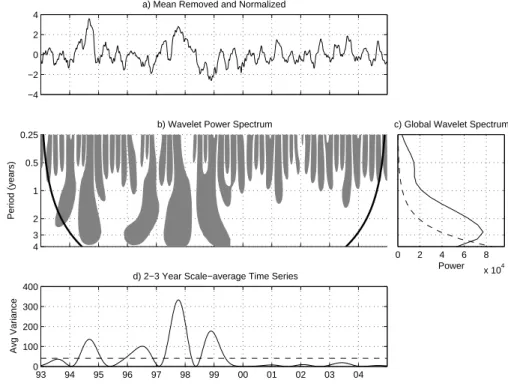
Spectral decomposition of the DMI from Fig.3 is completed using the wavelet power spectrum (WPS) developed byTorrence and Compo (1998). Throughout the 12-year

(7)

OSD

5, 213–253, 2008

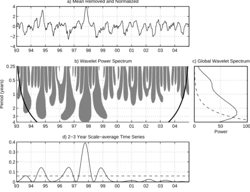
Printer-friendly Version Interactive Discussion time record, the DMI varies with a period of 0.5 years-indicated as significant contours

in Fig.4 (panel b) and the significant peak in the global wavelet spectrum (GWS) of

5

Fig.4(panel c) – which likely corresponds to the “semiannual eastward winds over the equator” (Schott and McCreary,2001). The peak in the GWS between two and three years is the result of anomalous SST differences for 19931, 1994, 1996, 1997, and 1998, as indicated by significant contours in the WPS of Fig.4(panel b). Previously, IOD events were identified for 1994, 1996, 1997, and 1998 in Fig.3. Summarily, the

10

IOD signature derived from the characteristics of the WPS in Fig. 4 is described as having 2–3 year variability superimposed on the semiannual cycle for IOD events oc-curring for 1993 to 1999, while 2000–2004 predominantly varies at the 0.5 year period and is devoid of any IOD events. Tozuka et al.(2007) similarly use a WPS to analyze the DMI resulting from a 200-year coupled general circulation model output and show

15

significant energy throughout the 1990s for both 0.5 years and between two and four years (Tozuka et al.,2007, Fig. 3).

Though the IOD is an irregular temporal occurrence, wavelet decomposition of the DMI for this particular time record delineates between years with and without IOD events when averaged for 2–3 years. For the 12-year hindcast period lasting from

20

1993 through 2004, the 2–3 year scale-average time series (SATS) in Fig.4(panel d) shows significant peaks during the IOD events of 1994, 1996, 1997, and 1998. Panel d of Fig.4is henceforth referred to as the IOD signature and is used to identify the effect of IOD events in other parameters through estimation of the 2–3 year SATS.

3.3 Empirical orthogonal function analysis of SST

Empirical orthogonal functions (EOFs) are typically used to analyze spatial and tem-poral variability in atmospheric and oceanic data. Often, however, EOF modes lack

1

The significant contour for 1993 falls inside the cone of influence and thus the results are suspicious. The cone of influence itself arises from discontinuities at the endpoints due to zero padding to reach the dyadic record length necessary for wavelet decomposition (Torrence and Compo,1998).

(8)

OSD

5, 213–253, 2008

Printer-friendly Version Interactive Discussion physical or dynamic interpretation beyond measures of statistical significance.

Fur-thermore, EOF modes are seldom the result of variability for a single period. For

5

example, a single mode may be the result of both annual and interannual variability. To reduce a dynamic event such as the IOD, which does not occur at a regular period, to a single mode is difficult. Fortunately, SST variability for 1993–2004 is replete with several highly anomalous IOD events that do occur regularly during the 1990s. When analyzed using wavelet decomposition of EOF modes for SST, IOD events are

conspic-10

uous compared to non-IOD years because of their large SST variability and regularity. In particular, the temporal variability or principal component (PC) for the 4th SST mode in Fig. 5 closely resembles that of the IOD signature in Fig. 4: significant peaks are present for 0.5 and 2–3 years in the GWS (panel c), and the 2–3 year SATS (panel d) shows significant peaks for 1994, 1996, 1997, and 1998. The WPS (Fig.5, panel b)

15

indicates that the 0.5 year period of variability is significant for all years, while the 2–3 year period of variability is exclusive to the 1990s.

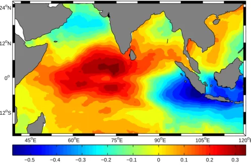
Spatial variability for the 4th SST mode, presented as a correlation map2 in Fig. 6, occurs in areas encompassed by the DMI in Fig. 1. Physical interpretation of the correlation map during the 1997–1998 IOD event, for example, follows that the blue

20

(red) contours in Fig.6are areas of anomalously low (high) SST when considering the accompanying PC in Fig. 5 (panel a). The 4th mode explains only 2%3 of the total variance of the SST field, but it is significantly different from noise according to Rule N for the record length and number of sampling locations (Overland and Preisendorfer,

2

Correlation maps are preferred for presentation of the spatial variability of EOF analysis because of understanding (Venegas et al.,1997). Each contour shows how highly correlated the area is to the temporal variability or PC. For example, dark blue contours are areas of anomolously cold SST when the PC is anomalously positive as in 1994 and 1997.

3

Though only 2% of the total variance is explained by the 4th mode, Rule N and North’s rule of thumb both suggest that the fourth mode is significant. Additionally, variability in the NIO is largely dominated by the annual cycle, which is usually associated with the monsoon. For the SST data in this study, the first three modes are dominated by the annual cycle and represent 86% of the total variance explained by the EOF decomposition.

(9)

OSD

5, 213–253, 2008

Printer-friendly Version Interactive Discussion 1982). According to North’s rule of thumb, the 4th mode is well separated from the

3rd and 5th modes when considering the 95% significance level of each (North et al.,

5

1982). Thus, the IOD signature is used to assign physical meaning to the spatial variability of the 4th SST mode by matching the temporal variability via the WPS with that of the IOD signature in Fig.4(panel d).

4 NIO dynamic response to the IOD

Section 3.3 shows the isolation of the IOD to the 4th SST EOF mode. As such, the 4th

10

mode is identified as the IOD mode because Fig.5(panel d) matches the IOD signature of Fig.4(panel d) and the overlap between areas of high correlation in Fig.6and the boxes of the DMI in Fig. 2. The isolation of the IOD signature to a single SST EOF mode is next used to identify the IOD variability in other parameters through combined EOF (cEOF). Without prior knowledge of NIO dynamics, physical interpretation of EOF

15

modes becomes difficult. Aligning variability in other parameters with that of SST via cEOF4analysis, however, estimates the simultaneous spatial and temporal variability of multiple parameters by coupling them into a single data matrix (Venegas et al.,1997; Venegas, 2001). In this study, the SST data field is paired with zonal surface wind stress (SWX), sea surface height (SSH), and zonal surface current (SCU). Analysis and the results for each pair are then referenced as: SWX, SSH, and SST-SCU. From the cEOF analysis of each pair, variability of each parameter is estimated

4

cEOF analysis is completed following the same procedure as for standard EOF analysis, with the exception of the handling of the data matrix. The parameter fields considered for analysis are normalized individually by their standard deviation, for each location, prior to being combined into a single, larger matrix. In instances where each variable is not sampled at the same locations, each measurement is further normalized by the total number of sample locations (Venegas,2001). Normalization is imperative to avoid the numerical dominance of one parameter over the other. Though sample locations are not required to coincide, each parameter must have the same temporal sampling.

(10)

OSD

5, 213–253, 2008

Printer-friendly Version Interactive Discussion as a PC for temporal variability and a correlation map for spatial variability, as with SST

in Sect. 3.3. From the cEOF analysis, the IOD signature is first identified for a particular

5

SST mode, and then variability in the corresponding mode for the coupled parameter – either SWX, SSH, or SCU – is thus associated with variability during the IOD. 4.1 SST-SWX cEOF

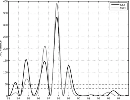
The cEOF analysis of SST and SWX estimates the 4th mode as the IOD signature from comparing the signal in Fig.4(panel d) with that of the 2–3 year SATS for SST in Fig.7

10

(black line). Both figures have significant peaks during the IOD years of 1994, 1995, 1997, and 1998. Rather than present the full WPS as in Figs.4and 5, only the 2–3 year SATS for SST is presented as an averaged summary of the WPS for comparison with the IOD signature in Fig. 4 (panel d). Variability for the 4th SWX mode is then attributed to the IOD. Temporal variability for SWX also has significant peaks for the

15

2–3 year SATS during IOD years (gray line in Fig. 7). Both time series show a peak during 1993, which, though not recognized as a negative IOD event, the DMI during 1993 shows a large negative SST anomaly across the NIO basin. Further comparison of the PCs for 4th modes of each parameter shows a correlation that is statistically significant (0.5037) at the 95% level (0.2441). The SCF explained is 0.5%.

20

The statistically significant correlation between the time series of both variables sup-ports the well established proposition that IOD events begin with an anomalous east-erly or anomalous westeast-erly wind burst near 90◦E at the equator (Schott and McCreary, 2001;Vinaychandran et al.,2002;Webster et al.,1999). This location is also found to be the area of highest correlation for the cEOF map of the 4th SWX mode in Fig.8.

Ar-25

eas of high zonal wind stress variability in Fig.8coincide with the dynamic explanation of Fig.1.

(11)

OSD

5, 213–253, 2008

Printer-friendly Version Interactive Discussion 4.2 SST-SSH cEOF

As was the case for SWX, the cEOF analysis of SST with SSH returns the 4th mode as the IOD mode in the SST parameter. Comparing the IOD signature in Fig.4(panel d) with that of the 2–3 year scale-averaged time series (SATS) of the 4th SST mode (black

5

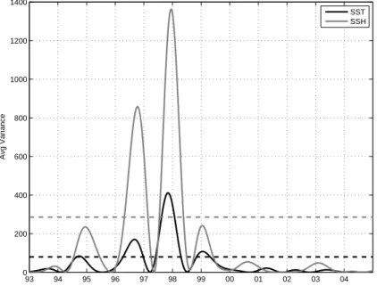
line in Fig.9) shows both signals as having significant variability during the IOD years of 1994, 1996, 1997, and 1998. The corresponding 4th SSH mode has significant peaks for 1996 and 1997, and localized peaks for 1994 and 1998 (gray line in Fig.9). The lack of significant peaks during 1994 and 1998 indicates a weaker relationship between SST and SSH variability during these years. Correlation between the PCs

10

for the 4th mode of SSH and SST (0.5934) is greater than the 95% level of 0.3020 for statistical significance (Sciremammano,1979). The square covariance fraction (SCF), analogous to the percent of total variance for the EOF analysis of a single parameter, is 2%.

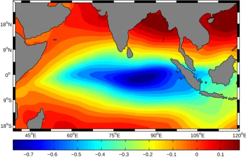
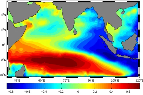
The area of highest positive correlation for spatial variability (Fig. 10) shows high

15

negative and positive correlation in areas overlapping with those of the DMI boxes in Figure 2. Spatial variability in the correlation map of Fig. 10 appears to show the existence of upwelling Kelvin waves – blue, negative contours to the east – and down-welling Rossby waves – red, positive contours to the west. The IOD is known to begin with a sharp and lasting easterly wind anomaly centered near the equator and 90◦_E

20

(yellow arrows in Fig.1). The result of such an outburst would produce Kelvin waves propagating eastward and then north and south along the coast, with complimentary Rossby waves propagating westward.Webster et al.(1999) also attributed the deepen-ing of the thermocline in the western NIO durdeepen-ing the 1997 IOD to westward-propagatdeepen-ing Rossby waves occurring south of the equator. Deepening the thermocline in the

west-25

ern NIO serves to increase the SST anomaly off the coast of Oman, thereby enhancing a positive IOD event. Though EOF analysis is not typically associated with propagating waves, persistent variability in SSH in this case is resolved as spatial variability associ-ated with the 4th mode. The pattern of the blue contours in the eastern NIO of Fig.10

(12)

OSD

5, 213–253, 2008

Printer-friendly Version Interactive Discussion suggests Kelvin waves reaching land and traveling as coastal Kelvin waves. Further,

the location of the area affected by downwelling (red contours) is consistent with the results ofWebster et al.(1999).

4.3 SST-SCU cEOF

5

Having established the cEOF analysis for SST paired with both SWX and SSH as esti-mating the temporal and spatial variability consistent with IOD dynamic explanations in the literature, the same approach is taken to estimate the zonal surface current (SCU) variability during IOD events. One of the primary interests in using the CUPOM data set is the inclusion of surface current information because of the lack of observations

10

of currents in the NIO basin. Using the model results and again working with the cEOF analysis, which identifies the portion of the NIO basin affected by the IOD, this defi-ciency can be remedied.

Consistent with the results for the IOD signature, the 2–3 year SATS for the 4th SST mode estimates the years containing an IOD event as statistically significant, i.e. the

15

black line in Fig.11has significant variability during 1994, 1996, 1997, and 1998. Thus, temporal variability in zonal surface current (SCU) of the 4th mode is attributed to the IOD. The correlation between the principal components (PCs) for the cEOF analysis of SST and SCU is 0.3026 (95% significance level is 0.2914). The SCF for the coupled 4th mode is 0.7%; modal variability for the SST-SCU pair is again dominated by the

20

annual cycle.

Spatial variability for the 4th SCU mode (Fig. 12) is along the equator extending from east to west across the NIO basin. The results for SWX – an equatorial patch of high correlation in Fig.8– complement the equatorial current variability during IOD events. Though the direction of the equatorial surface current is known to reverse

25

periodically for a given year, the results in Figs.11and12 show anomalous variability during IOD years and raises the question as to whether a change in the pattern of equatorial current reversal would produce the levels of water transport necessary to produce positive and negative dipoles.

(13)

OSD

5, 213–253, 2008

5 NIO zonal surface current variability

According to ship-drift climatology, the equatorial NIO current reverses direction three times during the year. During the monsoons in winter and summer, the equatorial

5

current flows westward. The reversal of currents eastward during spring and fall creates Wyrtki Jets with current speeds approaching 100 cm s−1. Wyrtki Jets occur during the period between the monsoons and serve to carry warmer surface water from the western NIO to the eastern side of the basin (Schott and McCreary,2001). The result of the warm water transport between the monsoons is to increase (decrease) the SST

10

and SSH in the eastern (western) NIO. 5.1 Zonal surface current during 2000–2004

The previous description of the typical current motion is observed in Fig.13 for zonal surface currents during the non-IOD years of 2000–2004. The currents are daily av-eraged near the equator (3◦S to 0◦) in the region most affected by the IOD in Fig.12.

15

Spring and fall eastward flowing currents (black contours in Fig.13) result in negative DMI values during 2000–2004 in Fig.3. In contrast, positive DMI values occur during the winter and summer for 2000–2004 in Fig.3 because of westward flowing currents represented as gray contours in Fig.13. The continuous reversal of equatorial surface currents transports water during non-IOD years to prevent the NIO from achieving a

20

west-east dipole in SST difference. As will be shown in the following sections, the IOD events observed in 1994, 1996, 1997, and 1998 are a product of changes in equatorial winds.

5.2 Zonal surface currents for the positive IOD events of 1994 and 1997

The DMI in Fig.3shows the SST difference exceeding a normalized anomaly value of

25

positive two during 1994 and 1997. Warming of the western NIO for both years follows a similar pattern: strong eastward flowing (positive) currents in the spring are followed

(14)

OSD

5, 213–253, 2008

Printer-friendly Version Interactive Discussion by an extended period of predominantly westward flowing (negative) currents for the

summer and fall. Figure15shows the evolution of the equatorial zonal surface current pattern for 1994, while the same is given for 1997 in Fig.14.

The 1997 IOD event, in particular, stands out as one of the most intense and

impor-5

tant dynamic demonstrations of air-sea interaction in the Indian Ocean basin during the hindcast time period. As a result, much of the discussion in the literature surrounding IOD events has centers on the 1997 event – sometimes referred to as the 1997–1998 event. The positive IOD of 1997 is characterized as an anomalously warm west-to-east SST difference (Webster et al.,1999, Fig. 1a) supported by an easterly wind outburst

10

(Webster et al.,1999, Fig. 1b) and the westward flowing equatorial current (Fig. 15). Both the easterly wind outburst and westward flowing equatorial, zonal surface current last until May of 1998. The positive IOD of 1994 follows the same pattern with the exception being that the westward flowing (negative) currents cease in November.

Compared to Fig.13, the equatorial current would have reversed to eastward

flow-15

ing during the winter of 1997 if not for the IOD. Instead, the current remained westward flowing into the winter where the SST warm pool was further enhanced in the west-ern NIO by the monsoon. Webster et al.(1999) credits Ekman transports and Rossby waves for deepening the western NIO thermocline, causing the SST to increase and suppressing the summer monsoon-induced coastal upwelling. If the equatorial

cur-20

rent had reversed, as is the case during non-IOD years, the warmer western water would have been transported eastward to diminish the SST difference across the basin and eliminate the IOD. The IOD instead strengthened to a normalized SST difference anomaly of four (Fig.3) and the current persisted westward through the end of the year and into the next. Ironically, the spring equatorial surface currents are strongest

east-25

ward flowing during 1997 compared to any of the 12 hindcast years. 1997 is also the strongest positive IOD which seemingly contradicts the large positive (eastward flow-ing) currents which would create a buildup of warm surface water in the eastern NIO resulting in a negative IOD.

(15)

OSD

5, 213–253, 2008

Printer-friendly Version Interactive Discussion 5.3 Zonal surface currents for the negative IOD events of 1996 and 1998

As occurred for positive and non-IOD years, the spring reversal of the equatorial cur-rents is also present for 1996 (Fig.17) and 1998 (Fig.16). For each of the 12 hindcast years the DMI in Fig.3is predominantly positive for the first half of the year. The spring

5

current reversal at the midpoint of each year causes a substantial reversal in the DMI. The obvious difference between positive and negative IOD events is the direction of the equatorial currents during the summer and fall: westward flowing (negative) currents exist for positive IOD events, while currents are eastward flowing (positive) during neg-ative IOD events. These findings are consistent with the direction of water transport

10

necessary to achieve the correct dipole difference in SST for each respective event. An interesting feature of the negative IOD events of 1996 and 1998 is the dichoto-mous equatorial current pattern of strong westward flowing (gray, negative contours in Figs.17and16) currents in the western NIO coupled with eastward flowing (black, positive contours in Figs.17and16) currents in the eastern NIO. This pattern, not

ob-15

served neither positive nor non-IOD years, occurs during August-September-October. Westward flowing currents reaching 50 cm s−1 _{in the western NIO are countered by} eastward flowing currents reaching 70 cm s−1 in the eastern half of the basin. Diver-gent equatorial surface currents near 70◦E are consistent with atmospheric divergence at the ocean’s surface and bring colder water to the surface for transportation to

oppo-20

site sides of the basin. The effect of this event on the DMI is discussed in Sect. 6. 5.4 Effect of zonal wind stress on zonal surface currents

Because equatorial surface currents are wind dominated, the behavior of the SCU is largely a result of anomalous winds. Sharp changes in the equatorial winds appear to initiate the reversal of the equatorial currents during the spring and fall. To quantify

25

this conjecture, the zonal wind stress (SWX) is averaged over the area denoted in the correlation map of Fig. 8 as being most affected by the IOD (5◦_{S to 5}◦_{N, and 70}◦_E to 95◦E). Averaging over this area produces the wind stress index, referred to here

(16)

OSD

5, 213–253, 2008

Printer-friendly Version Interactive Discussion as WSI2. Comparing WSI2 with the DMI and SCU for daily averaged values between

2000 and 2004, as in Fig.18, shows the dynamic relationship between the SST, SCU, and SWX (Fig.18). The early part of each year is marked by negative SCU and WSI2, where zonal currents induce a slight water buildup and increased SST in the western NIO until the peak during the spring. The spring and fall current reversals are shown in

5

Fig.18(black line) as sharp peaks for May and September, respectively.

The SST for the NIO basin appears to be reacting to or lagging the equatorial zonal surface currents estimated as SCU in Fig. 18 (black line). The DMI spring-peak is prevented from increasing by the sharp reversal of the zonal winds (WSI2), and con-sequently the zonal surface currents (SCU). Eastward flowing currents (positive SCU)

10

begin to transport the warmer western water across the basin during the spring – cre-ating the summer DMI peak of approximately-1 – and then reverse westward (negative SCU) for the summer and thus prevent the negative DMI peak from growing into an IOD. The dominance of westward flowing summer currents also begins the buildup of warmer water in the western NIO to create the peak in DMI observed in the fall. WSI2

15

remains positive (as westerly winds) throughout the spring and summer before de-creasing to negative for the fall and winter (as easterly winds). The currents, however, reverse direction again from westward in the summer to eastward in the fall (positive SCU) to produce a reversal in the DMI from negative to positive. Eastward flowing currents lasting throughout the fall then continue the cycle of water distribution across

20

the basin by transporting the accumulated warmer, western waters to the eastern NIO to reduce the fall DMI peak.

Wind bursts during the spring and fall (shown in Fig.18as sharp gray peaks) initiate the reversal of equatorial currents. During the summer and fall however, when equato-rial winds are positive and negative respectively, the equatoequato-rial current flows opposite

25

to the direction of the surface wind stress calculated by WSI2. As shown previously in Figs.9and10, an area of anomalous wind covering 5◦S to 5◦N and 80◦E to 95◦E is active during IOD events. The daily average for non-IOD years (black line labeled SCU in Fig. 18) is characterized by equatorial current south of the equator that flow

(17)

OSD

5, 213–253, 2008

Printer-friendly Version Interactive Discussion westward during the summer and eastward in the fall. The direction of the currents for

both periods is consistent with those with those south of the equator during the summer and winter monsoons noted bySchott and McCreary(2001). Also, zonal surface winds calculated by WSI2 are consistent with the monsoons, i.e. westerlies in the summer and easterlies in the winter.

5

In contrast to non-IOD years, IOD events are characterized by strong outbursts in equatorial winds that drive the zonal surface currents independent of the monsoon winds. Figure20compares the 1997 zonal surface currents (green line) with those of the 2000–2004 daily average (black line). The usual July decrease in the DMI occurring for non-IOD years (red line in Fig.18) is instead attenuated during 1997 by the

persis-10

tent, wind-driven summer currents (green line in Fig. 20) which are eastward flowing and serve to establish a positive dipole. The positive DMI value is then increased fur-ther when the currents, now reversed from their 2000-2004 counterparts, continue as westward flowing throughout the remainder of 1997 and into 1998. Unlike 2000–2004, the 1997 equatorial zonal currents are driven by wind stress anomalies in the area

15

covered by WSI2 instead of the monsoon winds as discussed above. This difference in wind source – equatorial surface currents driven by WSI2 winds rather than the mon-soons – is present for the summer, fall, and winter and is shown as overlapping gray and green lines for the IOD events of 1994 (Fig. 19), 1996 (Fig. 21), 1997 (Fig. 20), and 1998 (Fig.22).

20

Positive IOD events, discussed previously for FigS.14and15, are characterized by strong eastward flowing equatorial currents in the spring followed by westward flowing equatorial currents throughout the fall. Furthermore, this pattern creates a fall peak in the DMI, and a reversal in direction of the fall and winter currents compared to those of the 2000–2004 daily average. Negative IOD events differ from positive events as to the

25

seasonal peak in the DMI. A summer DMI peak for both 1996 and 1998 is attributable to the summer reversal of zonal equatorial currents from westward flowing (negative) to eastward flowing (positive). The currents are once again driven by winds in the WSI2 region. As previously noted, negative IOD events are also characterized in this study

(18)

OSD

5, 213–253, 2008

Printer-friendly Version Interactive Discussion as achieving a DMI value of minus two and persisting for the second half of the year in

question. Figure3shows the mid-2002 DMI as approaching minus two, though it is not considered here as a negative IOD event because of the brevity of this event compared

5

to those of 1996 and 1998, which both lingered into the following year.

6 Conclusions

The Indian Ocean dipole (IOD) is an important part of the air-sea dynamics of the North Indian Ocean (NIO) because of its affect on local climatology and global weather patterns. Many researchers have studied variability in various parameters during the

10

anomalous IOD years, such as sea surface temperature, sea surface height, zonal wind stress, and precipitation. Presented here are results from the analysis of the NIO circulation from surface current data – specifically zonal surface currents – produced by a 12-year hindcast using a circulation model during the period 1993–2004, which included two positive and two negative IOD events. The lack of in situ measurements

15

in the NIO and the dramatic change in local climatology during the IOD underscores the importance of these results.

Before analyzing the zonal surface current (SCU) data, the model was verified to produce the IOD events of 1994, 1996, and 1997 through estimation of the dipole mode index or DMI (Vinaychandran et al.,2002). A wavelet power spectrum (Torrence and

20

Compo,1998) was then employed to estimate an IOD signature from the DMI. The IOD signature was next used to identify the IOD mode of the EOF analysis of sea surface temperature (SST), sea surface height (SSH), and zonal wind stress (SWX). Variability for these parameters is well understood, thus providing a verification measure for the process prior to analyzing the SCU. Zonal surface current variability was then found to

25

be primarily along the equator during the IOD events of 1993–2004.

Having identified the area of variability for the SCU, the role of equatorial zonal sur-face currents during the IOD was analyzed. During the non-IOD years of 2000–2004, the equatorial SCU reverses four times each year and transports water across the

(19)

OSD

5, 213–253, 2008

Printer-friendly Version Interactive Discussion basin preventing a large SST difference between the western and eastern NIO.

Con-versely, IOD years are noted for strong easterly and westerly wind outbursts along the equator. The impact of these outbursts on the NIO circulation is to reverse the di-rection of the currents – when compared to non-IOD years – during the summer for negative IOD events (1996 and 1998) and during the fall for positive IOD events (1994

5

and 1997). Webster et al. (1999) notes the role of downwelling Rossby waves in sup-pressing the coastal upwelling due to the summer monsoon for the 1997 positive IOD mode. But the results in this study show the equatorial SCU as more than just a pas-sive observer for NIO air-sea interaction. The easterly wind burst along the equator in mid-1997 is strong and persistent enough to reverse the typical fall equatorial current

10

direction to westward. The result of the current reversal is the westward transport of warm water from the eastern NIO, which is warmed each summer by the eastward flowing, equatorial spring current. The warmer water increases the SSH and deepens the thermocline to reduce the effect of coastal upwelling from the summer monsoon. For 1997, the reversal of the current persists into the winter when the monsoon-induced

15

coastal downwelling is combined with the westward flowing current to further enhance the warming of the SST in the western NIO and extend the duration of the positive NIO. This complex interaction between the ocean surface and the atmosphere – also occur-ring duoccur-ring the IOD years of 1994, 1996, and 1998 – suggests an ENSO-like feedback involving zonal wind stress, SST, and the atmospheric pressure gradient.

20

Acknowledgements. Wavelet software was provided by C. Torrence and G. Compo, and is

available at URL:http://paos.colorado.edu/research/wavelets/.

References

Kantha, L. H. and Clayson, C. A.: Numerical Models of Oceans and Oceanic Processes, 940 pp., Academic Press, San Diego, California, USA, 2000.

25

(20)

OSD

5, 213–253, 2008

variability as seen in a numerical hindcast of the years 1993 to 2004, Progress in Oceanog-raphy, 76, 111–147, 2008.

Lopez, J. W. and Kantha, L. H.: Results from a numerical model of the northern Indian Ocean: circulation in the South Arabian Sea, J. Mar. Syst., 24, 97–117, 2000a.

Lopez, J. W. and Kantha, L. H.: A data-assimilative model of the north Indian Ocean, J. Atmos. Oceanic Technol., 17, 1525–1540, 2000b.

North, G. R., Bell, T. L., Cahalan, R. F., and Moeng, F. J.: Sampling error in the estimation of 5

empirical orthogonal functions, Mon. Wea. Rev., 110, 699–706, 1982.

Overland, J. E. and Preisendorfer, R. W.: A significance test for principal components applied to a cyclone climatology, Mon. Wea. Rev., 110, 1–4, 1982.

Schott, F. A. and McCreary, J. P.: The monsoon circulation of the Indian Ocean, Progress in Oceanography, 51, 1–123, 2001.

10

Sciremammano, F.: A suggestion and resentation of correlations and their significance levels, J. Phys. Oceanogr., 9, 1273–1276, 1979.

Torrence, C. and Compo, G. P.: A practical guide to wavelet analysis, Bull. Amer. Meteor. Soc., 79, 61–78, 1998.

Tozuka, T., Luo, J., Masson, S., and Yamagata, T.: Decadal modulations of the Indian Ocean 15

dipole in the SINTEX-F1 coupled GCM, J. Climate, 20, 2881–2894, 2007.

Venegas, S. A.: Statistical methods for signal detection in climate, Danish Center for Earth 460

System Science (DCESS) Report #2, 96 pp., Niels Bohr Institute for Astronomy, Physics and Geophysics, University of Cophenhagen, Denmark, 2001.

Venegas, S. A., Mysak, L. A., and Straub, D. N.: Atmosphere-ocean coupled variability in the South Atlantic, J. Climate, 10, 2904–2920, 1997.

Vinaychandran, P. N., Iizuka, S., and Yamagata, T.: Indian Ocean dipole mode events in an 465

ocean general circulation model, Deep-Sea Res. Part II, 49, 1573–1596, 2002.

Webster, P. J., Moore, A. M., Loschnigg, J. P., and Leben, R. R.: Coupled ocean-atmosphere dynamics in the Indian Ocean during 1997-98, Nature, 401, 356–360, 1999.

(21)

OSD

5, 213–253, 2008

Fig. 1. Air-sea interaction for a negative (left panel) and a positive (right panel) IOD event.

Red (blue) contours indicate anomalously warm (cold) SST values. The dominant wind stress pattern is indicated by the yellow arrows. Areas of anomalously high precipitation are shown as white patches. Source:http://www.jamstec.go.jp/frsgc/research/d1/iod/.

(22)

OSD

5, 213–253, 2008

Printer-friendly Version Interactive Discussion 45oE 60oE 75oE 90oE 105oE 120oE 18oS 9oS 0o 9oN 18oN

(23)

OSD

5, 213–253, 2008

Printer-friendly Version Interactive Discussion 93 94 95 96 97 98 99 00 01 02 03 04 −2 −1 0 1 2 3 Normalized Anomaly

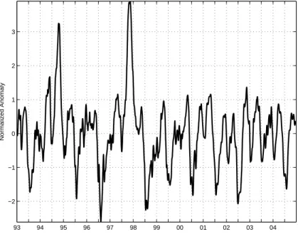
Fig. 3. Calculated DMI from the anomaly in SST when subtracting the area average for the

west and east boxes in Fig.2. The time series has the mean removed and is normalized by its standard deviation. IOD events for 1994, 1996, 1997, and 1998 appear as SST anomalies (Vinaychandran et al.,2002).

(24)

OSD

5, 213–253, 2008

Printer-friendly Version Interactive Discussion 93 94 95 96 97 98 99 00 01 02 03 04 −4 −2 0 2 4

a) Mean Removed and Normalized

93 94 95 96 97 98 99 00 01 02 03 04 0.25 0.5 1 2 3 4 Period (years)

b) Wavelet Power Spectrum

0 50 100 Power c) Global Wavelet Spectrum

93 94 95 96 97 98 99 00 01 02 03 04 0 0.1 0.2 0.3 0.4

d) 2−3 Year Scale−average Time Series

Fig. 4. Wavelet analysis of the DMI in Fig.3. Panel (a) is the DMI, panel (b) is the wavelet power spectrum (WPS), panel (c) is the global wavelet spectrum (GWS), and panel (d) is the 2–3 year scale-average time series (SATS). The 95% significance level – gray contours in panel b and the dashed lines in panel c and panel d – are estimated using a lag-1 red noise background spectrum. The thick lines in panel b are the boundaries for the “cone of influence” and indicate areas of the WPS affected by edge effects. A two-parameter DOG wavelet was used in the analysis. Panel c, the GWS, is estimated by averaging across the time record (horizontally) at each period. Panel d, the SATS, is estimated by averaging vertically across the two-three year period for each day of the time record.

(25)

OSD

5, 213–253, 2008

Printer-friendly Version Interactive Discussion −4 −2 0 2 4

a) Mean Removed and Normalized

0.25 0.5 1 2 3 4 Period (years)

b) Wavelet Power Spectrum

0 2 4 6 8 x 104 Power c) Global Wavelet Spectrum

93 94 95 96 97 98 99 00 01 02 03 04 0 100 200 300 400 Avg Variance

d) 2−3 Year Scale−average Time Series

Fig. 5. Wavelet analysis of the principal component of the 4th SST mode, which explains

2% of the total variance. Each of the panel descriptions and the wavelet parameters used for significance are the same as for Fig.4.

(26)

OSD

5, 213–253, 2008

Printer-friendly Version Interactive Discussion 45oE 60oE 75oE 90oE 105oE 120oE 12oS 0o 12oN 24oN −0.5 −0.4 −0.3 −0.2 −0.1 0 0.1 0.2 0.3

Fig. 6. EOF correlation map for the 4th SST mode. Correlation contours greater than ±0.130,

(27)

OSD

5, 213–253, 2008

Printer-friendly Version Interactive Discussion 93 94 95 96 97 98 99 00 01 02 03 04 0 50 100 150 200 250 300 350 400 Avg Variance

2−3 Year Scale−Average Time Series

SST SWX

Fig. 7. Two to three year SATS for SST (black line) and SWX (gray line) for the fourth mode

of each resulting from the cEOF analysis. The dashed lines and wavelet parameters used to calculate the WPS from which the SATS of each variable are the same as those used in Fig.4.

(28)

OSD

5, 213–253, 2008

Printer-friendly Version Interactive Discussion 45oE 60oE 75oE 90oE 105oE 120oE 18oS 9oS 0o 9oN 18oN −0.7 −0.6 −0.5 −0.4 −0.3 −0.2 −0.1 0 0.1

Fig. 8. Correlation map of the 4th SWX mode from cEOF analysis with SST. The area of

anomalously high SWX in the eastern Indian Ocean occurs along the equator (as in Fig.1), with contours greater than ±0.128 (in absolute value) being statistically significant at the 95% level.

(29)

OSD

5, 213–253, 2008

Printer-friendly Version Interactive Discussion 93 94 95 96 97 98 99 00 01 02 03 04 0 200 400 600 800 1000 1200 1400 Avg Variance

2−3 Year Scale−Average Time Series

SST SSH

Fig. 9. Two to three year SATS for SST (black line) and SSH (gray line) for the fourth mode

(30)

OSD

5, 213–253, 2008

Printer-friendly Version Interactive Discussion 45oE 60oE 75oE 90oE 105oE 120oE 18oS 9oS 0o 9oN 18oN −0.8 −0.6 −0.4 −0.2 0 0.2 0.4 0.6

Fig. 10. Spatial variability for the 4th SSH mode from cEOF analysis with SST. Contours greater

(31)

OSD

5, 213–253, 2008

Printer-friendly Version Interactive Discussion 93 94 95 96 97 98 99 00 01 02 03 04 0 50 100 150 200 250 300 350 400 Avg Variance SST SCU

Fig. 11. Two to three year SATS for SST (black line) and SCU (gray line) for the fourth mode

(32)

OSD

5, 213–253, 2008

Printer-friendly Version Interactive Discussion 45oE 60oE 75oE 90oE 105oE 120oE 18oS 9oS 0o 9oN 18oN −0.7 −0.6 −0.5 −0.4 −0.3 −0.2 −0.1 0 0.1 0.2 0.3

Fig. 12. Spatial variability for the 4th SCU mode from cEOF analysis with SST. Contours greater

(33)

OSD

5, 213–253, 2008

Printer-friendly Version Interactive Discussion −30 −30 −30 −30 −30 −30 −30 −30 −10 −10 −10 −10 −10 −10 −10 −10 −10 −10 −10 −10 −10 −10 −10 −10 −10 −10 −10 −10 −10 −10 −10 −10 10 10 10 10 10 10 10 10 10 10 10 10 10 10 10 10 10 10 10 10 10 10 10 10 10 10 10 10 10 10 10 10 10 ₁₀ 10 10 10 10 10 30 30 30 30 30 30 30 30 30 30 30 30 30 30 30 50 50 50 50 50 50 70 70

40E 50E 60E 70E 80E 90E 100E

Jan Feb Mar Apr May Jun Jul Aug Sep Oct Nov Dec

Fig. 13. 2000–2004 daily averaged zonal surface current (SCU) evolution in cm s−1. Values are averaged between 3◦_{S and 0}◦_{. The range of positive SCU (black contours) is 10 to 70 cm s}−1_.

Negative SCU (gray contours) values extend from –30 to –10 cm s−1_{. Both positive and negative}

(34)

OSD

5, 213–253, 2008

Printer-friendly Version Interactive Discussion −70 −50 −50 −50 −50 −50 −50 −30 −30 −30 −30 −30 −30 −30 −30 −30 −30 −30 −30 −30 −30 −30 −30 −30 −30 −30 −30 −30 −30 −30 −30 −30 −30 −30 −30 −30 −30 −30 30 30 30 30 30 30 30 30 30 30 30 30 30 30 30 30 30 30 30 30 30 30 30 30 30 30 30 30 30 30 30 30 30 30 30 30 30 30 50 50 50 50 50 50 50 50 50 50 50 50 50 50 50 50 50 50 50 50 70 70 70 70

40E 50E 60E 70E 80E 90E 100E

Fig. 14. SCU evolution in cm s−1_{during the positive IOD of 1994. Values are averaged between}

3◦S and 0◦. The range of positive SCU (black contours) is 30 to 70 cm s−1. Negative SCU (gray contours) values extend from –70 to –30 cm s−1_{. Both positive and negative contours are}

(35)

OSD

5, 213–253, 2008

Printer-friendly Version Interactive Discussion −90 −70 −70 ₋₇₀ −70−70 −70 −70 −70 −70 −70 −70 −70 −70 −50 −50 −50 −50 −50 −50 −50 −50 −50 −50 −50 −50 −50 −50 −50 −50 −50 −50 −50 −50 −50 −50 ₋₅₀ −30 −30 −30 −30 −30 −30 −30 −30 −30 −30 −30 −30 −30 −30 −30 −3 0 −30 −30 −30 −30 −30 −30 −30 −30 −30 −30 −30 −30 −30 −30 −30 −30 −30 −30 −30 −30 −30 −30 −30 −30 −30 −30 −30 −30 −30 −30 −30 −30 −30−30 ₋₃₀ −30 −30 −30 −30 30 30 30 30 30 30 30 30 30 30 30 30 30 30 30 30 3030 30 30 30 50 50 50 50 50 50 50 70 70 90 110 110

40E 50E 60E 70E 80E 90E 100E

Fig. 15. SCU evolution in cm s−1during the positive IOD of 1997. Values are averaged between 3◦_{S and 0}◦_{. The range of positive SCU (black contours) is 30 to 110 cm s}−1_{. Negative SCU}

(gray contours) values extend from –70 to –30 cm s−1_{. Both positive and negative contours are}

(36)

OSD

5, 213–253, 2008

Printer-friendly Version Interactive Discussion −50 −50 −50 −50 −50 −50 −50 −50 −50 −50 −50 −50 −50 −50−50 −50 −30 −30 −30 −30 −30 −30 −30 −30 −30 −30 −30 −30 −30 −30 −30 −30 −30 −30 −30 −30 −30 −30 −30 −30 −30 −30 −30 −30 −30 30 30 30 30 30 30 30 30 30 30 30 30 30 30 30 30 30 30 30 30 30 30 30 30 30 30 30 30 30 30 30 30 30 30 30 30 30 30 30 30 30 30 30 30 30 30 30 30 30 50 50 50 50 50 50 50 50 50 50 50 50 50 50 50 50 50 50 50 50 50 50 50 50 50 50 50 50 50 50 50 50 50 50 70 70 70 70 70 70 70 70 70 70 70 70 70 70 70 70 70 90 90 90 90 90 110

40E 50E 60E 70E 80E 90E 100E

Fig. 16. SCU evolution in cm s−1 during the negative IOD of 1996. Values are averaged between 3◦_{S and 0}◦_{. The range of positive SCU (black contours) is 30 to 110 cm s}−1_{. Negative}

SCU (gray contours) values extend from –50 to –30 cm s−1_{. Both positive and negative contours}

(37)

OSD

5, 213–253, 2008

Printer-friendly Version Interactive Discussion −50 −50 −50 −50 −50 −50 −50−50 −30 −30 −30 −30 −30 −30 −30 −30 −30 −30 −30 −30 −30 −30 −30 −30 −30 −30 −30 −30 −30 −30 −30 −30 −30 −30 −30 −30 −30 −30 −30 30 30 30 30 30 30 30 30 30 30 30 30 30 30 30 30 30 30 30 30 30 30 30 30 30 30 30 30 30 50 50 50 50 50 50 50 50 50 50 50 50 50 50 50 50 50 50 50 50 50 70 70 70 70 70 70 70 70 70 70 90 90 90 110

40E 50E 60E 70E 80E 90E 100E

Fig. 17. SCU evolution in cm s−1 _{during the negative IOD of 1998. Values are averaged}

between 3◦S and 0◦. The range of positive SCU (black contours) is 30 to cm s−1. Both positive and negative contours are presented in increments of 20 cm s−1_.

(38)

OSD

5, 213–253, 2008

Jan Feb Mar Apr May Jun Jul Aug Sep Oct Nov Dec −4 −3 −2 −1 0 1 2 3 4 5 SCU DMI WSI2

Fig. 18. Comparison of the SCU (averaged over 3◦_{S to 0}◦_{and 70}◦_{E to 95}◦_{E), the dipole mode}

index (DMI), and the zonal wind stress index (WSI2, averaged over 5◦_{S to 5}◦_{N and 80}◦_{E to}

95◦_{E) during the non-IOD years of 2000–2004. The SCU (black line) and the WSI2 (gray line)}

are daily averaged for 2000–2004, and then the area average is estimated. The DMI is daily averaged from the values in Fig.3for the 2000–2004 period. Each time series has the mean removed and is normalized by its respective standard deviation for comparison.

(39)

OSD

5, 213–253, 2008

Jan Feb Mar Apr May Jun Jul Aug Sep Oct Nov Dec −4 −3 −2 −1 0 1 2 3 4 5 1994 2000−2004 DMI WSI2

Fig. 19. Comparison of the SCU (averaged over 3◦_{S to 0}◦ _{and 70}◦_{E to 95}◦_{E) for 1994 (green}

line) and 2000–2004 (black line), the dipole mode index (DMI) for 1994, and the zonal wind stress index (WSI2, averaged over 5◦_{S to 5}◦_{N and 80}◦_{E to 95}◦_{E) during 1994. The SCU}

(black line) is daily averaged for 2000–2004, and then the area average is estimated. The DMI is daily averaged from the values in Fig.3for the 2000–2004 period. Each time series has the mean removed and is normalized by its respective standard deviation for comparison.

(40)