Design of human-like posture prediction for inverse kinematic posture control of a humanoid robot

(1)

Design of Human-Like Posture Prediction for Inverse Kinematic posture

control of a Humanoid Robot

by

Derik Thomann

Submitted to the Department of Mechanical Engineering

in partial fulfillment of the requirements for the degree of

Bachelor of Science in Mechanical Engineering

at the

rm

acnd

MASSACHUSETTS INSTITUTE OF TECHNOLOGY

© Derik Thomann, MMV. All rights reserved.

The author hereby grants to MIT permission to reproduce and

distribute publicly paper and electronic copies of this thesis document

in whole or in nart

~~~~~~~Author· .

A

.

Author7 ;~./..<. · ~ ~ ' . .£

Department of Mechanical Engineering

May 6, 2005

Certified

)

by

. ... ...

..

.. .... ...

Cynthia Breazeal

Assistant Professor

Thesis Supervisor

Accepted

by

.

...

Ernest Cravalho

Chairman, Undergraduate Thesis Committee

(2)

(3)

Design of Human-Like Posture Prediction for Inverse Kinematic posture control of a Humanoid Robot

by

Derik Thomann

Submitted to the Department of Mechanical Engineering

on May 6. 2005 in partial fulfillment of the

requirements for the degree of

Bachelor of Science in Mechanical Engineering

Abstract:

A method and system has been developed to solve the kinematic redundancy for a

humanoid redundant manipulator based on forward kinematic equation and the optimization of human-like constraints. The Multiple Objective Optimization (MOO) is preformed using

a Genetic Algorithms (GA) and implemented using the Genetic and Evolutionary

Algorithm Matlab Toolbox. The designed system is illustrated on a simple redundant 3 degree of freedom (dof) manipulator and is set up for a more complicated redundant 7 dof

manipulator. The 7 dof manipulator is modeled from the Stan Winston studio's Leonardo, an 61 dof expressive humanoid robot. It has been found that the inverse kinematic solution to a 3dof model arm converged within 1% error of the solution within .05 mins processor time using the discomfort human-like constraint in 2d space. Similarly, the inverse kinematic solution to a 7 dof model arm consisting of Leonardo's right arm geometry was found to converge within 1% error within .20 mins processor time using the discomfort human-like constraint in 3D space. The full kinematic model of Leonardo is developed and future efficiency optimizations are posed to move towards the real-time motion control of a

redundant humanoid robot by way of human-like posture prediction.

Thesis Supervisor: Cynthia Breazeal Title: Assistant Professor

(4)

(5)

Acknowledgments

The completion of this document would not be possible without the help and guidance of many: Special thanks to Professor Cynthia Breazeal, for supervision of my thesis work and everything else she has helped me with during my time at MIT.

Thanks to the members of the Robotic Life Group for giving me a temporary home in a extremely creative environment. I hope in the end the research I performed is useful to them.

Thanks to Professor Haruhiko Asada for teaching the experimental class Introduction to Robotics and sparking my interest in robotics.

Thanks to Professor Dan Frey for his guidance and encouragement to constantly explore and apply cross-disciplinary knowledge to find new solutions.

And of course thanks to my family and friends: To my Mom for letting me take apart everything, including the tv (I still haven't gotten it back together right), and to my Dad for always giving me

an engineering role model to aspire to be more like. To the ol' 2.007x gang, FeCl2, and the best

learning environment ever. Most of all to Amy for always being there and keeping me relativity sane and happy with the world.

(6)

(7)

List of Figures

Figure 1-1 An image of three dots, used for the illustration of a humanoid manipulator's (human arm's) redundancy. By placing two of your fingers and your thumb in one of each of these 3 dots, you essentially constrain the end effector (finger) position solution of your arm. The rotation of your arm after your fingers have been constrained illustrates the infinite dimension of the joint space solutions for this position. This defines the task of which arm posture to choose, a common problem in humanoid robotics ...

Figure 2-1 Two joint primitives of the revolve joint and the prismatic joint, commonly used to form ideal models of robots for kinematic analysis ...

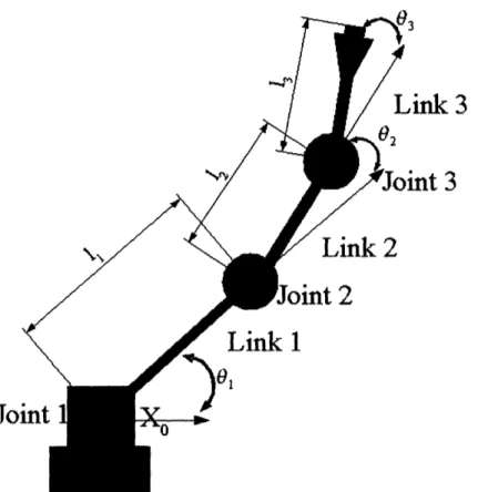
Figure 2-2 A three link robotic manipulator, made of three revolve joints with joint

variables 01, 02, and03 ...

Figure 2-3 Two links of a larger robotic system, illustrating the definition of axis

necessary for Denavit-Hartenberg Representation. ...

Figure 2-4 Figure 3-1 15 19 20 21 24

Two redundant serial planar robots possessing the same end effector solution but having different joint solutions, or different postures ...

Graphical output of the first 30 generation of a Multiple Objective Optimization problem. The upper left graph shows the convergence of the range of values towards the objective value of 0. The second graph from the upper left shows the convergence towards a optimal solution in the best individual from each generation. Out of the chaos at the beginning, an order seems to emerge and you can try to interpret the results. The upper rightmost

(10)

bottom leftmost graph shows the value of each variable in all members of the current generation, this two distinct shapes in this graph show two possible optimal solutions. The bottom middle graph shows the objective values of the individuals of the current generation while the bottom right graph shows

the order of the subpopulations ... 29

Figure 4-1 A photo of Leonardo, the emotionally expressive humanoid robot. Copyright

Sam Ogden. Leonardo character design copyright Stan Winston Studio ... 34

Figure 6-1 SolidWorks solid model of Leonardo, modeled from the original part

drawings provided by Stan Winston Studio ... 36

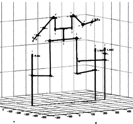
Figure 6-2 Matlab Robotics Toolbox representation of Leonardo, up to the head. This model is constructed from 3 mutually distinct serial chains. This form of Leonardo is very useful for kinematic calculations. The D-H representation

of this model appears in appendix ... 37

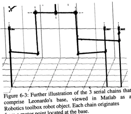
Figure 6-3 Further illustration of the 3 serial chains that comprise Leonardo's base, viewed in Matlab as a Robotics toolbox robot object. Each chain originates

from a motor point located at the base ... 38

Figure 6-4 A plot of Leonardo's torso and right arm subsystem from Jeff Lieberman's

Robotics Toolbox model ... 39

Figure 6-5 A plot of Leonardo's right arm subsystem to contrast aspects of the new

design, viewed in Matlab as a Robotics toolbox robot object ... 40

(11)

posture prediction, viewed in Matlab as a Robotics toolbox robot object. This arm is equivalent to a humanoid arm held up at shoulder level and constrained to horizontal in plane movements ...

Figure 8-2 An in plane plot of the final solution of 3dof planar example, viewed in Matlab as a Robotics toolbox robot object. Final orientation solved for with desired position solution space further constrained by the discomfort

metric...

Figure 8-3 A plot of the other possible end effector solution, viewed in Matlab as a

Robotics toolbox robot object. Solved for by imposing a maximum

discomfort

...

Figure 8-4 A screen shot of a single unconstrained(without discomfort objective) GA

after 30 generations, notice the divergence from the objective in the graph on the top left. The upper middle plot shows the "confusion" between solutions in the best individual from each generation, In fact none of these generations come close to producing an individual with the correct end-effector solution. The bottom leftmost graph shows the value of each variable in all members of the current generation, this "looped" box shape shows the competition between two optimal solutions...

Figure 8-5 A screen shot of the MOO after 60 generations, but notice an almost immediate convergence towards an optimal solution. The upper left graph shows the extreme minimization of the objective value. The second graph from the upper left shows the optimal solution in the best individual from each generation. This is a striking graphic as it shows how close a member of each generation is to the optimal solution. The bottom leftmost graph shows the value of each variable in all members of the current generation, this single distinct shape shows a well constrained optimal solutions...

44

47

48

(12)

(13)

List of Tables

Table 1 The Physical Interpretation of D-H Parameters ... 23

(14)

(15)

Chapter 1 Introduction

1.1 Why Posture Control

Set this thesis down and place two fingers on the colored circles below in Figure [1-1]. Now place your thumb on the white circle. Without losing contact with the page try and move your arm around. Now, try to experiment with putting your arm in your lap and reconnecting with the circles; notice how your arm settles into approximately the same orientation each time.

Figure 1-1: An image of three dots, used for the illustration of a humanoid manipulator's (human arm's) redundancy. By placing two of your fingers and your thumb in one of each of these 3 dots, you essentially constrain the end effector (finger) position solution of your arm. The rotation of your arm after your fingers have been constrained illustrates the infinite dimension of the joint space solutions for this position. This defines the task of which arm posture to choose, a common problem in humanoid robotics.

(16)

What was just shown is a result recognized in ergonomic design [6][12], and in anamorphic simulations[18]. Even when multiple joint configurations or postures are possible, a human is most likely to choose the posture that minimizes some metric of discomfort. This principal has been used in ergonomic design to produce minimum stress workspaces [12]. Rather then use this idea for workspace and task design, I will take inspiration from ergonomics and neuroscience to design a method for the control of an humanoid robot arm.

Posture is very important in humanoid robotics. The reaching movements with similar hand paths but different arm orientations are qualitatively dissimilar. The posture of the arm affects the kinematics, and not only by spatial attributes of the hand trajectory. In order to control the motion of a humanoid robot, we must be able to distinguish human-like postures for other feasible solutions.

1.2 A Possible Application in Learning by Demonstration

When a task requires the dexterity or manipulability of humans, learning by demonstration has been used to show a robot how it must perform a task. Jeff Lieberman and Cynthia Breazeal designed a system that produced a generalized trajectory from relatively few action trails [1]. A human actor performs an action in a Teleoperation suit, which is recorded. The suit records the absolute movements which then are geometrically transformed to determine the actual extem joint angles acted out by the robot actor. Movement data is next analyzed through a stereo optic camera. Tactile data is recorded throughout each trial. Motion segmentation is performed by creating start and end markers for each episode based on Mean Squared Velocity (MSV). Similar episodes are combined and further manipulation produces final episode boundary

(17)

selection. The trails are analyzed to create two Radial Basis Functions (RBF) solutions, one to preserve the quality of motion, and one to retain end effector precision. These two solutions are then blended to achieve extremely complicated interactions.

The implement of this algorithm used the inverse Jacobian method (ie. Dq = J- dx), also called the resolved motion method, to move the end effector to the desired position from an initially defined position [2]. In general, this method suffers two major weak points; the method has inaccuracy due to linear approximation, and also does not give a direct joint variable solution for a desired end-effect position [3]. In a redundant chain manipulator, this solution suffers another major problem which will be identified in the chapter on inverse kinematics.

Since only the end-effector is fully defined by the learning by demonstration algorithm, feasible joint angles still need to be determined. The problem presented is; given a reachable position in the work space, what is a realistic posture.

(18)

(19)

Chapter 2 Robot Kinematics

2.1 Basics of Robot Kinematics

A robot mechanism is a multi-body system made of rigid bodies called links. Connection between the links are made by two types of joints, shown in Figure [1-2]. The revolve joint is where a pair of link rotate around the same fixed axis. The prismatic joint, also called the sliding joint, is where two links make translational displacements along a fixed axis. Basic forward kinematics calculates the position of the end-effector in absolute coordinates based on the fully

I

Revolve Joint

Prismatic Joint

Figure 2-1: Two joint primitives of the revolve joint and the prismatic joint, commonly used to form ideal models of robots for kinematic analysis.

defined joint positions. Consider the 3 degree of freedom arm shown in Figure [1-3]. The arm is made of one fixed link and 3 mobile links with parallel axis so all movement occurs within the

plane. In order to completely define the joint positions, the link lengths [ l, 12, 13] must be known,

(20)

relation between the end effector coordinates and the joint angles is given by equation

0.

Xe I1 Co(01) +12 cos (0 +02)+13 COS (01 +02+03)

Ye=ll

sin (0

1

)+l

2

sin (0

1

+0

2

)+1

3

sin

(01+02+03)

3

3 Link 1 PI f 1 4' 0Z _

Jo

Figure 2-2: A three link robotic manipulator, made of three revolve joints with joint variables

E , 2 , and [13

2.2 Denavit-Hartenberg Convention

Unfortunately, forward kinematics does not stay so simple. The kinematics of serial chains of manipulators becomes increasingly difficult with the number of links added. The Denavit-Hartenberg convention (Denavit-Denavit-Hartenberg 1955) is used to aid the simple construction of the

(21)

kinematics of series manipulator chains. Also the D-H convention allows the construction of the forward kinematic relation by the multiplication of homogeneous joint coordinate transform matrices.

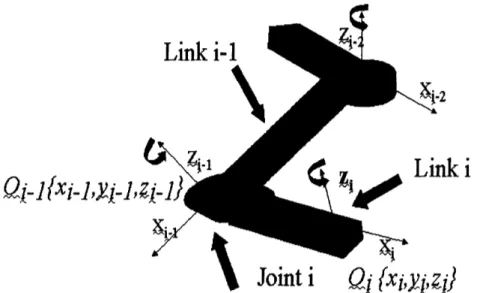
As seen in Figure [2-3], a robot comprised of n joints has n+l links. Joint i connects link

i-I to link i. We consider joint i to be fixed with respect to link i-i (ie. When Joint i is moved,

link i rotates about its center of rotation). To construct a D-H representation, we rigidly attach a coordinate frame to each link. Any set of coordinate frame will work as long as the axis xi is perpendicular to zi, and axis x intersects z.

i-2

Link i

1%

Joint i

0i

(xiY,

]

Figure 2-3: Two links of a larger robotic system, illustrating the definition of axis necessary for Denavit-Hartenberg Representation.

We can express Ojxjyj,zj with respect to Oi[xiyiz] using the homogeneous joint configuration

dependent transform A.. iRj(q) is the rotation matrix and X (q) is the position vector.

I.;

(22)

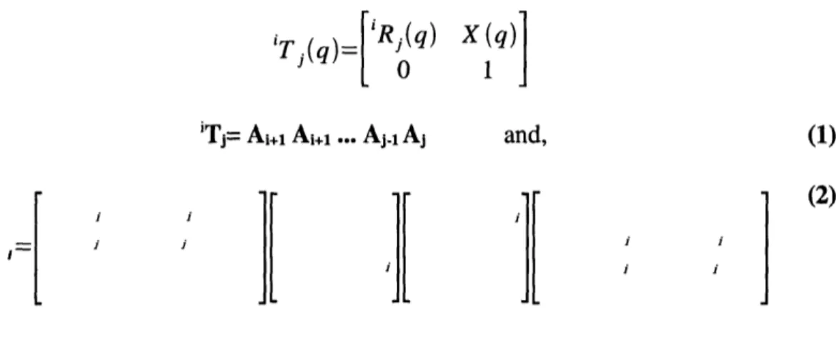
i'T ~ ) ARj( q) X (q)

Tj(q)= 0

iTj= Am~ Aim ... Aj-1iAj and,

i]l

(1) (2)

il]

Note that Tj' is the homogeneous transformation matrix relating i to j, and is configuration dependent through the set of four D-H parameters in equation 2. The values [ai,o i,di ,Oi] form the complete representation of the homogeneous transform for link i. Table [1] translates the D-H parameters into physical interpretations.

Table 1: The Physical Interpretation of D-H Parameters

In standard revolve joints, only the value of Oi is variable. This leads to the convention of

ai distance between zi-I and zi

(i angle between zi- and zi measured in plane normal to xi

di distance between Oi-, and the intersection of the xi axis with

zi-measured along the zi-I axis

(23)

zi-referring to Oi as the joint variable. Similarly for prismatic joints, only is di is defined as the

joint variable.

2.3 Inverse Kinematics

Inverse kinematics computes the joint variable solutions that correspond to a particular end effector position. This provides an easy way to manipulate every joint in a kinematic chain: a desired posture can be define by only defining a few points and allowing an algorithm to determine the rest of the joint configuration. The inverse kinematic (K) equation is the inverse

of the kinematic equation (0). Given the end effector position (Oe{xe,ye.ze}) and the inverse

kinematic transform (A) the joint angles (q) required are simply given in equation (2.3.1).

q =A Oe{xe,Ye.Ze} (2.3.1)

Robotic arms are defined as kinematically redundant when the number of joints is greater than the number of degrees of freedom needed to describe a task in the task space. Redundancy in 2D space is shown in Figure [1-5]. In the field of robotics in general, the task requirement is for an end effector to reach a position at a particular orientation in three dimensional (Cartesian) space. The general form of this movement requires 6 degrees of freedom, and therefore any robot with more than 6 independent joints is a redundant robot. In a redundant system when the end effector is in a fixed position, some number of joints are still free to move. Each redundancy/redundant joint creates an extra independent variable for the system. Therefore, due to redundant degrees of

(24)

ZIL~

-4

Figure 2-4: Two redundant serial planar robots possessing the same end effector solution but having different joint solutions, or different postures.

freedom in a humanoid arm, a family of solutions rather than a unique solution is produced when

(25)

an end effector position and orientation is specified. Redundant IK solutions can be differentiated based on their distinct posture, and can be useful for optimizing a cost function, keeping away from joint limits, and avoiding collisions and Jacobian singularities.

2.4 Inverse Kinematic Methods

At the highest level, inverse kinematic methods can be describe as numeric or symbolic solutions. Symbolic methods are referred to as closed-form, since joint variables can be expressed as a set of equations. Greater than 6 Dof closed-form solutions are impossible, and even 6 Dof IK requires the solution to be a high-degree polynomial (19). The other category of inverse kinematic methods, numeric solutions, are in general fast converging algorithms that

search the solution space.

2.5 Extended Jacobian

The extended Jacobian method [2] derives additional K equations based on the orthogonality gradient vector and the null space vector. This method can produce solutions for configurations with one redundant Dof, but not for greater redundancy.

2.6 Pseudoinverse Method

A symbolic solution for the inverse of the definition of the Jacobian, J, is derived by Ben-Isreal [20]. This pseudoinverse processes two undesirable side effects: it produces a cyclic unrepeatable path 21], and can produce undesirable sporadic motions [1].

(26)

2.7 Optimization Approach

A complex humaniod robot differs greatly from a traditional robot. This can cause problems when applying traditional IK algorithms. Traditionally inverse kinematics in robotics only constrains the position of the end effector and not any other quality of the posture. Typically, robotic manipulators do not possess more than 6 Dof. [19] Since the kinematic redundancy produces a family of possible postures for one solution to the IK, an algorithm can employ further constraints to choose the best solution. For example, cost functions inspired from physiology can be applied to create more human-like postures. An inverse kinematic posture prediction problem under the constraint of physiological cost functions is easily stated as a Multiple-Objective Optimization (MOO) problem. The following section reviews the fundamentals of Multiple-Objective Optimization.

(27)

Chapter 3 Multiple-Objective Optimization

In the general case a Multiple-Objective Optimization problem is to

Find: qRDF

to minimize:

f(q)=[ f

(q)f

2

(q)...

fk(q)]T

subject to: g

1

(q)<O i=1,2,...,m

hj (q)=0 j= 1,2,..., e

Where k is the number of objectives functions, m is the number of inequality constraints, and e is the number of equality constraints. q is a vector of design variables. f(q) is a vector of objective functions. The feasible design space (fds) is defined as all q's that satisfy the constraint functions and the feasible criterion space (fcs) is the image of fds (f(q)). Points in the feasible criterion space that can be determined are called attainable. The point in the criterion space where all of the objectives have achieved a minimum value is called the utopia point, which in

general is unattainable [4].

In order to find a solution when multiple objectives may conflict with each other, we must introduce the idea of Pareto Optimal solutions. A solution point is Pareto Optimal if it is not possible to deviate from that point and improve one function without hindering optimization of another function[4].

Typically, there are infinitely many Pareto Optimal solutions for a MOO problem. This being the case, it is necessary to incorporate designer preferences into the objective functions based on their relative importance. Evolutionary algorithms have also have also been successfully implemented to bypass the need for the specification of optimization weight

(28)

functions [7].

Due to the nonlinearity of the kinematic equations, and the notoriously poor behavior of the derivatives of physiological cost functions (especially those involving absolute value), GA's are the preferred method of solving IK MOO problems.

3.1 Genetic Algorithms

A genetic algorithm (GA) is a heuristic used to find approximate solutions to difficult optimization problems by the application of the principles of biology. Genetic algorithms use biologically derived techniques such as inheritance, mutation, natural selection, and recombination. Genetic algorithms are typically implemented as a computer simulation in which a population of candidate solutions (called individuals) evolves toward better solutions. The evolution starts from a population of completely random individuals and happens in generations. In each generation, the fitness of the whole population is evaluated and multiple individuals, stochastically selected from the current population based on their fitness, are modified to form a new population, which continues the next iteration of the algorithm.

3.2 Genetic and Evolutionary Algorithm MATLAB TOOLBOX

The Genetic and Evolutionary Algorithm Toolbox (GEATbx) is a powerful optimization package the uses GA's. It features a broad range of evolutionary operators, algorithms, and principles. The GEATbx is the most comprehensive implementation of Evolutionary Algorithms in Matlab

(geatbx.com 2005). It is also especially suitable for this project due to its high level functionality

(29)

in figure(, for visualizing and monitoring a GA problem.

Bestmean obd. vats variables of best indiv.

6000 0 5000 '> 4000 3000 o 2000 1000 0 10 20 generation

variables of all Ind. [Gen: 311

1 2 index of variable 3 IV ii

i

Is

i

30 0 10 20 generation 0 It ) 60 50 40 30 20 10 o o

Obj. vats (85% best) Gen: 31]

40 60 80 100 index of individual 20 :I I. 0 ar 30 0

I

10 20 30 generation order of sutbpops 5 10 15 20 25 30 generation

Figure 3-1: Graphical output of the first 30 generation of a Multiple Objective Optimization problem. The upper left graph shows the convergence of the range of values towards the objective value of 0. The second graph from the upper left shows the convergence towards a optimal solution in the best individual from each generation. Out of the chaos at the beginning, an order seems to emerge and you can try to interpret the results. The upper rightmost graph depicts objective value of the 85th percentile of all generations. The bottom leftmost graph shows the value of each variable in all members of the current generation, this two distinct shapes in this graph show two possible optimal solutions. The bottom middle graph shows the objective values of the individuals of the current generation while the bottom right graph shows the order of the subpopulations.

4'

I1T

...

i L T...,.TT 1ITTTIJI T TTTTr I 0 4 0.5 .6 0 0 10 0 -1 :+:

+4-+ + + + +:+ +: + .+ _+~~~ + +-F+Jf _{_+++ i}+ ++ + + + ,'+ · jw %+ !r+ r n . I ~ E. ._ IT TT-1

(30)

(31)

Chapter 4 Design of the Problem

On the highest level, the design of the problem is simply that of the general MOO problem, coupled with the D-H forward kinematics, and constrained by human-like cost functions.

Find: qRD"

to minimize: f(q)= {Human-like ojective functions}

subject to: qimin < q

₁

i< qimax

and,

T ( q)- T

desired(

q)=[

OR

(q) X)

Rdesired(q) Xdesired(

q)

]

0 1 - 0

The numeric calculation of the transform matrix T(q) with be performed in MATLAB using the Robotics toolbox (RBTX), while the possible for a general symbolic transform for any D-H table is possible The optimization will be implemented in the GEATbx.

4.1 Design of Human-like Constraints

When preforming a inverse kinematic task, humans are faced with the problem of translating a specification of the movement in task space into some form of muscle control pattern. In general, the process of moving a hand to a target in space involves a series of sensorimotor transformations that convert the sensory signal of visual data about the location and orientation of the target object (and the arm) into a set of motor commands that will bring the hand to the desired position. The central nervous system (CNS) learns and maintains internal models of these sensorimotor transformations. Within the CNS the primary motor cortex (MI) plays a prominent role in the specification of these movements. From this relation of MI function to actuation and other impetus from ergonomic data, we derive human-like objectives for

(32)

optimization.

4.1.1 Discomfort

The idea sounds simple, joints positioned close to their limits of motion are less comfortable than

joints moved within a comfortable range. Kl61sch et al. identified and mapped a planar discomfort

zone that followed a gradient from a central comfortable configuration (14) (15). Scott et al. showed by studying reaching movements with similar trajectories but different arm orientations that the discharge of motor cortical cells is strongly influenced by the the position of the arm (9). Similarly the primary motor cortex mapping to the bicep and tricep muscles (elbow actuators) changed dependent on the angle at which the elbow was fixed (10). To accomplish this relation

discomfort is defined as:

n

_ n

--- i j i

/=1

i~

n

Because some joints tend to affect discomfort more actively then others, predominantly from the shoulder or elbow (9) (14), this constraint is established as a weighted sum.

4.1.2 Dexterity

Researchers at Centre de Recherche en Sciences Neurologiques studying the activity of arm related cells in the primary motor cortex (MI) have shown a "significant modulation in the relationship between MI cell activity and the direction of exerted force as a function of hand location" (8). This implies some form posture dependence on future motions from that posture. The ergonomic interpretation of this seems obvious, if knowledge of the direction of future

(33)

end-effector motion (in the task space) is known, an orientation of the Jacobian should point in that direction. More often than not when accomplishing a know task (movement direction etc position)

4.1.3 Change in Potential Energy

Humans are more likely to choose a kinematic solution at a minimum change in potential energy, therefore decreasing the need to minimize the graviton energy between joint configurations.

4.1.4 Torque

Theories suggest human motor planning optimizes the smoothness joint torque [22]. With tactile feedback, joint torque or change in joint torque can be predicted and minimized.

4.2 Research Platform

The preceding process is general for any serial chain manipulator. The following is application specific data used to implement the proposed design.

4.3 Leonardo

Inspired by animal and human social behavior, the goal of the MIT Media Lab's Robotic Life group is to develop robotic systems that appear intelligent and are capable of complex social behavior. Leonardo, seen in Figure [4.1], is a sociable humanoid robot designed in collaboration with the four-time Academy Award-winning Stan Winston Studio. The special effects studio's most popular characters include the animatronic dinosaurs in the thriller Jurassic Park, and the

(34)

lovable Teddy" of A.I. Unlike most robots, Leonardo has a soft organic appearance due to his

Figure 4.1: A photo ot Leonardo, the emotionally expressive humanoid robot. Copyright Sam Ogden. Leonardo character design copyright Stan Winston Studio.

skin-like covering. Underneath it all, Leonardo features a state of the art mechanical skeleton including 61 degrees of freedom, 32 which are in the face. Even though Leonardo is limited to only simple interactions due to the design of his arms and hands, Leonardo in the most

(35)

Chapter 6 Design of Model

A chain of models models was necessary in order to abstract the data needed to enable posture control of Leonardo.

6.1 SolidWorks Mechanical Modeled

The SolidWorks model shown in Figure [6.1] is an model created from the original part drawings of Leonardo as designed by Stan Winston Studio. Parts that have been changed since the original creation of Leonardo were modeled directly from updated part. Inter-assembly spacing and fastener offset was measured manually to an accuracy of less than [mm]. Throughout the base and waist, the accuracy of parallel drive mechanisms is verified due to the over constraining of the rotate base plate shown in dark green. All subsequent graphical models of Leonardo are based on measurements directly from the SolidWorks assembly.

(36)

Figure 6-1: SolidWorks solid model of Leonardo, modeled from the original part drawings provided by Stan Winston Studio.

(37)

6.2 Design of Matlab Robotics Toolbox Model

X

Figure 6-2: Matlab Robotics Toolbox representation of Leonardo, up to the head. This model is constructed from 3 mutually distinct serial chains. This form of Leonardo is

very useful for kinematic calculations. The D-H

representation of this model appears in appendix.

The Matlab Robotics Toolbox created by Peter Cork provides an easy way to define serial chain manipulators and a variety of computational tools for calculating kinematics and dynamics [5]. As seen in Figure [6-2], although Leonardo is modeled as coupled serial chains from the base to the neck, due to the limited scope of this document, initial work will only be using a single arm for implementation. The move from a single arm to the whole model is simply a extension of the designed procedures. The DH representation of the Matlab Robotics Toolbox model is included

(38)

6.2.1 Base

Since Leonardo's base plate is driven by a parallel drive

mechanism, i.e. it is not a serial serial

chain, and hence is not a geometry supported by the RBTX. To

circumvent this limit, the model

was constructed by imposing a close-form solution on 3 separate

kinematic chains (R.leo, L.leol.

L.leo2, as shown in Figure [6.3]). Each chain begins at

one of the 3 base motors. The M-file

MotorDriveBaseFK (Appendix B) imposes these constraints

given the 3 base motor joint

angles. ,: I i i

--

1

!~~--~ I I .. . ?-'... ... ... ... ... ... I~~~~~~~~~~~~~~~~~~~~? .: ...

...

... ... _{.. ... ..}. ... ... _~~~~~~~~~~~~~~~. ... _ ... P

Figure 6-3: Further illustration of the 3 serial chains that

comprise Leonardo's base, viewed in Matlab as a

Robotics toolbox robot object. Each chain originates

from a motor point located at the base.

6.2.2 Arm

In order to form a transform to correlate recorded human

joint data to Leonardo's Arm,

Lieberman used the Matlab model, shown in Figure [6-4].

This model differs from the design in

... m---r... I MT ... I I I I- -- -- -- -- -D -- -- -- --- -- -... !....-- _{... s} I I , I : If I I I . i ; A: I i -r ; I I . 1. I I I I I ... --- i - . -- ...-

~~~~~~~~~7

----.---.-...--

...

--- . -.!, ... ... ... ... ... ... I'll ... ... ... I ... ...

(39)

Figure [6-5], the current design, in two ways; the original neglected the prismatic "shrug" shoulder joint, and also condensed the shoulder geometry, eliminating a 4.2mm D-H variable a offset on the shoulder joint. While this may seem like a small error, it directly affects the accuracy of the end effector and changes the rotation of every joint in the arm.

Matlab Robot Mode,d for Leonardo

,o-- . : N ; I I ...--5 -5 -1]U -10 X (Leo )

Figure 6-4: A plot of Leonardo's torso and right arm subsystem from Jeff Lieberman's Robotics Toolbox model. N 01 5 0 -5 Y (Leo_z) 0 I .

(40)

All Leonardo's D-H representation is stored in the m-file Makeleo (appendix B); the functions

RfrontBaseKine, MainBaseKine, and LeftFrontBaseKine (appendix B) resolve the base

joint interdependency between the separate kinematic chains. The current method of piloting

Leonardo uses the function DriveLeoBase (appendix B) as the top level.

I

f F ... . ... .. ... .. . .

i--~~~~~~~J

.. .

Figure 6-5: A plot of Leonardo's right arm subsystem to contrast aspects of the new design, viewed in Matlab as a Robotics toolbox robot object.

A ... ! I i i

(41)

Chapter 7 Design of Multiple-Objective Optimization Arm Problem

System Architecture

The system architecture of my design is as follows; The given End effector solution forms the first objective for the algorithm. Subsequent objectives can be selected from section to further constrain any redundancy, one is need for each redundant Dof. The initial population is then generated for the now specified GA MOO problem. Presently this is done by randomly sampling the joint space but a faster converging solution can be generated by seeding the initial population with the current solution, for small deviation from the initial point. The GA MOO problem is then run using the SPEA algorithm. Currently only the end result is monitored but in the future an increasingly "better" solution can be presented by outputting the fittest individual between the present arm position and the desired point during the optimization. At the end of the optimization the fittest solution is plotted, in the future this is intend to drive a robotic arm.

(42)

(43)

Chapter 8 Results

Here is a limited implementation of the designed operation on a simplistic model.

8.1 Single Objective 3 DOF Example Problem

To further illustrate the control method the 3 dof arm shown in Figure [8.1] will be used as an example. The arm represents an humanoid arm restricted to a plane coincident with the shoulder. Since this is a model in 2 dimensional space and has 3 joints, there is one redundant joint. This redundancy will be resolved with the discomfort constraint.

(44)

l ~ ~ ~o. .. _ _ _ . , . -o

... : ... ; : · "'' ' '..

Figure 8-1: A plot of a 3 dof planar arm used to illustrate the designed method of posture prediction, viewed in Matlab as a Robotics toolbox robot object. This arm is equivalent to a

humanoid arm held up at shoulder level and constrained to horizontal in plane movements.

The problem is formally presented as follows:

Given the objective point E = [5.7, 3.6] and the objective orientation vector =[1,0]

using the robot defined by the D-H table in Table [2].

Joint Oi| di ci a

(45)

Table 2: D-H Table for simple planar 3 dof manipulator.

subject to the joint limits

-rr/3

qI, q2, q₃• rr/3

Substitution of the D-H table produces the following (4x4) transforms °T , T2and, 2T3to solve

the forward kinematics of the given robot.

cos(q1) -sin(q1) 0 4cos(q1) cos(q21)

0 1 0 0 1T 0

0 0 1 0 2 0

0 0 1 0

cos(q 3) -sin(q 3) 0 Cos(q3)

0 1 0 0 0 0 1 0 0 0 0 1 -sin(q 2) 0 2cos(q2) 1 0 0 0 1 0 0 0 1

The Matrix Multiplication (°T₁1T22T3) produces the location (X(q)) and orientation (R(q)) of the

end effector,

X () )_4 Cos (ql)+ 2 cos (q1+q2)+cos(ql+q2+q3)

q - 4sin(ql)+2sin(ql+q2)+sin(ql+q2+q3)

R(x)

=sin

os q( co q) q sin q, cos q cos q sin q, sin q cos q2 sin q os q cos q sin q sin q2 sin q3 cos q sin q si q cos q co q

sm q COS q, cos Sln q, coS q, COS q Cos q Sin q sin q sinq, sin q coS q, cos qsln q q, COS q, Cos q si q sin q cosq J

The problem is set up for optimization in GEATBx with the following features:

Joint oi di o(i ai 2q2 0 0 2

3q3

0 0 1 °T1= 2T --3 =

(46)

n

Goal is to minimize: _n i

subject to X(q) - E <.01 and R(q)=

[I

0]

01

0.78

The MOO solution is q-0.39 . The graphical output of GEATBx is shown in

-0.39

Figure [8-5]. The upper left graph shows the extreme minimum of the objective value. The second graph from the upper left shows the optimal solution in the best individual from each generation. The bottom leftmost graph shows the value of each variable in all members of the current generation, this single distinct shape shows a well constrained optimal solutions. The correct robot arm posture is shown in Figure [8-2]. In contrast the solution to the maximization

of discomfort is shown in Figure [8-3]. Also in Figure [8-4], we see the results of an optimization

without the discomfort constraint. The upper left graph shows some divergence from the objective. The upper middle plot shows the "confusion" between solutions in the best individual from each generation. In fact, none of these generations come close to producing an individual with the correct end-effector solution. The bottom leftmost graph shows the value of each variable in all members of the current generation; this "looped" box shape shows the competition between two optimal solutions.

(47)

7 6 5 4 3 0 -1

-2

I ... .... ... .. ... ... ... IJ , , , , , , , , , i i i i i i i i -1 0 1 2 3 4 5 6 7 X

Figure 8-2: An in plane plot of the final solution of 3dof planar example, viewed in Matlab as a Robotics toolbox robot object. Final orientation solved for with desired position solution space further constrained by the discomfort metric. .. : ·o .. I I . . -... :--- ; .

...

. . . . . . . . . . . .

.... :...

...

- I

.... I...I

...

F : ---- :-I

...

(48)

... ... ... ... ... .. ... :... ... : ... ... . . .. .. .. . .. . .. .. . . . . .. . - - -~~~~~~~... ... ... - - - --J ... ... ... ... ... -6 -4 -2 0 2 4 6 Figure 8-3: A plot of Matlab as a Robotics maximum discomfort.

BestAnean obj. vals

the other possible end effector solution, viewed in toolbox robot object. Solved for by imposing a

variables of best indiv.

10 2(

generation

variables of all ind. [e

1 2 index of variable e I e generation

en: 261 Obj. vals (85% best) 1Oe

100 e 80 60 e40 °20 I O 3 0 so50 index of individual n: 26] 100 I 4 3.6 a ' 3 e 2.5 2 1.6 generation order of subpops 5 10 15 20 25 generation

Figure 8-4: A screen shot of a single unconstrained(without discomfort objective) GA after 30 generations, notice the divergence from the objective in the graph on the top left. The upper middle plot shows the "confusion" between solutions in the best individual from each generation, In fact none of these generations come close to producing an individual with the correct end-effector solution. The bottom leftmost graph shows the value of each variable in all members of the current generation, this "looped" box shape shows the competition between two optimal solutions.

6 2 0 -f e 6000 4000 o 2000 -0._1.5 I .0.5 V 0

0-

-0.6 -1 -1.5 : , Be+ + ' + !-+ + : + + ; + +:" F~ t , ... .. ~TW x I~Tw~ . 1 fg XWJJL P1 r r0*r10hiv-n .p 1,1,.r,

(49)

Obi. vals of all hen. (85% bestl

10 20 30 40 50

generation variables of all ind. [Gen: 501

2 3 indexof variable e -0 I0>3e 0 > -. :S 0o 0.8 0.6 0.4 0.2 0 -0.2 -0.4 10 20 30 40 50 generation

Obj. vals 85% best) IGen: 50]

++ 40 30 +

+

+ 20 + lo ,+ + 10 + 0-0 .0 50 40 30 20 10 0 1 zU 3V 40 b generation order of subpops 4.5 .0 0 0 3.5 3 2.5 2 1.5 50 100 10 20 30 40

index of individual generation

50

Figure 8-5: A screen shot of the MOO after 60 generations, but notice an almost immediate convergence towards an optimal solution. The upper left graph shows the extreme minimization of the objective value. The second graph from the upper left shows the optimal solution in the best individual from each generation. This is a striking graphic as it shows how close a member of each generation is to the optimal solution. The bottom leftmost graph shows the value of each variable in all members of the current generation, this single distinct shape shows a well constrained optimal solutions.

0.03 0.025 0 _D 0.02 I 0.015 a 0.01 0 0.005 0 e 0.6 o 0 -D > -0.5 -1

)-O-I

(50)

(51)

Chapter 9 Conclusion

It has been found that the inverse kinematic solution to a 3dof model arm converged within 1% error of the solution within .05 mins processor time using the discomfort human-like constraint. This result is not general but serves to verify the time scale of the designed system. Similarly, the

inverse kinematic solution to a 7dof model arm consisting of Leonardo right armn geometry was

found to converge within 1% error within .20 mins processor time using the discomfort human-like constraint in 3D space. The length time scale of the process is mainly due to the Matlab implementation of the algorithm. The objective function being optimized created a robotics toolbox robot object for each calculation involving every individual. The process could be further optimized using the symbolic representation of the forward kinematics.

9.1 Future Work

In all this is just a small step in the direction of real time posture prediction based on GA MOO. Immediate changes that can be made to optimize and extend this approach are outline below.

In future work, several structural changes can be used to extend the designed procedure into a full motion control algorithm. First, more constraints need to be designed in order to incorporate Leonardo's full D-H representation to enable complete posture control. As was stated before, the initial population of the GA MOO is created by randomly sampling the joint space. Thus, a faster converging solution for small deviation from the initial point could be generated by seeding the initial population with the current solution. Since limited to a small

(52)

deviation, the control system will be, in effect, constantly changing the primary objective of the populations of the GA MOO. Also, currently only the end result is monitored; future systems will need to output the "fittest" individual between the present arm position and the desired point at the request of higher level functions during the optimization.

Also many steps can be taken to increase the speed of the algorithm by changing the implementation of the design. Other GA's can be tested and evaluated based of quickness of convergence. The entire algorithm can also be implemented outside of Matlab, enabling faster calculations and manipulations. The open source Multiple Objective MetaHeuristics Library in C++ (MOMHlibC++), which is a library of C++ classes that implements a number of multiple objective metaheuristics, provides a very promising outlet for this path.

(53)

Bibliography

[1] J. Lieberman, C, Breazeal, "Improvements on Action Parsing and Action Interpolation for Learning through D)emonstration", International Journal of Humanoid Robotics, 2004

[2] C. Klein, C. Huang, "Review of Psuedoinverse Control for Use with Kinematically Redundant Manipulators". IEEE Trans on System, Man and Cybernectics, vol SMC-13. 1983, pp2 4 5-2 5 0

[3] P. Chang, "A Closed-Form Solution for the Control of Manipulators With Kinematic Redundancy". IEEE vol CH2282-2, 1986, pp9-1 4

[4] Z. Chen, S, Burns, "Multiple-Objective Optimization Methods". University of Victoria 1999

[5] P.I. Corke, "A Robotics Toolbox for MATLAB", IEEE Robotics and Automation Magazine, Volume 3(1), March 1996, pp. 24-32.

[6] K. Abdel-Malek, W. Yu, "A Mathematical Method for Ergonomic-Based Design: Placement". International Journal of Industrial Ergonomics

[7] E. Zitzler, L. Thiele, K. Deb, "Comparison of Multiobjective Evolutionary Algorithms: Empirical Results". Evolutionary Computation Volume 8, Number 2

[8] Lauren E. Sergio and John F. Kalaska, "Systematic Changes in Directional Tuning of Motor Cortex Cell Activity With Hand Location in the Workspace During Generation of Static Isometric Forces in Constant Spatial Directions" The Journal of Neurophysiology Vol. 78 No. 2 August 1997, pp. 1170-1174

119] Scott, Stephen H. and John F. Kalaska. "Reaching Movements With Similar Hand Paths But Different Arm Orientations. I. Activity of Individual Cells in Motor Cortex" The Journal of Neurophysiology Vol. 77 No. 2 February 1997, pp. 826-852

[10] Michael S. A. Graziano, Kaushal T. Patel and Charlotte S. R. Taylor, "Mapping From Motor Cortex to Biceps and Triceps Altered By Elbow Angle" J Neurophysiol 92: 395-407, 2004. February 25, 2004;

doi: 10.1152/jn.01241.2003

[11] Ashvin Shah, Andrew H. Fagg and Andrew G. Barto "Cortical Involvement in the Recruitment of Wrist Muscles" J Neurophysiol 91: 2445-2456, 2004. January 28, 2004; doi: 10.1152/jn.00879.2003

[12] S. Konz, 1990, "Workstation organization and design", International Journal of Industrial Ergonomics, Vol. 6

No. 2, pp. 175-193

[13] E.S. Jung, D.Kee, M.K. Chung, "Reach Posture Prediction of upper limb for ergonomic workspace evaluation" Proceedings of the Meeting of the Human Factors Society. 1992 Atlanta GA, pp. 702-706

[14] Kl61sch, M., Beall, A. and Turk, M. Postural Comfort Zone for Reaching Gestures. submitted.

http://ilab.cs.ucsb.edu/projects/mathias/KolschBeallTurk203PosturalComfortZoneForReachingGestures.pdf

[15] Kolsch, M., Beall, A. and Turk, M. An Objective Measure for Postural Comfort. Proc. HFES 47th Annual

(54)

[16] N Badler, Virtual humans for animation, ergonomics, and simulation "Nonrigid and Articulated Motion Workshop", 1997. Proceedings., IEEE 16 June 1997 Page(s): 28 - 36

[17] J. Zhao and N. Badler. Inverse kinematics positioning using nonlinear programming for highly articulated figures. ACM Transactionson Graphics, 13:313-336,1994.

[18] D. Tolani and N. Badler. Real-time inverse kinematics for the human arm. Presence, 5(4):393-401, 1996.

[19] Real-Time Inverse Kinematics Techniques for Anthropomorphic Limbs Deepak Tolani, Ambarish Goswami and Norman I. Badler Computer and Information Science Department, University of Pennsylvania,

Philadelphia, Pennsylvania, 19104-6389. Received 6 August 1999; Accepted 30 May 2000.; Available online 25 March 2002.

[20] Ben-Israel, A. and Geville, T. Generalized Inverses: Theory and Applicatons. New York, Robert E. Krieger

Publishing Co., 1980.

[21] Baillieul, J., "Kinematic Programming Alternatives for Redundant Manipulators," IEEE Conference for Robotics and Automation, St. Louis, Mach 25-28, 1985.

[22] Uno Y, Kawato M, and Suzuki R. Formation and control of optimal trajectory in human multijoint arm

(55)

APPENDIX A

LEONARDO DH Table

joint ai ofi oi di

(56)

ai ai Oi I di

APPENDIX B

Matlab functions:

This appendix contains the M-files for Leonardo's Matlab Robotics toolbox model. The top

file is the function DriveLeoBase, which calls the coupled kinematic code file

MotorDriveBaseFK and the make/plot file Makeleo.

function [sucess] = DriveLeoBase (Phil, Phi2, Phi3)

[qLbl,qLb2,qRb] = MotorDriveBaseFK(Phil, Phi2, Phi3);

[Sucess] = Makeleo(qLbl,qLb2,qRb);

%MotordriveFK %

%This function plots leo based on motor commands. It uses the foward %kinematic functions to calculate dependant joint angles.

function [qLbl,qLb2,qRb] = MotordriveFK(Phil, Phi2, Phi3)

%function[Thetal, P1] = RFrontBaseKine(Phil, P2)

%function[Theta2, Theta3, P2] = LeftFrontBaseKine( Phi2, Phi3)

[Theta2, Theta3, P2] = LeftFrontBaseKine( Phi2, Phi3);

[Thetal, P1] = RFrontBaseKine(Phil, P2);

[Pil, Pi2] = MainBaseKine(Phil, Phi2, P1, P2);

qLbl =[0 Phi2 Theta2 Pi2 pi/2 0 pi pi/2 pi/2 90.32 0 pi 0 0 0 0]; qLb2 = [0 Phi3 Theta3];

qRb = [0 Phil Thetal Pil pi/2 0 0 pi/2 pi/2 90.32 0 pi 0 0 0 0];

%MotorDriveBaseFK: The Forward kinematics of Leo's Base % [qLblqLb2,qRb] = MotorDriveBaseFK( Phil, Phi2, Phi3)

% [qLbl,qLb2,qRb] = MotorDriveBaseFK( Phil, Phi2, Phi3)

%

_

(57)

%Uses leo's base kinematics to calculate joint angles based on motor angle %inputs. Currently also used (badly) as a catch all for generating default %joint configurations for the rest of leo.

%

% Phil ---- Motor angle for leo's right motor referenced from the

% first quaderant

% Phi2 ---- Motor angle for leo's left bottom motor referenced from the

% 3rd quaderant

% Phi3 ---- Motor angle for leo's left top motor referenced from the

% 3rd quaderant

%

% qLbl ---- the joint variables of the first (longest) left kinematic

% chain including the left arm.

% qLb2 ---- the joint variables for the left parrellel drive mechanism. % qRb ---- the joint variables for the right kinematic chain including

% the right arm.

% % %

%/Derik

%dthomann@mit.edu

function [qLbl,qLb2,qRb]=MotorDriveBaseFK( Phil, Phi2, Phi3)

[Theta2, Theta3, P2] = LeftFrontBaseKine( Phi2, Phi3);

[Thetal, P1] = RFrontBaseKine(Phil, P2);

[Pil, Pi2] = MainBaseKine( Phil, Phi2, P1, P2);

qLbl =[0 Phi2 Theta2 Pi2 pi/2 0 pi pi/2 pi/2 90.32 -pi/2 5*pi/4 -pi/3 pi/2 0

pi/2];

qLb2 = [0 Phi3 Theta3];

qRb = [0 Phil Thetal Pil pi/2 0 0 pi/2 pi/2 90.32 -pi/2 5*pi/4 0 0 0 pi/2];

function[Pil, Pi2] = MainBaseKine(Phil, Phi2, P1, P2)

% Constants % motor X pos [mm] +/-.5 D1 = 120; D2 = 645; D3 = 724; % motor Y pos [mm] +/-.5 h = 34; H = 159; % arm lengths [mm] +/-1 R1 = 276; R2 = 1.76; R3 = 100; R4 = 232; R5 = 150; L = 152; S = 51; Lb = 222.3;

(58)

A = [( D + L* cos(Phil)), B = [( D2 - L* cos(Phi2)),

(-H + L* sin(Phil))];

(-H - L* sin(Phi2))];

Pil =-(pi - acos ( (Rl^2 + Lb^2 - norm(P2-A)^2)/(2 * R * Lb)));

Pi2 =pi - acos ( ((R2+R3)^2 + Lb^2 - norm(B-P1)^2)/(2 * (R3+R2)*Lb));

% RFrontBaseKine: The Forward Kinematics of Leo's Right hip

%

%Calculates end effector positon P1 (location of leo's base hip joint) and angle Theta (secnond joint angle measure)

%expressed [x y], given motor angles PHI( 1, 2, 2).

%ALL JOINTS MODELED AS X,Y PLANE Z = 292.7mm.

COPLANAR PINS PARALLEL WITH BASE FRONT FACE IE. IN THE

function[Thetal, P1] = RFrontBaseKine(Phil, P2) % Constants % motor X pos D1 = 120; D2 = 645; D3 = 724; % motor Y pos h = 34; H = 159; % arm lengths R1 = 276; R2 = 176; R3 = 100; R4 = 232; R5 = 150; L = 152; S = 51; Lb = 222.3; [mm] +/-.5 [mm] +/-.5 [mm] +/-1 % Forward K Path % Intermediates A = [( D + L* cos(Phil)), (-H + L* sin(Phil))];

% Depentant Joint 1 angle

betal = acos ( (L^2 + (norm(A-P2))^2 - (norm([D1,-H] - P2))^2)/ (2*L*norm(A-P2)));

beta2 = acos ( (R1^2 + (norm(A- P2))^2 - Lb^2)/(2* R* norm(A- P2))); Thetal = pi - (betal - beta2);

% Right Waist ball Joint position

P1 = [( D + L* cos(Phil) + ( R* cos(Phil + Thetal))), ( -H + L* sin (Phil) + ( (R1* sin(Phil +Thetal))))];

(59)

% ABSOLUTE MOTOR ANGLES PHI( % JOINTS MODELED AS COPLANAR X,Y PLANE Z = 292.7mm.

% Constants

% motor X pos

1, 2).

PINS PARALLEL WITH BASE FRONT FACE IE. IN THE

[mm] +/-. 5 D2 = 645; D3 = 724; % motor Y pos [mm] +/-.5 h = 34; H = 159; % arm lengths [mm] +/-1 R1 = 276; R2 = 176; R3 = 100; R4 = 232; R5 = 150; L = 152; S = 51; Lb = 222.3; M2 = [D2 -H] ; M3 = [D3 -h ]; % Forward K Path % Intermediates B = [( D2 - L* cos(Phi2)), D = [( D3 - S* cos(Phi3)), (-H - L* sin(Phi2))]; (-h - S* sin(Phi3))];

alphal = acos ( (L^2 + norm(B-D)^2 - norm( [D2,-H] - D)^2)/(2*L*norm

(B-D)));

alpha2 = acos ( (R3^2 + norm(B-D)^2 - R4^2)/(2*R3*norm(B-D))); % Dependant left chain Joint angle theta2

Theta2 = (-pi + (alphal + alpha2)); % Right Waist ball Joint position

P2 = [( D2 - L* cos(Phi2) - ( (R3 + R2)* cos(Phi2 +Theta2))), ( H -L* sin(Phi2) - ( (R3 + R2)* sin(Phi2 +Theta2)))];

% Parrallel drive intersect point C

C = [( D2 - L* cos(Phi2) - ( (R3 )* cos(Phi2 +Theta2))), ( -H - L* sin(Phi2) - ( (R3 )* sin(Phi2 +Theta2)))];

% Angle at C

gamma = acos ( (R4^2 + S2 - (norm(M3-C)) 2) / (2*R4*S));

% Dependent joint angle

Theta3 = -pi + (gamma);

9

Makeleo: robot/plot leonardo

%Makeeo(qLbqLb2,qRb)

(60)

%

%This function constructs the DH representation of Leonardo stored as 3 seperate matlab robot toolbox robot objects.

%(see help robot), [LeoLeft_Base_chainl, Leo_Left_Base_chain_2,Leo_RightBase].

%

%. It splits up leo into 3 DH chains (angles defined in default leo spread arm configuration);

%

% qLbl ---- the joint variables of the first (longest) left kinematic

chain including the left arm.

% qLb2 ---- the joint variables for the left parrellel drive mechanism. % qRb ---- the joint variables for the right kinematic chain including the right arm.

%

kinematics

%

kinematics

ql = Base Rotate (theata-z) (dummy joint used for offset)

q2 = Right base motor angle (theta-y) (thetal in kinematics code)

q3 = Right base rod one to rod two angle (theta-y) (phil in cade)

q4 = right base/rotate base ball joint (theta-y) (pil in

code)

q5 = right base/rotate base ball joint (theta-z) q6 = right base/rotate base ball joint (theta-x)

q7 = rotate base (theta-z)

q8 = waist front/back (theta-x)

q9 = waist left/right (theta-y)

qlO = shrug up down (90.32 is for the center position) qll = shoulder rotate

q12 = shoulder in/out q13 = upper arm rotate

q14 = elbow q15 = forearm rotate q16 = wirst in out %/Derik %dthomann@mit.edu % function[Sucess] = Makeleo(qLbl,qLb2,qRb) Sucess=0;

%set sucess flag to 0

clf

%D-H convention for leo's left side linkage bottom kinematic chain 2 LB2_0 = link([1.570796 0.000000 0.000000 -34.0000 0]); LB2_1 = link([0.000000 -50.8000 0.000000 0.0000000 0]); LB2_2 = link([0.000000 -231.7800 0.000000 0.0000000 0]);

Leo_Left_Base_chain_2 =robot({LB2_0 LB2_1 LB2_2}); %make leo's left side chain2 up to the chainl

Leo_Left_Base_chain_2.name = 'L.leo2';

%name it L.leo2

Leo_Left_Base_chain_2.base = transl([(724-120) 0 0]);

(61)

W = [ -200 1000 -500 500 -400 800 ;

plot(LeoLeft_Base_chain_2, qLb2, 'workspace', [ -200 800

800 )

%D-H convention of right side links up to waistf 0.000000 152.4000 280.0000 0.000000 0.000000 0.000000 0.000000 0.000000 70 0 0.000000 0.000000 0.000000 0.000000 0.000000 0.000000 0.000000 0.000000 0.000000 pi/2 -159.0000 0.0000000 0.0000000 0.0000000 0.0000000 113.60000 87.740000 0 0 0.0000000 -500 500 -400 0o]); 0o]); 0o]); 0o]); 0 ]); 0o]); 0o]); 0o ]); 0o]);

1]);

Right_Shoulder_Rotate = 1: Right_Shoulder_Inout = 1. RightUpper_arm = 1: Right_Elbow = 1: Right_Forearm = 1: RightWrist = 1:

%limits [lower upper]

% limits % lShoulder Shrug -.7 1.4 % lShoulderRotate -80 0 % lShoulderInOut -90 9 % lUpperArm 0 80 % lElbowB -78 0 % lForeArm -60 18 % lWrist -65 20 % rSholder Shrug -.4 .75 % rShoulderrotate 0 90 % rshoulderinout -20 90 % rUpperarm -70 0 % rElbow -90 % rForeArm 0 55 % rWrist -50 40 ink([ ink([ ink([ ink([ ink([ ink([ -pi/2 pi/2 pi/2 pi/2 pi/2 pi/2 0 4.2 0 0 0 38.1 0 15.3 0 0 0 -107.2 0 0 0 75.3 0 0

(measured from where?)

% BodyB -11 11 % torsoRYB -33 13 % torsoRZB -9 9 %RB_).qlim = [0 0.01] %RB_:L.qlim = [0 pi/2] %RB_2.qlim = [0 pi] %RB_3.qlim = [0 pi] %RB_4.qlim = [0 pi] %RB_5.qlim = [0 pi]

%RB_6.qlim = [-11*pi/180 118pi/180 ]

%RB_7.qlim = [ ] %RB_8.qlim = [ ] %RB_9.qlim = [ ] %RightShoulder_Rotate.qlim = [] %Right_Shoulder_Inout.qlim = [] %Right_Upperarm.qlim RB_0 RB_1 RB_2 RB_3 RB_4 RB_5 RB_6 RB_7 RB_8 RB_9 = link( = link( = link( = link( = link( = link( = link( = link( = link( = link( [1.570796 [0.000000 [0.000000 [1.570796 [1.570796 [1.570796 [1.570796 [1.570796 [1.570796 [pi/2 ) I I I I 0 0 0 0 0 0 ); ); ); ); ]);

(62)

%RightElbow.qlim = [] %RightForearm.qlim = []

%RightWrist.qlim = []

LeoRightBase = robot ({RB_0 RB_1 RB_2 RB_3 RB_4 RB_5 RB_6 RB_7 RB_8 RB_9 Right_Shoulder_Rotate, Right_Shoulder_Inout, RightUpperarm, Right_Elbow , Right_Forearm , Right_Wrist}); %make leo's right side up to waist

Leo_RightBase.name = 'R.leo';

%name him R.leo

plot(Leo_Right_Base, qRb, 'workspace', [ -200 800 -500 500 -400 800 ])

hold on

%D-H convention for leo's left side linkage bottom kinematic chain

= link([l.570796 = link([0.000000 = link([0.000000 = link([l.570796 = link([l.570796 = link([1.570796 0.000000 -152.4000 -280.0000 0.000000 0.000000 0.000000 0.000000 0.000000 0.000000 0.000000 0.000000 0.000000 -159.0000 0.0000000 0.0000000 0.0000000 0.0000000 -108.70000 0o]); 0o ]); 0o ]); 0o ]);

0]);

0o ]) ; = link([1.570796 = link([l.570796 = link([1.570796 = link([pi/2 0.000000 0.000000 70 0 0.000000 0.000000 0.000000 pi/2 Left_Shoulder_Rotate = Left_Shoulder_Inout = Left_Upper_arm = Left_Elbow = Left_Forearm = Left_Wrist = link([ link([ link([ link([ link([ link([ -pi/2 pi/2 pi/2 pi/2 pi/2 pi/2 0 4.2 0 0 0 38.1 0 15.3 0 0 0 -107.2 0 0 0 75.3 0 0 Leo_Left_Base_chain_l = robot({LBl_0 LBl_1 LB1_2 LB_3 LB_4 LB_5 LB_6 LB_7 LB_8 LB_9 Left_Shoulder_Rotate Left_Shoulder_Inout Left_Upper_arm Left_Elbow Left_Forearm Left_Wrist ); %make leo's left side up to the base Leo_Left_Base_chain_l.name

%name it L.leol

Leo_Left_Base_chain_l.base %move the base over D2

plot(LeoLeft_Base_chainl, 800 ]) ; % limits % lShoulder Shrug -.7 1.4 % lShoulderRotate -80 0 % lShoulderInOut -90 9 % lUpperArm 0 80 % lElbowB -78 0 % lForeArm -60 18 % lWrist -65 20 % rSholder Shrug -.4 .75 % rShoulderrotate 0 90 % rshoulderinout -20 90 = 'L.leol'; = transl([(645-120) 0 0]); qLbl, 'workspace', [ -200 800 -500 500 -400

(measured from where?) LB1_0 LB1_1 LB1_2 LB_3 LB_4 LB_5 LB_6 LB_7 LB_8 LB_9 87.740000 0 0 0.0000000 0o ]); 0o]); 0o]);

1]);

0 0 0 0 0 0 ) ; ) ; ) ;

]);

_]);

]);

₎ ] ); ] ) ;

(63)

% rElbow -90 0 % rForeArm 0 55 % rWrist -50 40 % % BodyB -11 11 % torsoRYB -33 13 % torsoRZB -9 9 Sucess=l;

(64)

Design of human-like posture prediction for inverse kinematic posture control of a humanoid robot