Demand Forecasting of the Bike-sharing Service in Beijing
by
Terry Liu
Bachelor of Science in Economics, University of Warwick, 2011 and
Leonhard Maximilian Fricke
Master of Science in Management, European School of Management and Technology, 2017 Bachelor of Science in Industrial Engineering, Technical University of Brunswick, 2015
Submitted to the Department of Supply Chain Management in partial fulfillment of the requirements for the degree of
MASTER OF APPLIED SCIENCE IN SUPPLY CHAIN MANAGEMENT
at the
MASSACHUSETTS INSTITUTE OF TECHNOLOGY
June 2018
© 2018 Terry Liu and Leonhard Fricke. All rights reserved.
The authors hereby grant to MIT permission to reproduce and to distribute publicly paper and electronic copies of this thesis document in whole or in part in any medium now known or hereafter created.
Signature of Author………..………..………..……… MASc in Supply Chain Management, MIT Center of Transportation and Logistics May 11, 2018
Signature of Author………..………..………..……… MASc Supply Chain Management, MIT Center of Transportation and Logistics May 11, 2018
Certified by………..………..………..……… Dr. Inma Borrella Postdoctoral Associate at MIT Center for Transportation and Logistics Capstone Advisor
Accepted by ... Dr. Yossi Sheffi Director, Center for Transportation and Logistics
Elisha Gray II Professor of Engineering Systems Professor, Civil and Environmental Engineering
Demand Forecasting of the Bike-sharing Service in Beijing
by
Terry Liu
and
Leonhard Maximilian Fricke
Submitted to the Program in Supply Chain Management on May 11, 2018 in Partial Fulfillment of the
Requirements for the Degree of Master of Applied Science in Supply Chain Management
Abstract
In response to increasing urbanization, China seeks alternative public transportation methods, such as bike-sharing, which has demonstrated social and environmental benefits. As a result, the number of bike-sharing programs has grown rapidly over the last five years in China. Our sponsoring company TalkingData collects bike-sharing usage data via smartphones and aims to provide insights to bike-sharing operators. Therefore, our main objective in this project is to analyze smartphone data to understand the bike-sharing demand in Beijing. We conducted interviews with bike-sharing stakeholders and investigated a one-month sample of data that TalkingData collected from bike-sharing operators in Beijing merging it with secondary data from online resources.
We found that the level of bike-sharing activity varies across the city Beijing both in terms of location and time throughout the day. We discovered that both, time and environmental related factors significantly affect the bike-sharing demand. In contrast, our study revealed that some factors stated in literature such as pollution level do not affect bike-sharing demand in Beijing significantly. Hence, we suggest that drivers of bike-sharing demand differ across cities or countries making it worthwhile to perform location specific analysis. We fitted linear regressions, neural networks and random forests on the compiled dataset and compared their respective performance. We found that, based on the one-month sample, linear regression performs best amongst the three models in predicting hourly bike-sharing demand in Beijing.
Capstone Advisor: Dr. Inma Borrella Postdoctoral Associate at MIT Center for Transportation and Logistics
Acknowledgements
We would like to thank our advisor, Dr. Inma Borrella, for her supervision in this capstone project and generous support throughout the whole research process with enthusiasm, encouragement, sound advice good teaching, and lots of good ideas.
We would like to thank our sponsor company, TalkingData, for their support, trust, and invaluable guidance throughout this project.
Lastly, we would like to thank the Center for Transportation and Logistics of the Massachusetts Institute of Technology to provide us such a valuable opportunity to enhance our learning process.
On behalf of Terry Liu
I must express my very profound gratitude to my mother, thank you for your love, unfailing support and continuous encouragement throughout my time of study and research at MIT. This accomplishment would not have been possible without you. Thank you.
On behalf of Leonhard Maximilian Fricke
To my family, particularly my parents Ulrike and Ulrich, thank you for your love, support, and unwavering belief in me. I will forever be indebted to you giving me the opportunity to study at MIT and experiences that have made me who I am today.
Above all I would like to thank my partner Shruti for her love and constant support, for all the late nights and early mornings, and for keeping me sane over the past few months. Thank you for being my editor, proofreader, and sounding board. But most of all, thank you for being my best friend.
Table of Content
1. Introduction ... 1
1.1 Problem Definition ... 1 1.2 Project Objectives ... 2 1.3 Report Outline... 22. Literature Review ... 3
2.1 Bike-sharing as a new public transportation service ... 3
2.2 Big data, analytics and the path from raw data to insights for bike-sharing companies ... 5
2.3 Methods and results of similar projects ... 6
3. Methodology ... 8
3.1 Research Strategy... 8
3.2 Qualitative Data Collection and Analysis ... 8
3.2.1 Conducting key stakeholder interviews ... 8
3.3 Quantitative Data Collection and Analysis ... 9
3.3.1 Data Sample ... 9
3.3.2 Data Exploration and Visualization ... 10
3.3.3 Identification of Demand Drivers ... 10
3.4 Building Forecasting Models ... 10
4. Interview and Data Sample Results ... 12
4.1 Insights from Interviews ... 12
4.2 Exploratory Analysis ... 13
4.2.1 Location and Time ... 13
4.2.2 Environmental Conditions... 17
4.3 Bike-sharing Demand Drivers ... 18
4.3.1 Time Regression Models ... 19
4.3.2 Environmentally Conditions Regression Models ... 20
4.4 Discussions ... 23
5. Forecasting Models ... 24
5.1 Regression ... 25
5.3 Random Forest... 27
5.4 Comparison of Forecasting Models ... 29
6. Conclusion ... 32
Bibliography ... 34
Appendix ... 36
A: Introduction China’s transportation system ... 36
B: Dataset description ... 37
C: Interview overview ... 38
D: Beijing demand density per hour ... 39
E: Distribution environmental factors ... 41
F: Exemplary Neural Network ... 42
List of Tables
Table 1: Overview of factors related to bicycle and bike-sharing usage ... 3
Table 2: Overview of similar demand forecasting case studies ... 7
Table 3: Time regression models ... 19
Table 4: Environmental regression models ... 20
Table 5: Temperature regression models ... 21
Table 6: Wind speed regression models ... 22
List of Figures
Figure 1: TalkingData's Value Proposition towards Companies ... 2
Figure 2: Operating principle of bike-sharing system ... 4
Figure 3: Bike-sharing bicycles and population of major cities in the beginning of 2017 ... 5
Figure 4: Plot all observations and demand density ... 13
Figure 5: Observations per city ring and demand density in Beijing city center ... 14
Figure 6: Exemplary demand density at 5am, 11am and 9pm ... 14
Figure 7: Scatterplot and boxplot of demand per hour ... 15
Figure 8: Average demand per hour per day and boxplot of demand per day ... 16
Figure 9: Boxplot demand weekend and holiday ... 16
Figure 10: Scatterplots environmental conditions and demand as # of bike trips within an hour ... 17
Figure 11: Correlation matrix environmental factors and demand ... 18
Figure 12: Plot temperature and demand ... 21
Figure 13: Plot wind speed and demand ... 22
Figure 14: Observations per city district ... 24
Figure 15: Histogram regression forecasting errors ... 25
Figure 16: Regression forecast vs. real observations ... 25
Figure 17: Histogram neural network forecasting errors ... 26
Figure 18: Neural network forecast vs real observations ... 27
Figure 19: Random forest performance per number of trees ... 27
Figure 20: Histogram random forest forecasting errors ... 28
Figure 21: Random forest forecast vs. real observations ... 28
Figure 22: Forecast vs. real observations comparison - district ... 29
1. Introduction
The bicycle is a simple solution to some of the world's most complicated problems.
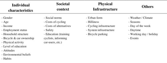
With 1.3 billion people, China is the most populous country in the world and the second largest land mass nation. High population densities observed in many Chinese cities and the growing motorization due to China’s economic expansion, both result in high traffic congestion, parking inefficiencies and environmental challenges. This has led to increased interest in sustainable transportation alternatives, such as bike-sharing, which refers to the supply of bicycles by companies to enable short-term rental to customers with the convenience of usage without the obligation of ownership (Shaheen, Guzman, and Zhang 2010). The demand of such bike-sharing services, however, is affected by a variety of factors. These factors range from individual characteristics (i.e. gender, age, income, etc.) over societal norms (i.e. policies) to physical infrastructure (i.e. local occurrences) and others (i.e. weather; Heinen, Wee, and Maat 2010).
Bike-sharing providers aim to understand underlying factors that drive customer behavior to tailor their service offerings to customer needs, for instance by accurately predicting demand and replenishing bikes at the right place and the right time to avoid stock-outs. Capturing information facilitating that purpose has become easier as technological advancements enabled bike-sharing service providers to equip bicycles with technologies that allow tracking bikes throughout the city (Chen and Storey 2012). The data generated by these systems is therefore attractive as the bike-sharing companies can gain further insights to adapt their services to the customer needs and habits (Fishman, Washington, and Haworth 2013).
1.1 Problem Definition
The sponsoring company of this research project, TalkingData, who is also China’s largest independent data platform, collects app-usage, location and sensor data after the agreement of the app developers from more than 750 million smart devices. TalkingData leverages this data by feeding it into their big data
system, aiming to provide insights that help companies to achieve a competitive advantage. Figure 1 illustrates TalkingData’s value proposition.
Figure 1: TalkingData's Value Proposition towards Companies
The large number of devices leads to over 20 terabytes of data to be collected and more than one billion session requests every day. As a result, TalkingData faces common big data challenges, such as that the information collected is not properly formatted to be easily analyzed, hence it is complex to obtain insights even if sufficient data exists (Labrinidis and Jagadish 2012). However, working with the collected data to identify drivers of bike-sharing demand and using advanced forecasting methods as tool to predict demand would allow TalkingData serving its clients interested in bike-sharing.
1.2 Project Objectives
The described problem prompted us taking up the challenge to analyze smartphone data to understand the bike-sharing demand in Beijing, which is the purpose of this study. We worked with TalkingData to:
• assess the adequacy of mobile data for generating insights into bike-sharing, • collect additional primary and secondary data and connect it with mobile data, • determine factors that drive bike-sharing demand in Beijing, and
• build predictive models for bike-sharing services in Beijing and evaluate their suitability for mobile data.
1.3 Report Outline
Following this chapter, Section 2 presents an introduction of bike-sharing as new transportation method as well as how new technologies affect and advanced statistical methods affect the same. Section 3 defines the research methodology for this project. Section 4 provides the analysis of the data and illustrates the results. Section 5 contains a comparison of the forecasting models. Finally, Section 6 presents the conclusions and proposes avenues scope for future research of this topic.
> 600 million
Mobile Devices TalkingData Clients
App-usage Location Data Sensor Data Insights Solutions Consulting
2. Literature Review
This section begins by illustrating the concept of bike-sharing and its current adaption in China as well as its capital Beijing. In addition, it is reflected how big data and its related business analytics can become a source for companies’ value creation to the customer. Lastly, some previous research with a similar project scope is discussed, focusing on the used methodology and the results achieved.
2.1 Bike-sharing as a new public transportation service
Bicycle usage offers a variety of advantages over other modes of transportation, thus, represents an attractive alternative for urban travels. At an individual level, cycling is a healthy and cheap form to commute, which even proves itself sometimes faster than other transport modes, especially in urban areas. At the same time, societies benefit from less pollution and noise, cheaper infrastructure and improvements in public health (Kalter 2007). However, bicycle usage requires a greater physical effort with lower speed than motorized transport. It also depends on reasonable weather conditions and makes it difficult to carry loads1. Prior research has identified a variety of determinants2 for the usage of bicycles and bike-sharing
systems. An overview is provided in Table 1.
Table 1: Overview of factors related to bicycle and bike-sharing usage Individual characteristics Societal context Physical Infrastructure Others - Gender - Age - Income - Employment status - Household structure - Bicycle & car ownership - Physical activity - Level of education - Attitudes - Environmental beliefs - Habits - Social norms - Costs of cycling - Costs of alternatives - Safety - Education (training cyclists, informing car-users, etc.) - Urban form - Hilliness - Cycling infrastructure - System infrastructure - Bicycle parking - Weather / Climate - Seasons
- Day of the week - Daytime
- Working day / holiday - Events
Source: Heinen, Wee, and Maat 2010
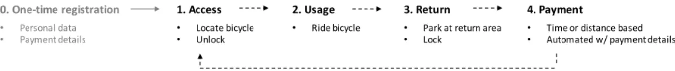
While providers differ in their nature (i.e. government bodies, transport agencies, etc.) mainly for-profit companies aim to leverage the described advantages and introduced bike-sharing systems as service of public transportation. Even though bike-sharing systems have existed for almost fifty years, they have grown significantly in prevalence and popularity within the recent years (Ricci 2015). During this time bike-sharing systems have progressed through four distinct stages, which are referred to as ‘generations’ in literature3 (DeMaio 2009; Shaheen, Guzman, and Zhang 2010). Current bike-sharing systems represent third generation systems: often incorporating IT-based systems that enable the access of the bicycle or to track bicycles utilizing GPS. Refer to Figure 2 for an illustration of the operating principles of a typical bike-sharing system.
Figure 2: Operating principle of bike-sharing system
After an initial registration, users can access available bikes and use them within the provider’s business area. Depending on the business model of the bike-sharing provider the bike is either returned at docks (station-based) or freely in the business area (free-floating). The process is completed with a time or distance travelled usage-based payment.
The ease of use of these systems combined with the general advantages of bicycle usage and the eliminated necessity of bicycle ownership led to a high demand in bike-sharing across the world. In accordance to that, China4 (and especially Beijing) experienced a tremendous boom in bike-sharing demand. It reached such
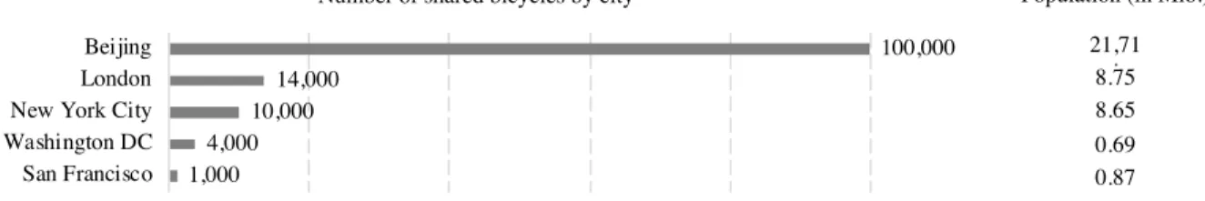
scale and is deeply embedded in the city transportation ecosystem, that providing the right number of bikes into the city at the right time is a great challenge for bike-sharing service providers. Figure 3 shows a
3 Refer to Shaheen, Guzman, and Zhang 2010 for an overview of components and characteristics of each generation. 4 Refer to Appendix A on page 36 for a brief introduction of China’s transport system.
1. Access • Locate bicycle • Unlock 2. Usage • Ride bicycle 3. Return • Park at return area • Lock 0. One-time registration • Personal data • Payment details 4. Payment • Time or distance based • Automated w/ payment details
comparison of major cities across the globe and their respective number of bicycles provided through bike-sharing systems.
Figure 3: Bike-sharing bicycles and population of major cities in the beginning of 2017 5
To improve urban mobility services, it is necessary to identify relationships between such demand and influencing factors (Wen, Sun, and Zhang 2014). Though, prior research often considers determinants independently from each other. It is not clear which are the factors that most strongly influence the usage. Fortunately, new technologies enabled through technical advancement provide the opportunity to look at several factors at the same time.
2.2 Big data, analytics and the path from raw data to insights for bike-sharing companies
The amount of data in the world has been exploding since networked sensors are embedded in mobile phones, automobiles, and other devices, enable them to sense, create and communicate data. These technological advancements allow companies to collect information about their environment (i.e. customer behavior, machinery conditions, etc.). According to Manyika et al. (2011) big data refers to datasets whose size is beyond a typical database and allows data to be captured, stored, managed, and analyzed. The promise of data-driven decision-making is now recognized broadly, both, from practitioners and researchers, leading to a growing enthusiasm for the notion of big data (Chen and Storey 2012).
Opportunities associated with big data, its analysis and analytics refer to the techniques, technologies, systems, practices, methodologies, and applications that analyze critical business data. The methods used are drawn from several fields including statistics, computer science, applied mathematics, and economics, leading to a multidisciplinary approach in helping decision makers to better understand their business and 5 https://www.ft.com/content/5efe95f6-0aeb-11e7-97d1-5e720a26771b 1,000 4,000 10,000 14,000 100,000 San Francisco Washington DC New York City London Beijing
Number of shared bicycles by city Population (in Mio.) 21,71
8.75 8.65 0.69 0.87
simplify the decision making (Manyika et al. 2011). Generating valuable insights from raw data involves multiple steps (Labrinidis and Jagadish 2012):
1. Acquire: Connect to data sources and collect data 2. Explore: Preview data to determine the potential
3. Transform: Enrich the data from other data sources and clean the dataset for analysis 4. Analyze: Question data using visual representations and statistical methods
5. Share insights: Provide information to stakeholders involved.
However, challenges arise at all phases of the analysis, such as heterogeneity, incompleteness, scale, timeliness and privacy of the data. Thus, leveraging big data in order to create value poses itself as a complex process, but is pursued by bike-sharing companies in order to advance from the third to the fourth generation of bike-sharing systems. Being driven by delivering a better service experience to the customer than the competition, companies aim to integrate smart management schemes into their bike-sharing systems. Hence, utilizing real-time and non-real-time big data about bikes and their environment to understand activity patterns and to predict demand, would allow companies to not only improve their services but also to offer new ones (Razzaque and Clarke 2015).
2.3 Methods and results of similar projects
Bike-sharing companies have the collective goal of meeting the needs of the final customer, by supplying bicycles at the right place, time and price (Helms, Ettkin, and Chapman 2000). Accurate and effective forecasting of future demand is essential for making supply chain decisions. Yet, the complexity and uncertainty existing around demand makes forecasting a challenge. Since customer demand is influenced by a variety of factors, understanding relationships between these factors and bike sharing demand would enable companies to improve the forecasts (Chopra and Meindl 2014). Due to its importance for companies’ success, other case studies related to bike-sharing demand forecasting already exist. We have summarized the most relevant studies in Table 2 with focus on the modeling methodologies, the valuation method and the results.
Table 2: Overview of similar demand forecasting case studies
Title Modeling Methodologies Valuation Conclusion
Forecasting Utilization in City Bike-Share Program (a)
(1) Neural Network (2) Poisson Regression (3) Markov Model (4) Mean Value Benchmark
RMSLE Neural Network is found to perform the best which is 0.49.
Predicting Capital Bikeshare Demand in R (b)
(1) Regression
(2) Generalized Boosted Models
RMSLE The GBM model clearly performed better than our linear regression model
Bike Share Demand Prediction using RandomForests (c)
(1) Random Forest
(2) Enhancing RM model using TuneRF (3) Conditional Inference Trees (4) Generalized Boosted Models
RMSLE Random Forest
with TuneRF performance is 0.49
Research on Antecedents and Consequences of Factors Affecting the Bike Sharing System (d)
(1) Multiple linear regression (2) Poisson and Topology method
P-Values Temperature that people feel is most important determinant
Forecasting Bike Rental Demand (e)
(1) Basic Linear Regression (2) Generalized Linear Models with Elastic Net Regularization (3) Generalized Boosted Models (4) Principal Component Regression (5) Support Vector Regression (6) Random Forest
(7) Conditional Inference Trees
RMSLE Two of the Tree based models are found to perform the best:
• CTree: 0.46 • Random Forest: 0.50
Demand Prediction of Bicycle Sharing Systems (f)
(1) Ridge Regression
(2) Support Vector Regression (3) Random Forest
(4) Gradient Boosted Tree
RMSLE Random forest is found to perform best
Bike Sharing Demand: Forecast use of a city bikeshare system (g)
(1) Gradient Boosted Decision Trees (GBDT)
RMSLE RMSLE value of GBDT Loop is 0.5683
Forecasting Bike Rental Demand Using New York Citi Bike Data (h)
(1) Linear Regression (2) Neural Network (3) Decision Tree (4) Random Forest
RMSLE Random forest model has shown relative best performance
Prediction of Bike Sharing Demand (i)
(1) SVM
(2) Neural Network (3) Poisson Regression (4) Random Forest (5) Extra Trees Regressor (6) GBM
(7) Linear Combination Model (8) Discriminating Linear Combination Model
RMSE Linear Combination model and Discriminating Linear Combination model are good models for predicting bike sharing demand with RMSE being close to 0.36
Legend: (a) Lee, Wang, and Wong 2014; (b) Liu 2015; (c) Patil, Musale, and Rao 2015; (d) Jing and Zhao 2015; (e) Du, He, and Zhechev
3. Methodology
This section first discusses the underlying research strategy. It is then presented in detail how to collect the qualitative and quantitative data required for the purpose of this research. Subsequently, the statistical approach for analyzing and visualizing the obtained data is illustrated. Finally, the used forecasting methods and the respective evaluation techniques are outlined.
3.1 Research Strategy
The objective of this research is to determine factors that drive bike-sharing demand in Beijing, recommend models to forecast the demand, apply these methods and evaluate their suitability for TalkingData’s data. To fulfill these objectives and get a holistic impression of the bike-sharing market in Beijing, we gather and analyze both, qualitative and quantitative data. We conduct interviews with key stakeholders and industry experts to get qualitative stakeholder opinions. At the same time, we compile a data set with the help of TalkingData and online resources enabling us to detect patterns about the bike-sharing usage. Lastly, we developed three forecasting models using different methods and tested their performance on the dataset.
3.2 Qualitative Data Collection and Analysis
As a consequence, this research includes both, qualitative and quantitative analysis and primary as well as secondary data needs to be collected. Since the data to be obtained differs in its nature, distinct collection methods are used, which are outlined in the following.
3.2.1 Conducting key stakeholder interviews
To gather insights from key stakeholders including bike sharing service providers, users and urban planners, a number of in-depth interviews are performed. The aim is to have a semi-structured, direct personal contact with the interviewee to uncover underlying motivations and beliefs towards bike-sharing (Harris 1996). The advantages are a great depth of insights and free exchange of information. However, a major challenge is that the data obtained is difficult to analyze after transcribing, as interviewees have their individual way of expressing themselves and interpret the context (Malhotra and Birks 2007). The qualitative interview
will be based upon a face to face conversation in which the emphasis of the research is to ask open ended questions and listening, so as to promote the interviewee to divulge as much information as possible in his answers (Kvale 1996). The degree of structure of the interview is semi-structured, yet the level of probing is high, in order to generate further explanation from the research interviewee. In this research, the following people are interviewed:
• two users from Beijing, to derive first opinions about drivers of the bike sharing demand • a city manager from Ofo, to gain insights into the perspective of bike-sharing providers
• a Senior urban researcher of the city of Beijing Municipal Planning Institute, to gain insights about bike sharing system from the perspective of urban planning.
The main objective is to examine their views on the most important usage drivers for bike share system. The questions center around the purpose of sharing bike usage, and the environmental, regulatory and marketing factors that would influence demand.
3.3 Quantitative Data Collection and Analysis
This section comprises of an explanation how we obtain a dataset that enables us to generate insights, as well as its exploration and the further analysis we perform using more advanced statistical models.
3.3.1 Data Sample
We worked with TalkingData to discover which data the company can provide which is consistent, suits the company’s computational power and enables us to deliver further insights. TalkingData provided us with data that presents the number of devices with active bike-sharing applications on the smartphone, indicating the demand during a certain period of time. However, this would only allow for time-series analysis. As the company is interested to answer questions such as: which impact weather or pollution has on demand, or how many bikes are rented on working days compared to the weekend. Therefore, we enriched the provided dataset by TalkingData with data from other online resources which enables us to
provide insights into the bike-sharing service in Beijing. We collected the following data and merged it with TalkingData’s data6:
1. Weather information (i.e. temperature, wind speed, etc.) 2. Air quality (i.e. pollution)
3. Holiday and working weekend (i.e. is respective day a holiday)
3.3.2 Data Exploration and Visualization
To understand the landscape of the data and discover initial patterns, we explore the data first. This includes various data aggregations and summaries, both numerically (e.g. correlation matrix) and graphically (e.g. boxplots, scatterplots, density plots). In this step, we are interested in both, looking at variables separately as well as looking at the relationships between the variables in order to generate some initial hypotheses.
3.3.3 Identification of Demand Drivers
To identify the main drivers of bike-sharing demand, given our dataset, we use multi linear regression models with the demand being the dependent variable and several independent variables (such as temperature, pollution, etc.). We chose the linear model, in order to identify the dependent variables linear dependency on the independent variables (i.e. the direct impact). To identify which factors influence the demand statistically significantly, the p-value (in different levels) is taken into account (*p<0.1, **p<0.05, ***p<0.01).
3.4 Building Forecasting Models
As identified in the literature review, several models can be fitted to forecast the bike-sharing demand. In this paper we use linear regression, neural networks and random forest. All of these represent supervised learning algorithms and allow for predicting a numerical value. This means that we fit a function based on pairs consisting of input (independent variables) and an output variable (dependent variable). The inferred function is then applied on new independent variables in order to predict the dependent variable. In the
optimal scenario, we would be able to forecast the exact demand of bike-sharing per hour. We fit and asses the performance of the models using three different approaches:
• we partition the data into training (75% of the data) and validation (25%) sets on a city level o we fit a model to the entire Beijing city using the training set, predict the demand of the
validation set, and calculate the RMSE (root mean squared error) to assess the performance • we partition the data into training (75% of the data) and validation (25%) sets on a district level
o we fit a model to every district in Beijing using the training data, predict the demand on the district level as well, aggregate the district forecasts and calculate the RMSE for the entire city
• we use 10-fold cross validation
o essentially, we take our city level dataset and split it into 10 groups, for each of the 10 groups, we train on the remaining 10−1 groups and validate the performance on the kth group
For the partitioning approach, we also plot histograms of the forecasting errors and visualize the real vs. predicted values. Based on the respective plots and the resulting RMSE we can assess the performance of the algorithms for the present data.
4. Interview and Data Sample Results
This section illustrates the results from the qualitative and quantitative data analysis. The section first highlights insights from the stakeholder interviews. Then the quantitative data is explored and the drivers for bike-sharing demand are determined. Finally, forecasting models for predicting the bike-sharing demand are fitted and their performance is compared.
4.1 Insights from Interviews
All interviewees believe sharing bikes in Beijing are mostly used for basic last-mile transit in areas that public transportation, such as metro, does not cover. Sharing bikes are considered as replacement of bus, walk, short-term taxi/ride-sharing, and illegal auto-rickshaw. Entertainment and fitness purposes also exist, but only account for very small portion of total usage.
In the interviews, we have discovered a few insights that were commonly identified by all three types of stakeholders. Extreme temperature in the winter and summer is considered the most crucial factors driving bike-sharing demand. Service providers collect 2/3 of all bikes back to warehouses in November and distribute bikes back to the city only in March, as they expect a seasonal drop of demand. Wind and rain would also significantly reduce the usage. Both the interviewees from service provider and urban research institute think that pollution, which is commonly measured by Chinese users in PM2.5, does not affect sharing bike usage. However, both of the two user interviewees claimed they would not use bike-sharing if the air quality is bad. In addition, the urban researcher and service provider interviewees have suggested other drivers. Regulation on the supply of new bikes and the city infrastructure such as bike lanes would affect the overall usage of sharing bike within a city. The service provider believed that promotion and price reduction also significantly drives the usage. In contrast, the users claim that they rather have a strong brand preference, therefore this would might not be a main concern for them7.
4.2 Exploratory Analysis
Overall TalkingData provided us with 1,215,894 single observations over a period of one month (11pm on 05/28/2017 to 9am 06/25/2017). A data point is assumed to be obtained at the beginning of the trip (i.e. representing the departure with a bike).
4.2.1 Location and Time
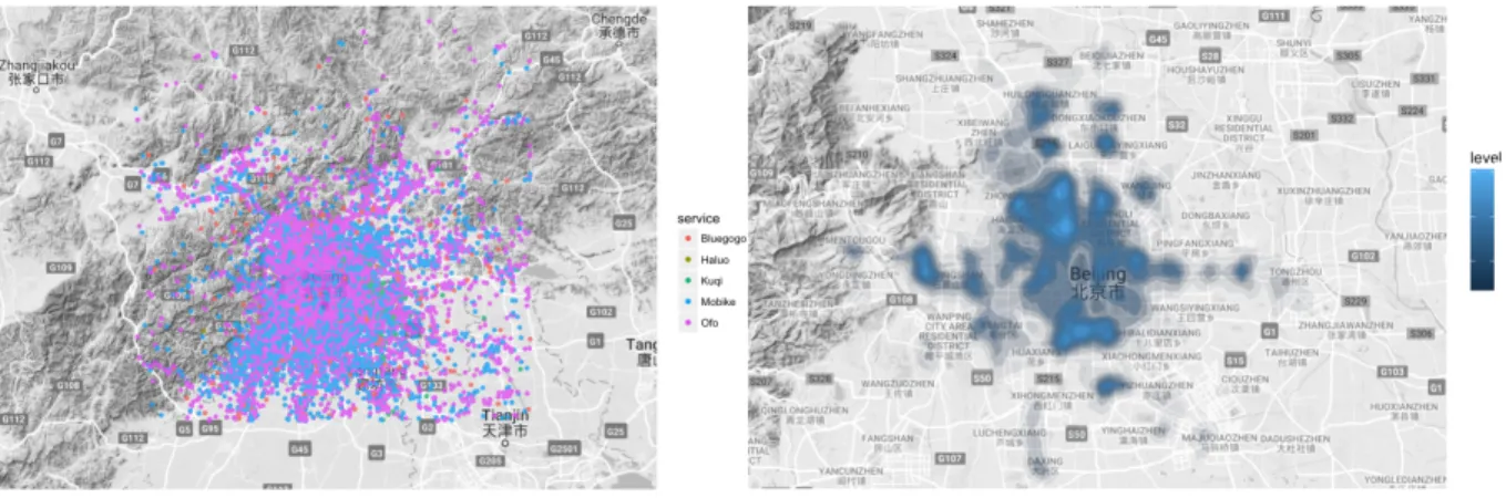
To get a first impression of the data, we mapped the observations using the respective longitude and latitude data, while also getting a first glimpse on the density of the demand (Figure 4). We have data from five different bike-sharing service providers (Bluegogo, Haluo, Kuqi, Mobike and Ofo) which are marked by different colors as you can see in the legend. The observations are spread over an area of 115.4175 to 117.4999 (longitude) and 49.43011 to 41.03888 (latitude), hence representing a vertical spread of ~177km and a horizontal spread of about ~179 km.
Figure 4: Plot all observations and demand density
The left part of Figure 4 illustrates that the data obtained is manly derived from the two bike-sharing companies Ofo (pink) and Mobike (blue). These companies are the largest bike-sharing service providers in Beijing. The right part of Figure 4 illustrates the demand density of all observation, in which a higher level (illustrated by a brighter color) represents a greater level of activity, or in other words, more demand. We notice that some areas experience greater demand than others (i.e. the observation density is higher in certain regions). Even though some demand derives from the outskirts of Beijing, TalkingData is specifically interested in the city center of Beijing, due to a greater activity level. Beijing’s landmass is
characterized by a public transportation system that includes train lines surrounding the city. We look at the bike-sharing demand in Beijing in greater detail, by narrowing down the scope to the first three rings of the city. Figure 5 provides an overview of both, the observations per ring (left) as well as the bike-sharing demand density within this area. The inner ring (red) represents an area of about 66 km2, the second ring (green) includes an area of about 99 km2 (excluding the inner ring) and the area of the third ring (blue) is about 176 km2 (outer ring only).
Figure 5: Observations per city ring and demand density in Beijing city center8
It seems that within the area inside the three rings, two regions (north-west and mid-south) experience the greatest demand. As a next step, we identified whether this demand pattern is constant or changes over the day. From Figure 6 we see three exemplary demand density plots (5am, 11am and 9pm). We see that the demand is fluctuating across the area throughout the day9.
5 am 11 am 9 pm
Figure 6: Exemplary demand density at 5am, 11am and 9pm
8 i.e. area within the three first rings
9 Please refer to Appendix E on Page 39-40 for a hourly demand density overview.
While it seems that in the early morning a great demand is located in the south of Beijing, it transitions towards the north just before noon while two main demand locations (north and south) co-exist in the evening. Hence, both the location and the time of the day seem to drive bike-sharing demand.
Next, we analyze the relation between time and demand in greater detail. The scatterplot and boxplot in Figure 7 illustrate the demand per hour throughout the day.
Figure 7: Scatterplot and boxplot of demand per hour
While the bike-sharing demand in Beijing seems generally low between 0am and 5am it increases in the early morning hours before reaching its first peak between 9am and 10am. After slowing down a bit after noon, the second peak of the day is typically between 6pm and 8pm in the evening. Thus, we infer that the bike-sharing service tends to be used as part of the transportation system going to and leaving from work during the rush hours in the morning and evening. Additionally, we can see that the variability amongst the hours differs (i.e. very small demand variability in the morning compared to a greater demand variability during the rush hours). This means that forecasting the demand in the night-early early morning hours might be easier, than throughout the day.
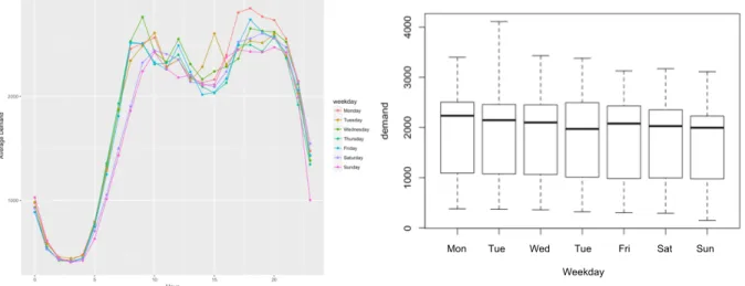
Figure 8 illustrates the average demand per hour of each respective weekday (left), in which each colored line represents a different day) and a boxplot of the demand per day of the week (right). We see that the rush hour pattern seems to replicate throughout all days of the week. One could have hypothesized that the bike-sharing demand pattern might differ between working days and weekends, yet this cannot be
confirmed. However, the bike-sharing demand peaks during the weekend (Saturday and Sunday as purple and pink lines) happens a bit later than during the work days (Monday – Friday). Additionally, the demand peaks in both the morning and evening is smaller in magnitude during the weekend (meaning that the demand is more even throughout the daytime at weekends).
Figure 8: Average demand per hour per day and boxplot of demand per day
The boxplot indicates that the bike-sharing demand seems to be quite constant throughout the week, as the median demand per day differs only slightly. Taking Figure 9 into account we see that the bike-sharing service tends to be used a bit less during the weekend, as both the median demand and the interquartile range is lower on the weekend. Thus, we could argue, that the bike-sharing service is more used during the week in order to reach or leave the workplace rather than for leisure. Additionally, we observe a greater demand variability during the week, which might be the result from more days being included in the week.
Figure 9: Boxplot demand weekend and holiday
Mon Tue Wed Tue Fri Sat Sun
After exploring location and time as potential drivers of bike-sharing demand, we find that there is a lot of variability still unexplained. This means that there need to be other factors beyond location and time that can explain other parts of the bike-sharing demand variability. Thus, in the following section, the impact of environmental factors on the bike-sharing demand is assessed further.
4.2.2 Environmental Conditions
Figure 10 shows scatterplots of the bike-sharing demand per hour given external conditions, such as temperature, humidity, or wind speed. Here, darker colors present a greater density meaning that the frequency of hourly bike-sharing demand is greater during that particular environmental condition.
Figure 10: Scatterplots environmental conditions and demand as # of bike trips within an hour
It seems that the higher the temperature the greater tends to be the bike-sharing demand. In contrast, with an increasing dewpoint, an increasing humidity or and increasing air pressure the bike-sharing demand
seems to decrease. Both wind speed and air quality seem to not impact bike-sharing demand significantly. Though, these findings are based on the visual illustrations of the respective relationships where it is difficult to draw upon a statistical significance. Figure 11 illustrates the correlation amongst these environmental factors including demand.
Figure 11: Correlation matrix environmental factors and demand
We see that demand is positively correlated with the temperature and wind speed, but negatively correlated with the dewpoint, humidity and lightly with pressure. The air quality, however, tends to be uncorrelated with demand. Other noticeable correlations are temperature and humidity (highly negative, i.e. the higher the temperature, the less humid it is), humidity and dewpoint (highly positive, i.e. when a high humidity is observed on could also except a high dewpoint), as well as temperature and wind speed (highly positive). However, correlation does not necessarily indicate causation. In order to derive insights on which factors significantly drive the bike-sharing demand and investigate the relationships amongst the variables further, we ran various regression models. In other words, we use linear regression models to identify which factors from our data set cause an increased or decreased bike-sharing demand.
4.3 Bike-sharing Demand Drivers
Similarly, to our exploratory analysis, we first look into the impact of time, followed by the impact of environmental conditions.
4.3.1 Time Regression Models
We first created a new variable dayperiod which indicates whether it is night (omitted, 10pm – 5am), morning (6am – 12pm), afternoon (1pm – 5pm), or evening (6pm – 9pm). Our first model includes all time-related factors (except weekend1 due to singularity means, i.e. not linearly independent). Since dayperiod seems to be highly significant, we account for dayperiod throughout our other regression models and observe the relationships of other variables on bike-sharing demand by adding them separately.
Table 3: Time regression models
Dependent variable: Demand (1) (2) (3) (4) (5) dayperiodmorning 1,253.000*** 1,254.000*** 1,253.000*** 1,253.000*** 1,253.000*** (48.120) (48.260) (48.160) (48.100) (48.290) dayperiodafternoon 1,384.000*** 1,385.000*** 1,384.000*** 1,384.000*** 1,384.000*** (53.010) (53.170) (53.060) (52.990) (53.200) dayperiodevening 1,677.000*** 1,678.000*** 1,678.000*** 1,678.000*** 1,678.000*** (56.950) (57.120) (57.010) (56.920) (57.150) weekdayMonday 206.500*** 177.400** (73.510) (70.970) weekdayTuesday 162.800** 133.700* (73.510) (70.970) weekdayWednesday 149.700** 150.900** (70.910) (70.970) weekdayThursday 77.550 78.800 (70.910) (70.970) weekdayFriday 98.400 99.640 (70.910) (70.970) weekdaySaturday 56.650 57.900 (70.910) (70.970) weekend1 -99.290** (41.960) pubhol -121.400 -41.940 (80.980) (73.320) Constant 776.600*** 874.300*** 775.000*** 903.000*** 877.400*** (56.630) (32.930) (56.670) (34.980) (33.410) Observations 673 673 673 673 673 R2 0.658 0.653 0.657 0.656 0.653 Adjusted R2 0.653 0.651 0.653 0.654 0.651 Residual Std. Error 492.500 (df = 662) 493.900 (df = 669) 492.900 (df = 663) 492.200 (df = 668) 494.200 (df = 668) F Statistic 127.600*** (df = 10; 662) 419.100*** (df = 3; 669) 141.200*** (df = 9; 663) 317.900*** (df = 4; 668) 314.100*** (df = 4; 668) Note: *p<0.1; **p<0.05; ***p<0.01
Similar to our findings earlier, Models (1) - (5) suggest that the time of the day is a significant driver for bike-sharing demand, as all periods of the day are highly significant. In contrast, only the demand on Monday, Tuesday and Wednesday is significantly different compared to the omitted day (Sunday, Model (3)). We have sufficient evidence to suggest that the bike-sharing service is used significantly less during the weekend compared to weekdays (Model (4)). Model (5) indicates that demand for bike-sharing decreases during public holiday (negative coefficient), though this is not significant. Hence, we have more evidence to suggest that bikes are particularly used as transportation to and away from work.
4.3.2 Environmentally Conditions Regression Models
In Model (6), we included several environmentally related factors from our dataset10. Temperature and pressure are the only factors that are highly significant. In the following models, we control for temperature and investigate the relationships of other variables on bike-sharing demand by adding them separately.
Table 4: Environmental regression models
Dependent variable: Demand (6) (7) (8) (9) (10) (11) temp 76.3*** 73.7*** 54.1*** 88.2*** 68.0*** 75.0*** (10.0) (4.9) (7.6) (5.5) (5.8) (5.0) humidty -193.0 -596.0*** (194.0) (177.0) pressure 37.8*** 39.9*** (8.2) (7.4) windspeed 11.3* 11.2* (5.9) (5.9) airqual -2.0 -2.4 (1.5) (1.5) Constant -38,040.0*** -7.2 759.0*** -40,553.0*** 22.4 53.4 (8,429.0) (125.0) (259.0) (7,559.0) (126.0) (130.0) Observations 671 673 673 671 673 673 R2 0.3 0.2 0.3 0.3 0.3 0.3 Adjusted R2 0.3 0.2 0.3 0.3 0.3 0.2 Residual Std. Error 709.0 (df = 665) 726.0 (df = 671) 720.0 (df = 670) 712.0 (df = 668) 724.0 (df = 670) 725.0 (df = 670) F Statistic 54.0*** (df = 5; 665) 222.0*** (df = 1; 671) 118.0*** (df = 2; 670) 130.0*** (df = 2; 668) 113.0*** (df = 2; 670) 112.0*** (df = 2; 670) Note: *p<0.1; **p<0.05; ***p<0.01
From Model (6) – (11) we see that temperature has a positive impact on the bike-sharing demand – the higher the temperature the higher the demand. However, this can be misleading as with increasing temperature at some point taking a bike might not be pleasant for some people anymore. Therefore, it is interesting to investigate whether the impact on bike-sharing demand is actually linear or rather polynomial. Model (8) illustrates that with increasing humidity (on a scale from 0 to 1) the demand for bike-sharing is decreasing. Model (9) and (10) highlight that both increasing pressure and increasing wind speed cause a greater bike-sharing demand. Just as the factor temperature, these respective relationships require further investigation. Surprisingly, according to Model (11), the air quality has no significant on the bike-sharing demand. Naturally one would expect a decrease in demand with a worsening air quality, but we do not have enough evidence to suggest a significant relationship.
As mentioned earlier, the variables temperature, pressure and wind speed require some further investigation. It is analyzed whether these variables tend to have a linear or polynomial relationship on the outcome variable bike-sharing demand. First, two new temperature variables are created (temp2 and temp3). Model (13) is the regression model in which temp and temp2 are regressed on the bike-sharing demand. Similarly to model (13), in Model (14) temp3 is added as well. The linear and quadratic relationships towards bike-sharing demand are illustrated in the graph, and present the findings graphically.
Table 5: Temperature regression models
Dependent variable: Demand (12) (13) (14) temp 73.70*** 268.00*** -212.00 (4.95) (39.50) (213.00) temptemp -3.77*** 15.40* (0.76) (8.39) temptemptemp -0.25** (0.11) Constant -7.23 -2,383.00*** 1,470.00 (125.00) (495.00) (1,752.00) Observations 673 673 673 R2 0.25 0.27 0.28 Adjusted R2 0.25 0.27 0.28 Residual Std. Error 726.00 (df = 671) 713.00 (df = 670) 711.00 (df = 669) F Statistic 222.00*** (df = 1; 671) 127.00*** (df = 2; 670) 87.00*** (df = 3; 669)
Note: *p<0.1; **p<0.05; ***p<0.01 Figure 12: Plot temperature and demand
We see that in Model (13) all coefficients are statistically significant (in Model (14) they are not), indicating a quadratic relationship. This means that one more degree leads to a greater increase in bike-sharing demand when the temperature is low compared to when the temperature is already higher11. We see that at a temperature of about 33°C and greater the bike-sharing demand reaches a point where an increasing temperature decreases the bike-sharing demand.
The same approach is utilized to investigate the relationship between wind speed and bike-sharing demand.
Table 6: Wind speed regression models
Dependent variable: Demand (15) (16) (17) windspeed 47.10*** 89.30*** 78.60 (5.52) (18.50) (51.50) windwind -1.61** -0.75 (0.68) (3.96) windwindwind -0.02 (0.09) Constant 1,340.00*** 1,130.00*** 1,164.00*** (62.70) (108.00) (188.00) Observations 673 673 673 R2 0.10 0.11 0.11 Adjusted R2 0.10 0.10 0.10 Residual Std. Error 795.00 (df = 671) 792.00 (df = 670) 793.00 (df = 669) F Statistic 72.90*** (df = 1; 671) 39.60*** (df = 2; 670) 26.40*** (df = 3; 669) Note: *p<0.1; **p<0.05; ***p<0.01
From Model (16) we see that the relationship is quadratic as well, so that with excessive wind-speed the bike-sharing demand decreases. Figure 13 reveals that the tipping point is at about 25 km/h.
We also analyzed the underlying relationship between pressure and bike-sharing demand. However, our analysis showed a polynomial relationship with more than five degrees. Thus, due to its complexity and potential overfit, we retain pressure as linear coefficient.
11 Since our dataset represents a sample of the real data it not meaningful to interpret the absolute value of the slope differences. Thus, in our work the relative observation matters more, however, in future work we recommend TalkingData to analyze this relationship in greater detail.
Figure 13: Plot wind speed and demand
4.4 Discussions
To summarize this chapter, we compare our qualitative and quantitative insights. From both the interviews and the bike-sharing demand data set we find that extreme temperatures have an impact of bike-sharing demand, so that a very high temperature lowers the bike-sharing demand. We obtained similar findings for wind and rain. Interviewees as well as the data show that with increasing wind speed and rain (humidity) the demand significantly decreases.
Interestingly, we do not obtain consistent results for air quality (pollution). While employees of the sharing service providers and the urban researcher state that the level of pollution would not affect bike-sharing demand. In contrast, bike-bike-sharing users indicate that they would not use the service in case of bad air quality. From the data, we retain the hypothesis that pollution is not affecting bike-sharing demand. Hence, either the interviewed bike-sharing users are not representative for the entire set of bike-sharing users, or people believe that they would not use the service in case of a bad air quality, but are unaware when the pollution level rises.
After better understanding the drivers of bike-sharing demand in Beijing by comparing the insights generated from both, interviews and quantitative analysis, we now focus on forecasting models as tools to predict bike-sharing demand in Beijing.
5. Forecasting Models
Based on our literature review we fit basic models of regression, neural network and random forest to the dataset provided by TalkingData, as these models were frequently used in similar studies. We aim to test the three different forecasting techniques utilizing insights generated in the previous chapter, to provide a comparison of how accurate the models work with TalkingData’s data.
To get a more reliable comparison, we fit the models using two different procedures. On the one hand, we fit the models on all observations within the three rings (i.e. the area indicated earlier), forecast the demand and compare it with actual numbers. On the other hand, we divide the area in the seven city districts Chaoyang, Chongwen, Dongcheng, Fengtai, Haidian, Xicheng and Xuanwu. We then fit the models to each respective district, forecast the demand in each, merge the results and compare it with actual numbers. Figure 14 illustrates the observations of the seven districts of Beijing we take into account.
Figure 14: Observations per city district
The reasoning is that districts in Beijing differ by certain characteristics such as industry focus, economic activity and demographics. Hence, a more specific model could better be better at predicting the demand in the respective district resulting in being more accurately. We fit the models and compare their accuracy using data set partitioning (i.e. training and validation set, both on district and city level) and k-fold cross validation (on city level).
5.1 Regression
For the regression model, we use bike sharing demand as dependent variable and hour, weekday, temperature, temperature2, humidity, pressure, wind speed, wind speed2 and air quality as independent variables. Figure 15 shows the histogram of the forecasting errors both for the regression on district level (and aggregation afterwards) and on city level.
Figure 15: Histogram regression forecasting errors
We see that the errors are almost normally distributed around zero (i.e. the perfect estimation). Figure 15 shows the real observations in comparison to the predicted values by the fitted regression forecasting model, both on district and city level. The line indicates the actual value of bike-sharing demand, whereas the dots present the prediction.
Figure 16 indicates the exact same forecasting performance for the district level and city level model. This is confirmed by the RMSE, which is 133.51 for both models. This results from the linearity of the regression model and the constant predictor matrix (i.e. the independent variables are the same amongst all districts as well as across the entire city, as only our dependent variable changes). However, this results only holds if the predictor matrix is constant. In contrast, using the 10-fold cross validation approach we reach an RMSE of 138.93, which means that the 10-fold cross validation approach performs slightly worse compared to the partitioning approach.
5.2 Neural Network
For the neural network, we pre-process the data and scale the numerical predictors and the outcome variable to a 0-1 scale. We also convert the categorical predictors to dummies. We then use bike-sharing demand as outcome variable and 34 inputs as a result of our pre-processing (factors, etc.). We fitted several different neural networks with the varying layers and nodes to the data. We start taking the rule of thumb into account which says that the optimal size of hidden layers is usually between the size of the input and the size of the output. We find that reducing the number of nodes leads to a better performance, ultimately ending up using 2 nodes and 1 hidden layer as best fit. Figure 17 shows the histogram of the forecasting errors both for the neural network applied on district level and on city level.
The histograms indicate that both on district and city level most of the errors are negative, which means that most of the predictions are underestimated. Figure 18 shows the real observations in comparison to the predicted values by the fitted regression forecasting model, both on district and city level.
Figure 18: Neural network forecast vs real observations
After de-normalization, we reach a RMSE of 176.99 using the district level and a RMSE of 153.03 on the city level. Thus, the neural network seems to perform better on city level. Using the 10-fold cross validation approach we reach an RMSE of 221.38, performing worst amongst the neural network models12.
5.3 Random Forest
We build a basic random forest model using the same dependent and independent variables as in the regression model. In regard to the number of trees, the default tree number of random forest is 500. Figure 19 shows the random forest performance in terms of error for a varying number of trees included.
Figure 19: Random forest performance per number of trees
We see that when the tree number is greater than 75, the line (i.e. error) becomes more stable, and when bigger than 350, the error is very stable. Thus, we set the tree number (ntree) to 350 in this project.
Figure 20 shows the histogram of the forecasting errors both for the random forest model applied on district level and on city level.
Figure 20: Histogram random forest forecasting errors
Similarly to the linear regression model, we observe an almost normal distribution of the errors around 0. Figure 21 shows the real observations in comparison to the predicted values by the fitted random forest forecasting model, both on district and city level.
Even though the random forest model is based on regression decision trees, we need to state that the decision trees are not linear. This is why we obtain a different performance on district and city level. The RMSE of the district random forest model is 146.28, while the city level random forest model results in a RMSE of 138.64. In contrast, using the 10-fold cross validation approach for the random forest model we reach an RMSE of 143.5213.
5.4 Comparison of Forecasting Models
To better be able to compare the models, we plot the predicted values of the linear regression, neural network and random forest model in comparison to each other in Figure 22 and Figure 23. Observations on (or close to) the line indicate a good prediction.
Figure 22: Forecast vs. real observations comparison - district
Figure 23: Forecast vs. real observations comparison - city
We can see that the neural network seems to perform worst amongst the respective models. The performance difference between the linear regression and random forest models seem to be less. Both of them show a distribution of predicted values and observations which are to some extent comparable to a “line”, meaning they tend to be more accurate than the neural network. It is noticeable that the extreme values (i.e. higher demand) are predicted less accurately across all forecasting models.
To further address which model performs most accurate, the RMSE of the partitioning models (both district and city level) and the cross-validation models are taken into account (Table 7).
Table 7: Forecasting models’ RMSE summary
Fitting Approach
Algorithm District Level City Level Cross Validation
Linear Regression 133.51 133.51 138.93
Neural Network 176.99 153.03 221.38
Random Forest 146.28 138.64 143.52
Our data set has a demand observation range of 3957 (i.e. max hourly demand 4109 – min hourly demand 152) and an average demand per hour of 1807. The RMSE is then one standard deviation of the deviation of our predictions from the actual value. Comparing the RMSE to the mean and range, we see that all of the models seem to provide meaningful value in terms of predictive performance, as the size of the RMSE is comparably small across all forecasting models (range of 7.4% - 12.3% of the mean).
As already indicated, the RMSE of both the regression and random forest are smaller than the RMSE of the neural networks. However, we can also see that the regression model performs best. Usually one would expect the cross-validation to perform best. The worse performance in this case could result from the initial seed for the data partitioning. The seed and the resulting 75:25 partition seems to be working well, especially across the city-level models. However, even though the CV-RMSE is greater across all models compared to the partition models, the ranking amongst them is equal to the single models (i.e. the linear regression cross validation performs best, random forest second and neural network third). Hence, the regression model would be recommended for further use as a forecasting model based on the data at hand.
However, the models are fitted with a relatively small number of observations (in terms of sufficiency for machine learning algorithms). While the regression model works comparably best in the current setting, we expect the performance of random forest and neural networks to increase when fitted on a larger dataset (for instance twelve months of data). Therefore, we recommend using regression to forecast the demand when only a small data set is available, whereas it would be valuable to further analyze the performance of other models such as neural networks and random forest if the data set available is larger.
6. Conclusion
In response to increasing urbanization, China’s central government is encouraging alternative public transportation methods, such as bike-sharing, which has demonstrated social and environmental benefits. As a result, interest in bike-sharing has increased so that the number of bike-sharing programs has grown rapidly over the last five years in China. Whilst bike-sharing providers have undoubtedly enhanced user convenience and reduced travel time, an opportunity for providers exists to enhance bike sharing’s performance by understanding customer needs and behavior, for instance through leveraging data collected during trips, about the user demographics as well as about external conditions.
Our sponsoring company TalkingData aims to provide insights to bike-sharing service providers in order to improve the level of service for bike-sharing users. Therefore, our main objective in this project was to analyze smartphone data to understand the bike-sharing demand in Beijing. We conducted interviews with bike-sharing stakeholders and investigated a one-month sample of data that TalkingData collected from bike-sharing operators in Beijing merging it with secondary data from online resources. We created a dataset allowing for determining underlying factors that drive bike-sharing demand and fitting forecasting models to predict the number of bike-sharing rental demand based on based aspects such as, day of the week, time, weather, temperature, etc.
We found that the level of bike-sharing activity varies across the city Beijing and throughout the day. We discovered that both, time related factors such as time of the day or weekend as well as environmental related factors such as temperature, humidity or wind speed, significantly affect the bike-sharing demand. In contrast, our study revealed that some factors stated in literature and revealed during interviews with bike-sharing users such as air quality or pollution level does not significantly affect bike-sharing demand in Beijing. Hence, we suggest that drivers of bike-sharing demand differ across cities or countries making it worthwhile to perform location specific analysis.
Based upon reviewing available literature on bike-share services and predictive modelling algorithms we fitted linear regressions, neural networks and random forests on the compiled dataset and compared their respective performance. We found that based on the one-month sample linear regression performs best amongst the three models in predicting hourly bike-sharing demand in Beijing, irrespective of whether the prediction is performed on a city or district level. However, in terms of data sufficiency for building machine learning models, our dataset tends to be small. We assume that including more data would result in greater performances of neural network and random forest algorithms.
It needs to be noted, that the insights we derived only result from one month of data (extracted from TalkingData’s platform). In order to gain more robust results, the time-frame of the data should be extended (e.g. 1 year or 2 years of data). It would be possible to gain an understanding on the impact of seasonality, growth development, etc. Our analysis on demand drivers also could be run on specific districts or only for certain bike-sharing service providers to see whether they differ from the average Beijing customer, so that both districts and bike-sharing service providers could better understand the demand drivers of their respective area or customer base.
Additionally, to gain further insights on the individual behavior, the dataset could be enriched with personal information, such as age, sex or new vs. old users. This would allow to further segment the customer base and target customers more specifically. Another possibility would be to add further variables to the model that are more holistic, such as gasoline price or government policies. Since the car-sharing follows the free-floating principle, one could map specific locations such as public transport stations, etc. and find their impact on personal behavior.
Bibliography
Chen, Hsinchun, and Veda C Storey. 2012. “Business Intelligence and Analytics : From Big Data To Big Impact”. Mis Quarterly 36 (4): 1165–88.
Chopra, Sunil, and Peter Meindl. 2014. Supply chain management: strategy, planning, and operation. Igarss 2014. Pearson.
DeMaio, Paul. 2009. “Bike-sharing : History , Impacts , Models of Provision , and Future”. Journal of Public Transportation 12 (4): 41–56.
Du, Jimmy, Rolland He, and Zhivko Zhechev. 2014. “Forecasting Bike Rental Demand”. Fishman, Elliot, Simon Washington, and Narelle Haworth. 2013. “Bike share: a synthesis of the
literature”. Transport reviews 33 (2): 148–65.
Harris, Leslie M. 1996. “Expanding horizons”. Marketing Research 8 (2): 12.
Heinen, Eva, Bert Van Wee, and Kees Maat. 2010. “Commuting by Bicycle : An Overview of the Literature”. Transport Reviews: A Transnational Transdisciplinary Journal 30 (1): 59–96.
Helms, Marilyn M., Lawrence P. Ettkin, and Sharon Chapman. 2000. “supply chain management Supply chain forecasting”. Business Process Management Journal 6 (5): 392–407.
Hua, Shaoyang, Junli Wang, and Yin Zhu. 2013. “Cause Analysis and Countermeasures of Beijing City Congestion”. Procedia - Social and Behavioral Sciences 96 (Cictp). Elsevier B.V.: 1426–32. Jing, Chen, and Zuoyuan Zhao. 2015. “Research on Antecedents and Consequences of Factors Affecting
the Bike Sharing System”. In International Conference on Logistics Engineering, Management and Computer Science, 444–49.
Kalter, MJ Olde. 2007. More often the bicycle? Effects of government measures. Kennisinstituut voor Mobiliteitsbeleid. Den Haag.
Kvale, Steinar. 1996. An Introduction to Qualitative Research Interviewing by Steinar Kvale .
Labrinidis, Alexandros, and Hosagrahar V. Jagadish. 2012. “Challenges and opportunities with big data”. In Proceedings of the VLDB Endowment, 5:2032–33.
Lee, Christina, David Wang, and Adeline Wong. 2014. “Forecasting Utilization in City Bike-Share Program”.
Liu, Rongfang, and Chang-Qian Guan. 2005. “Mode Biases of Urban Transportation Policies in China and Their Implications”. Journal of Urban Planning and Development 131 (2): 58–70.
Liu, Wayne. 2015. “Predicting Capital Bikeshare Demand in R”.
Malhotra, Naresh K, and David F Birks. 2007. Marketing Research: An Applied Approach. World Wide Web Internet And Web Information Systems. 3rd ed. Vol. 3. Financial Times Prentice Hall.
Manyika, James, Michael Chui, Brad Brown, Jacuqes Bughin, Richard Dobbs, Charles Roxburgh, and Angela Hung Byers. 2011. “Big data: The next frontier for innovation, competition, and


![[PDF] Formation générale en pdf de VBA | Cours informatique](data:image/gif;base64,R0lGODlhAQABAIAAAP///wAAACH5BAEAAAAALAAAAAABAAEAAAICRAEAOw==)