Tree growth forces and wood properties

HAL Id: hal-02984734

https://hal.archives-ouvertes.fr/hal-02984734v2

HAL is a multi-disciplinary open access archive for the deposit and dissemination of sci-entific research documents, whether they are pub-lished or not. The documents may come from teaching and research institutions in France or abroad, or from public or private research centers.

L’archive ouverte pluridisciplinaire HAL, est destinée au dépôt et à la diffusion de documents scientifiques de niveau recherche, publiés ou non, émanant des établissements d’enseignement et de recherche français ou étrangers, des laboratoires publics ou privés.

Tree growth forces and wood properties

Bernard Thibaut, Joseph Gril

To cite this version:

Article submitted to PCI Forest and wood sciences - 1st revision

Tree growth forces and wood properties

Running title: Tree growth forces Bernard Thibaut (1,*)_{, Joseph Gril} (2,3)

(1) _{LMGC, Univ Montpellier, CNRS, Montpellier, France - bernard.thibaut@umontpellier.fr} (*) _{Corresponding author}

(2) _{Université Clermont Auvergne, CNRS, Sigma Clermont, Institut Pascal, Clermont-Ferrand,} France

(3) _{Université Clermont Auvergne, INRAE, PIAF, Clermont Ferrand, France}

Highlight

Based on an experimental study of growth strains in trees restoring their verticality after accidental inclination, combined with measurements of wood properties at the same position, a method is proposed to reconstitute the history of growth force generation by the living wood.

Abstract

Living wood in the tree performs a muscular action by generating forces at sapwood periphery and residual strains in dead sapwood fibres. Dissymmetric force generation around tree trunk is the motor system allowing movement, posture control and tree reshaping after accidents. Rather young trees are able to restore the verticality of their trunk after accidental rotation of the soil-root system due to wind or landslide, leading to typically curved stems shape. The very high dissymmetry of forces for the motor action is associated with the occurrence of reaction wood on one side of the inclined stem during many successive years. A method to reconstitute this biomechanical history from observations after tree felling, on either green or dry wood, is discussed.

A selection of 17 such trees coming from 15 different species (13 different families), tropical or temperate, hardwoods or softwoods, were selected and peripheral residual strains were measured in situ before felling, on 8 position for each stem. Matched wooden rods were sawn and measured for their mechanical and physical properties at green and dry states, allowing the estimation of tree growth stress, i.e., the force created by the living wood. It was possible to build easy-to-use conversion coefficients between growth stress indicator (GSI), measured in situ by the single hole method, and growth strain and growth stress with the knowledge of basic density and green longitudinal elastic modulus.

Maturation strain, specific modulus (as a proxy of micro-fibril angle) and longitudinal shrinkage are properties independent from basic density, whose variation among species was very large. On the whole range of compression wood, normal wood and tension wood strong relationships between these 3 properties were observed, but altogether no single model based on cell-wall microfibril angle only could be used.

Growth forces are the product of 4 parameters: ring width, basic density, basic specific modulus and maturation strain, all of them being the result of wood formation. Thanks to the wide range of wood types and species, simple and highly significant formulas were obtained

for the relationship between basic and dry density, green and dry longitudinal modulus of elasticity, basic and dry specific modulus. To estimate ring width in green state from values in dry state, radial shrinkage needs to be measured afterwards on dry specimens. Maturation strains is less accurately linked to late measurements on dry wood, but longitudinal shrinkage offers a rather good solution for an estimation provided that the wood type (softwood, hardwood with-G layer, hardwood without G-Layer) is known.

Keywords

Force generation; growth strains; modulus of elasticity; wood shrinkage; tree biomechanics; wood

Abbreviations and notations

NW, RW, OW normal wood, reaction wood, opposite wood TW, CW tension wood, compression wood

MFA mean microfibril angle relative to L direction

 density

, Dg, BD, DD density, green density, basic density, air-dry density MOE, E, EL modulus of elasticity in L direction

Eg, Ed green, air-dry MOE

G, GTL, GRL shear modulus

k factor for shear contribution (5/6 for rectangular cross section)

SM specific modulus (MOE divided by density)

SMb basic SM (MOE divided by basic density)

EL/ SM in L direction

EL/GTL, EL/GRL anisotropy factor GSI growth stress indicator

m maturation strain

 conversion factor m /GSI

m (initial or peripheral) maturation stress

 conversion factor m /GSI

F growth force

L, R, T longitudinal, radial, tangential directions 𝐿k, Rk, Tk dimension in L, R, T direction for condition k

M mass

DPx distance to pith

RH relative humidity

MC, MCg, MCd wood moisture content, in green condition, in air-dry condition VS, LS volumetric, longitudinal shrinkage

FSP fibre saturation point

Introduction

During the beginning of this 21st _{century much has been done and written about the} biomechanics of force and stress generation resulting from wood growth, after the 20th century had been more dedicated to large measuring campaigns of wood properties to encompass their very large variability. Wood tissues fulfil several functions in the tree: tree

growth, sap ascent, mechanical resistance to external forces, storage of water and numerous organic or mineral components, communication between tree parts and the roots. During tree life, wood growth and properties adapt to tree environment so as to regulate each function in conjunction with the others. Consequently, wood variability results both from genetic speciation and from physiological adaption during the process of wood formation. Many studies dedicated to the hydraulic function link variations of wood structure and properties of different species to changes in water availability and, conversely, predict climatic variations using variations in wood structure and properties. Could the same be done with biomechanical functions? Assuming that they are successfully linked to wood growth, structure and property, would it be possible to read in wood specimens the trace of tree biomechanical history?

Basics of tree biomechanics

The study of the residual stress resulting from tree growth started in the late 1920ties_{. It was} mostly measured at trunk periphery and its effects during the early stages of wood processing, such as end splitting of felled logs or warping of sawn timber, were described (Gril et al 2017). Models of stress distribution within a trunk were proposed (Archer 1986, Kubler 1987, Fournier et al 1991a, 1991b, Alméras et al 2018a).

Since the beginning of the years 2000the biological origin and function of large peripheral residual stress has been thoroughly investigated by experimental work at cell wall level together with biomechanical models of stress generation within wood fibres. From the mechanical viewpoint wood fulfils three basic functions in the tree: achievement of tree architecture (manufacturing), control of axis direction (posture control), resistance to external forces (resistance) (Alméras et al 2009, Tocquard et al 2014, Thibaut 2019).

The following paragraphs give a synthetic overview of many results, often published in recent books or review articles cited in priority to avoid lengthy lists of references.

Wood growth in mass and volume

All wooden parts of a tree are slender beams (axis) clamped at the proximal end (junction). Such cantilever beams can be vertical (trunk), oblique or horizontal. Each axis is made of a succession of primary growth units (Barthélémy & Caraglio 2007), result of the division of stem cells in primary meristems (buds). A portion of growth unit, between junctions, has the shape of a multi-layered cylinder with an inner skeleton of mostly dead fibre cells and pipe elements, a thin layer of living cells, with a nucleus and a cytoplasm, and an outer bark layer (Fahn 1990). Wood formation, its growth in volume and mass, occurs through a 3D manufacturing process taking place in the thin intermediate living layer. At the cellular level the process requires three steps: cell division, cell expansion until final geometry, cell-wall thickening (maturation) until programmed cell death and full cell-wall lignification (Thibaut 2019). At the plant level it consists in axis lengthening by addition of new growth units and thickening of existing parts by addition of a new peripheral layer thickness. The mass increment all along the axis produce an increase of gravity forces and moments, together with an increase of sectional area and moment of inertia. The distribution of mechanical stress resulting from this manufacturing and the action of gravity (self-weight) is called support stress (Fournier et al 1991a). It vanishes at periphery where the new wood was just deposited.

The generation of maturation forces

During cell-wall thickening and maturation, the newly formed wood fibres generate growth forces (Alméras & Clair 2016). The basic process of force generation is a small contraction or dilatation of the cell-wall polymer network. At the tissue level the resulting expansion is restrained by the rigid wood skeleton (Alméras et al 2018a). When the maturation process is completed, the so-called maturation strain (m) has been produced, while the longitudinal

elastic modulus has reached a stable level (EL) and the initial maturation stress is set up as

their product:

m = EL . m

Considering a layer portion of the newly formed wood of sectional area A, the growth force generated by the incremental wood growth in the longitudinal direction is:

F = A . m = A . EL . m

During each growth event, the local force generated by the cell maturation depends on ring width, wood elastic modulus and maturation strain. As a reaction to the effect of maturation in the newly formed wood layer, a counteracting stress is induced in the existing stem. The cumulative stress distribution resulting from the maturation process only, independently from gravity, is called the maturation stress.

Residual or growth stresses: pre-stressing of the skeleton

The total stress due to wood growth, called growth stress, is the sum of support stress and maturation stress (Fournier et al 1991b). The peripheral support stress being equal to zero, the peripheral stress equals the initial maturation stress m. In an ideal tree growing with

perfect symmetry, ring width, EL and m are the same all along the circumference. Since wood

strength in L direction is more than two times higher in tension than compression (Markwardt and Wilson 1935) the resulting uniform tensile pre-stressing at periphery enhances the resistance to bending (Gordon 1978, Gril et al 2017) which is the most dangerous situation for slender beams.

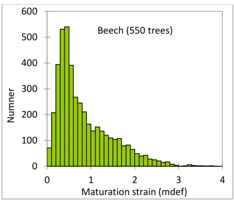
The growth stress can be estimated by different methods using strain gauges or strain transducers, measuring the strain associated to the stress release (Yoshida and Okuyama 2002, Yang et al 2005, Clair et al 2013, Gril et al 2017). It has been usually observed at sapwood periphery of standing trees, at different angular position and a given height level, but measurements of the internal distribution of residual stress were also performed through successive cutting and strain acquisitions. To obtain the local maturation force generated by a portion of recently formed wood, the measurement of the area (e.g., ring width) and elastic modulus is also needed. Numerous measurements on many trees have been performed in different contexts (Sasaki et al 1978, Okuyama et al 1994, Huang et al 2001, Alméras et al 2005b, Ruelle et al 2007, Jullien et al 2013). There is a clear difference between softwoods and hardwoods. For hardwoods, maturation strains are always associated to tensile maturation forces with a long tail of very high values, up to 5 times the most common value (Fig. 1). For softwoods on the contrary there is a tail associated to compressive values (Fournier et al 1994). Mean standard strain values (around 0.05%) are associated to tensile stress for hardwoods (HW) and softwoods (SW).

Species is not a significant factor in the variations of m. The most important factor is always

Tree slenderness is also a significant factor for the mean maturation strain between trees: very slender trees have a higher mean level within a species (Jullien et al 2013). These slender trees have also a higher elastic modulus (Waghorn et al 2007, Watt et al 2008, Moore et al 2015) so that slender trees exhibit much higher m - but not always high Fm because of their

narrow rings.

Fig. 1 - Distribution of maturation strains for 550 beech trees (Becker and Beimgraben 2001); mdef: 1/1000.

Normal wood and reaction wood

Reaction wood (RW), either tension wood (TW) or compression wood (CW) were identified in the 1970ties as the origin of the peculiar values of m, very high tensile or compressive,

respectively (Boyd 1972, Trénard and Guéneau 1975, Timell 1986, Okuyama et al 1994, Bamber 2001). A rather recent book “Biology of reaction wood” (Gardiner et al 2014) gives a state of the art concerning tension and compression wood for anatomy (Ruelle 2014), cell-wall polymers (Fagerstedt et al 2014), molecular mechanisms of induction (Tocquard et al 2014), biomechanical action (Fournier et al 2014), physical and mechanical properties (Clair & Thibaut 2014). Most of recent developments were dedicated to TW. A new distinction is made between pure G-layer fibres, multi-layered G-fibres, late lignified G-fibres and no G-fibres (Ghislain & Clair 2017, Higaki et al 2020). Further observations and model were discussed about cellulose within the G-layer (Chang et al 2015, Alméras & Clair 2016, Gorshkowa et al 2018) with a relative consensus about a lattice structure of cellulose microfibrils in the G-layer. Each wood species has a given pattern (signature) in sapwood anatomy and chemistry of the cell wall polymers: percentage of each basic polymer (cellulose, lignin, different types of hemicellulose) and H, G, S monomer proportions within the lignin. Normal wood (NW) is the most abundant wood type in a tree and both anatomy and chemistry have only small variations around the specific patterns. RW is triggered by specific genes and both their anatomical and chemical features differed markedly from the mean patterns (Table 1).

0

100

200

300

400

500

600

0

1

2

3

4

N

u

m

n

er

Maturation strain (mdef)

Beech (550 trees)

Associated variations in physical and mechanical properties differ between CW and TW as compared to NW. Basic density is always higher for CW in a given tree but the difference is often not significant for TW. Specific modulus of elasticity, which is very strongly linked to the microfibril angle (Cowdrey & Preston 1966, Cave & Hutt 1968), is always very low for CW and always high for TW, but for NW it can vary from very low for very juvenile wood to very high for resonant wood (Brémaud et al 2013). The total longitudinal shrinkage, always very low for NW (below 0.4%), is much higher for CW (up to 4%) and for TW (up to 1.5%).

Table 1 - Variations in structure and chemistry for normal and reaction wood Wood type Anatomy MFA Lignin

chemistry Cellulose chemistry Hemicellulose chemistry Normal wood (softwood) Standard anatomy 5° - 40° Lignin content 25%- 38% 40% - 60%

Low 6 carbon sugar % High 5 carbon sugars % Normal

wood (hardwood)

Standard

anatomy 5° - 40° 16% - 41% 28% - 58%

High 5 carbon sugars % Low 6 carbon sugar % Compression wood Round tracheids 30° - 50° 5 to 10% higher high H/G 5 to 10% lower smaller fibril width Higher galactose content Tension wood Often G-layer fibres 0° - 15° 5 to 10% lower high S/G 5 to 10% higher larger fibril width

Globally similar except for G-layer MFA: mean microfibril angle

Posture control by maturation forces dissymmetry

The primary function of force generation is the motor action for posture control of the slender wooden stem (Moulia et al 2019, Fournier et al 2013). Vertical growth is an unstable process: any small accidental rotation of the root system, or pruning of a lateral branch, results in a small trunk inclination and sligthly oblique growth, that would rapidly diverge to high levels without a rapid counteracting action. Oblique growth, on the other hand, is very common for branches or the shoots of a coppice. Length and mass increase of the stem cause increment of bending moment supported by the wooden cross section, leading to an increase of stem slope which needs to be actively counteracted through the generation of an opposite moment all along the stem (Alméras et al 2018a). This motor action is obtained by a dissymmetry of Fm

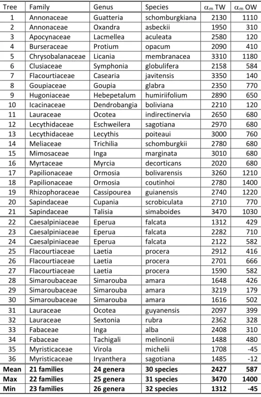
between upper and lower part of the stem. In the case of an accidentally inclined trunk, a higher-than-usual motor action is needed until it recovers verticality (Coutand et al 2007, Moulia & Fournier 2009). In this case, RW is used on one side of the stem during all the process of verticality restoration while the opposite wood (OW) formed on the other side is similar to NW (Table 2).

Nearly always, there is a kind of pseudo-sinusoidal variation of m. around the periphery of

the trunk (Alméras et al 2005b, Ruelle et al 2011, Jullien et al 2013), even when there is no value indicating RW. In this case the difference between upper and lower face values is much lower (See Annex 1 for beech and chestnut). When the active counter action needed for oblique growing is not too high (small trunk inclination), variations of m within NW,

associated with eccentric growth, are enough: both “tensile” and “opposite” sides are NW. For oblique growing with higher inclination (as for many branches) and fast restoration of verticality, the use of RW is necessary (Yoshida et al 2000).

Table 2 - Maturation strain (in µdef) for various trees restoring their verticality in French Guiana

Tree Family Genus Species m TW m OW

1 Annonaceae Guatteria schomburgkiana 2130 1110

2 Annonaceae Oxandra asbeckii 1950 310

3 Apocynaceae Lacmellea aculeata 2580 120

4 Burseraceae Protium opacum 2090 410

5 Chrysobalanaceae Licania membranacea 3310 1180 6 Clusiaceae Symphonia globulifera 2158 584 7 Flacourtiaceae Casearia javitensis 3350 140

8 Goupiaceae Goupia glabra 2350 770

9 Hugoniaceae Hebepetalum humiriifolium 2890 650 10 Icacinaceae Dendrobangia boliviana 2210 120 11 Lauraceae Ocotea indirectinervia 2650 680 12 Lecythidaceae Eschweilera sagotiana 2970 680 13 Lecythidaceae Lecythis poiteaui 3000 760 14 Meliaceae Trichilia schomburgkii 2780 680

15 Mimosaceae Inga marginata 3010 680

16 Myrtaceae Myrcia decorticans 2020 680

17 Papilionaceae Ormosia bolivarensis 3260 1210 18 Papilionaceae Ormosia coutinhoi 2780 1400 19 Rhizophoraceae Cassipourea guianensis 2740 1220 20 Sapindaceae Cupania scrobiculata 2710 770 21 Sapindaceae Talisia simaboides 3470 1030

22 Caesalpiniaceae Eperua falcata 1312 429

23 Caesalpiniaceae Eperua falcata 2282 710

24 Caesalpiniaceae Eperua falcata 2122 582

25 Flacourtiaceae Laetia procera 2912 416

26 Flacourtiaceae Laetia procera 2701 666

27 Flacourtiaceae Laetia procera 1590 582

28 Simaroubaceae Simarouba amara 1648 426

29 Simaroubaceae Simarouba amara 3219 179

30 Simaroubaceae Simarouba amara 1616 502

31 Lauraceae Ocotea guyanensis 2097 399

32 Lauraceae Sextonia rubra 2362 328

33 Fabaceae Inga alba 2408 310

34 Fabaceae Tachigali melinonii 1488 480

35 Myristicaceae Virola michelii 1708 -45

36 Myristicaceae Iryanthera sagotiana 1485 -12

Mean 21 families 24 genera 30 species 2427 587

Max 22 families 25 genera 31 species 3470 1400

Min 23 families 26 genera 32 species 1312 -45

Tree 1 to 21: data from Clair et al 2006; tree 22 to 30: data from Ruelle et al 2011; tree 31 to 36: data from Chang et al 2009. Negative values correspond to compression stress

Material and methods

Selection of standing trees

On the basis of the experimental campaigns conducted so far in 2001 it appeared that the main source of variation of m was the mechanical adaption of the tree to requirements of

difference was found between species; however, the diversity of studied species was not so high. In order to observe a wider diversity of species, 11 trees were selected in a tropical rain forest of French Guiana with the help of the botanical expert M.F. Prévost, each from a different family - one tree per species and one species per family. Three poplar trees and three conifer trees (spruce and pines) from temperate forest in France and China were added to the sampling in order to widen the selection (Table 3). For the spruce tree, two logs, corresponding to two GSI measurement levels (see below), where used, at 1m distance from each other. The objective was not to obtain a mean value or a range of values per species or family for biomechanical parameters such as m, but to investigate the links between maturation forces

and wood properties, with the hypothesis that each measurement point is representative of wood maturation.

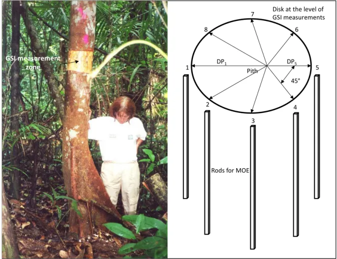
Rather young trees exhibiting a common type of bottom geometry with a basal curvature where chosen (Fig. 2). Young trees are more efficient in restoring verticality; they have been selected to have a sufficient thickness of reaction wood in the upper or lower part of the trunk, just above the curvature. The diameter at breast height of the 17 trees did not exceed 40cm and the mean was 26.4.

Table 3 - Trees used in the study

Family Genus Species DBH RW

Melastomataceae Miconia fragilis 23.6 GL

Meliaceae Carapa procera 23.4 GL.

Lecythidaceae Eschweilera decolorens 23.8 LGL Vochysiaceae Qualea rosea 30.3 LGL Cecropiaceae Cecropia sciadophylla 25.3 GL Lauraceae Ocotea guyanensis 30.9 GL. Flacouritaceae Laetia procera 29.4 GLc. Bignonaceae Jacaranda copaïa 21.7 NGL Myristiceceae Virola surinamensis 20.4 NGL. Cesalpinaceae Eperua falcata 27.9 GL. Simaroubaceae Simaruba amara 27.7 NGL.

Salicaceae Populus hybrid 38.3 GL

Salicaceae Populus hybrid 34.8 GL

Salicaceae Populus hybrid 25.4 GL

Pinaceae Picea abies 24.9 CW

Pinaceae Picea abies 24.9 CW

Pinaceae Pinus pinaster 20.1 CW

Pinaceae Pinus sylvestris 23 CW

Mean 26.43

DBH: diameter at breast height of the trees in cm

RW, reaction wood type (from Ghislain & Clair 2017): GL= tension wood (TW) with gelatinous layer, LGL = TW with a lignified G layer, GLc= TW with a multilayer G layer, NGL= TW with no G layer,

CW= compression wood

In situ measurements of maturation strain

The single-hole method developed in CIRAD (French agricultural research and international cooperation organization) was used. Two pins are inserted in the trunk surface in longitudinal

alignment 45mm from each other (Jullien et al 2013). This distance is measured with a linear displacement transducer before and after drilling a hole of diameter 20mm and depth about 20mm in the middle between the two pins. The difference in µm between after and before drilling is called growth stress indicator (GSI); it is positive for a tension force and negative for a compression force. Eight GSI measurements are performed on each tree or tree level, equally spaced around the circumference, beginning by the top of the inclined trunk for hardwoods, where TW is expected, or by the bottom for softwoods, where CW is expected.

GSI is theoretically (Archer 1984) related to maturation strain (m) by the relationship: m =  . GSI, m in microstrain (µ = 10-6), GSI in µm,  in µ/µm

where the calibration factor  is calculated by modelling the drilling of an anisotropic material occupying a half plane, though a complex equation using wood elastic constants and geometrical factors (distance between pins and hole diameter), see Annex 2.

Fig. 2 - Tree measured in French Guiana, wooden disk and rods sawn for each tree DPx: distance to pith from the x GSI point

Wood specimens for physical and mechanical properties measurements.

Just after cutting each tree, a disk (2cm thick) was crosscut at the level of GSI measurements (Fig. 2). Distance from pith to bark (DPx) for each GSI measurement position was measured.

Eight longitudinally oriented rods where sawn just above the disk, at the 8 GSI positions, the closest possible to the bark, few days after tree felling, in local workshop. The dimensions of the rods were 500mm (L, longitudinal direction) x 25mm (R, radial direction) x 25mm (T,

Pith 1 2 3 4 5 6 7 8 DP1 DP5 45°

Disk at the level of GSI measurements

Rods for MOE

GSI measurement zone

tangential direction) and they were kept in green state, wrapped in food-grade transparent cellophane, until the measurement of green MOE (Eg). A total of 144 rods were prepared.

A smaller rod (50mm x 25 mm x 25 mm) was cut from theses long rods for shrinkage study after Eg measurement.

The remaining long rods (430mm x 25 mm x 25mm) were air dried in the conditioned chamber at 65 % air relative humidity (RH) and 20°C temperature until equilibrium, corresponding to wood moisture content (MC) around 13%. The MOE was again measured on the air-dry rods as such, giving a “crude” air-dry MOE. Rods were then planed on four sides to get standard air-dry rods (400mm x 20mm x 20mm) and standard air-dry MOE (Ed) was measured again. Modulus of elasticity

The flexure free-free vibration method analysed with Timoshenko model (Bordonné 1989, Brancheriau & Baillères 2002) was used for all measurements. Dimensions in the 3 directions (L, R, T) and mass (M) of the rods were measured with a good precision (0.1%). The rod was put on 2 thin wires at the positions of first vibration mode nodes and tapped at one end, successively on the radial (TL) and tangential (RL) face, corresponding to the RL and TL hitting plane, respectively. The resonant frequency fi was measured for the three first vibration

modes (f1, f2, f3). Using the approximate solution of free vibration theory of Timoshenko,

Bordonné (1989) proved that two useful variables xi and yi can be built from fi frequencies,

theoretically linked by the expression:

yi = E/ - xi . E / (k.G)

where E is the longitudinal modulus of elasticity (MOE) of the rod, G the shear modulus in the hitting plane (GTL or GRL, depending on the orientation of the rod on the wires),  the rod

density and k a fixed factor. The 3 frequencies (f1, f2, f3) give 3 points of coordinates (xi, yi)

allowing to fit the equation of a straight line with a regression coefficient that should be very close to 1.0. The slope, the most sensitive to defects, and the intercept of the regression line are -E/(k.G) and E/ respectively E/ is the specific modulus (SM) and equals the square of sound speed in L direction (unit m²/s²) while the ratio E/G (EL/GTL or EL/GRL) describes elastic

anisotropy and is useful for the calculation of . Density is calculated as mass to volume ratio  = M/(L.R.T) and MOE by the formula E = SM.. Then G can be derived from E and E/k.G, with

k=5/6 for this geometry (Brancheriau & Baillères 2002). For some samples measurements with

regression coefficient below 0.98, the values for GTL or GRL were not considered.

Due to viscoelastic nature of wood and the smaller measurement times involved, the dynamic modulus obtained using vibration method is expected to be higher than the quasi-static modulus that would be more appropriate to analyse GSI measurements performed within a few minutes. It is, however, very well correlated and proportional to the quasi-static modulus obtained in 4 points bending, with a relative difference of only 4% (Brancheriau & Baillères 2002).

Maturation stresses

The peripheral maturation stresses (m) is calculated as the product of m and green MOE (Eg). Basic density and shrinkage measurements.

For each small rod, mass (M), volume (V) and longitudinal dimension (L) were measured at green state (Mg, Vg, Lg) and at anhydrous state (M0, V0, L0). From these values basic density (BD), volumetric shrinkage (VS) and longitudinal shrinkage (LS) were calculated as follows:

BD = M0 / Vg

VS= (Vg - V0) / V0

LS= (Lg - L0) / L0

Anatomical observations

On 2 selected positions on the two sides of the tree, anatomical observations were performed (Ruelle 2003). Anatomical sections (15 μm thickness) were cut on a microtome (Leitz with feather knifes) in the central zone of a shrinkage specimen. They were stained with a double coloration safranin/alcian-blue. Lignified cell walls have a red colour while pure cellulosic G-layers have a blue colour. Sections were observed with a light microscope (Olympus BX60) and pictures were taken with a digital camera (Nikon Coolpix 4500) with good definition (pixel density: 2272 x 1704) and a magnification factor of 100. A higher magnification factor (500) was used to measure micro-fibril angles for softwood species (Senft & Bendtsen 1985).

Results

Relationships between green and dry properties

Concerning the green state, MCg was on average 89%, ranging from 38% to 182% (39% to

155% as tree average) and was strongly dependent on wood density. The air-dry state, here, refers to the condition of the specimens after a long storage in a room controlled for temperature (T = 21°C) and air relative humidity (RH = 65%). The corresponding equilibrium MC (MCd) ranged from 12% to 16% depending on the species and wood type within the

species.

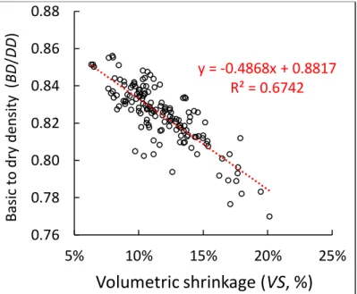
A proportional relationship, with a very high coefficient of determination, was observed between BD and air-dry density (DD) for this sampling (Fig. 3). The proportionality coefficient (BD/DD) had a mean of 0.826, very similar to the result of Vieilledent et al (2018) and ranged from 0.77 to 0.86. It depended mainly on the total volumetric shrinkage (VS) (Fig. 4).

Fig. 3 - Proportional relationship between dry and basic density

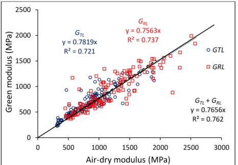
For MOE (E), specific modulus (SM) and shear moduli (GTL and GRL), there are also proportional

relationships between green and dry values. The determination coefficient (R²) is very high for

y = 0.8259x R² = 0.9996

200

400

600

800

1000

200

400

600

800

1000

B

asi

c

d

en

si

ty

(

BD

, k

g/

m

3

)

Dry Density (DD, kg/m3)

BD = f(DD)

E and SM (Fig. 5) and the influence of MC is relatively small (around 10% decrease from

air-dry to green state).

Fig. 4 - Dependence of the basic to dry density ratio on the total volumetric shrinkage.

Fig. 5 - Proportional relationship between air-dry and green values for longitudinal MOE (E, GPa) and specific modulus (SM, Mm²/s²); Eg: green MOE; Ed: dry MOE; SMb: basic SM; SMd: dry SM.

In the case of shear moduli, the proportional relationship is the same for the two directions (TL and RL) with a lower R², mostly due to the much higher sensibility of E/G (where G stands for either GTL or GRL) to small heterogeneities along the rod (Fig. 6). MC influence is higher

(around 25% decrease from dry to green state).

y = -0.4868x + 0.8817 R² = 0.6742 0.76 0.78 0.80 0.82 0.84 0.86 0.88 5% 10% 15% 20% 25% B as ic to dry den sit y (BD /DD )

Volumetric shrinkage (VS, %)

E

or

SM

E

or SM

E

SM

Fig. 6 - Proportional relationship between air-dry and green shear moduli

Calibration factor for maturation strains

The calibration factor can be calculated using the regression found in Annex 2 for all positions where EL/GTL is available at the green state:

 = -7.57 . Ln(ELg/GTLg) + 34.665

There was a very good exponential relationship between EL/GTL and basic specific modulus

(SMb), for all positions (Fig. 7).

Fig. 7 - Relationship between EL/GTL and basic specific modulus (SMb)

Using this exponential formula in the equation for the calibration factor , we find a linear relationship between  and SMb:

 (SMb) = -0.475 . SMb + 25.24 GTL y = 0.7819x R² = 0.721 GRL y = 0.7563x R² = 0.737 GTL+ GRL y = 0.7656x R² = 0.762 0 500 1000 1500 2000 2500 0 500 1000 1500 2000 2500 3000 G reen m o d u lu s (MP a)

Air-dry modulus (MPa)

GTL GRL y = 3.4711e0.0628x R² = 0.80 0 5 10 15 20 25 30 35 40 45 50 0 5 10 15 20 25 30 35 40 45 Rat io EL /G TL in g ree n s tat e

with the same regression factor (R² = 0.80). Considering that SMb is more easily and more

precisely measured, we have decided to use this relationship for the calibration factor figuring in the data sheet.

Peripheral maturation stress and GSI within a tree

In the first sheet of the accompanying Excel file named “Data_Tree_growth_forces”, tree-by-tree graphs are drawn showing the relationship between GSI and m for each tree. For each

tree there are 8 pairs of GSI - m measurements, yielding a proportional relationship with a

very high R² level (all R²>0.97 and 72% of R² values >0.99). This result suggests that it is perfectly suitable to use GSI as a proxy for m at tree level for biomechanics studies. The

conversion factor =m/GSI (in MPa/µm) ranged from 0.064 to 0.259 depending on the

species (Table 4).

Table 4 - Mean values of parameters per tree

Genus Species BD SMb Eg  R² Miconia fragilis 0.71 26.92 19.0 0.232 0.9997 Carapa procera 0.61 24.87 15.2 0.203 0.9941 Eschweilera decolorens 0.78 25.92 20.2 0.259 0.9996 Qualea rosea 0.56 21.29 12.1 0.199 0.9936 Cecropia sciadophylla 0.35 34.95 12.3 0.107 0.9788 Ocotea guyanensis 0.46 27.20 12.7 0.156 0.9903 Laetia procera 0.66 21.97 14.4 0.218 0.9979 Jacaranda copaïa 0.42 22.14 9.2 0.132 0.9916 Virola surinamensis 0.29 36.89 10.8 0.084 0.9954 Eperua falcata 0.70 22.99 16.1 0.234 0.9975 Simaruba amara 0.30 28.40 8.4 0.096 0.9976 Populus hybrid 0.29 28.04 8.2 0.110 0.9724 Populus hybrid 0.34 29.19 9.8 0.114 0.9903 Populus hybrid 0.38 19.37 7.4 0.128 0.9823 Picea abies 0.51 20.61 10.0 0.152 0.9933 Picea abies 0.49 18.10 8.4 0.142 0.9989 Pinus pinaster 0.42 10.68 11.4 0.064 0.9793 Pinus sylvestris 0.45 15.88 4.1 0.108 0.9882 BD: basic density (Kg/dm3_{); SM}

b: basic specific modulus (Mm²/s²); Eg: green elastic modulus (GPa);

: conversion coefficient for maturation stress (in MPa/µm); R² regression coefficient of the proportional relationship between m and GSI within the tree.

Force generation and longitudinal wood properties

The initial or peripheral maturation stress m is the force created by the living wood per unit

surface. It is the product of the maturation strain (m) and the green L MOE (Eg), itself the

product of BD and SMb. BD, SMb and m are the parameters resulting from the activity of the

living wood until fibre death.

A correlation analysis (Table 5) shows that m is mostly dependent on m (R²=88%) then on SMb (22%) and on BD (8%). Moreover, the three parameters SMb, Eg/GTLg, Eg/GRLg are very

Table 5- Correlation (Spearman) coefficients between parameters. m m BD SMb LS Eg GTLgg GRLg EL/GTLg EL/GRLg m 1 0.941 0.095 0.381 0.196 0.435 -0.049 -0.047 0.431 0.422 m *** 1 0.290 0.467 0.137 0.685 0.059 0.058 0.559 0.495 BD *** 1 -0.346 0.196 0.593 0.790 0.783 -0.094 -0.178 SMb *** *** *** 1 -0.189 0.500 -0.499 -0.508 0.843 0.828 LS * * * 1 -0.074 0.271 0.277 -0.231 -0.175 Eg *** *** *** *** 1 0.289 0.255 0.619 0.534 GTLg *** *** ** *** 1 0.866 -0.516 -0.473 GRLg *** *** ** ** *** 1 -0.421 -0.587 EL/GTLg *** *** *** ** *** *** *** 1 0.877 EL/GRLg *** *** * *** * *** *** *** *** 1

Bold characters: correlation significant at 0.001

***: correlation significant at 0.001 correlation significant at 0.01 *: correlation significant at 0.05

m: maturation strain; m: maturation stress;  and : conversion coefficients between GSI and

maturation strain and stress, respectively; BD: basic density (anhydrous mass/green volume); LS: total longitudinal shrinkage; Eg: green longitudinal elastic modulus; GTLg and GRLg: green TL and RL

shear modulus, respectively; SMb: basic specific modulus (green longitudinal elastic modulus/basic

density); Eg/GTLg and Eg/GRLg: anisotropy ratio in green condition in TL and RL plane, respectively.

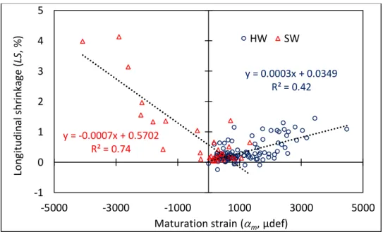
The correlation between LS and m is weak when all species are considered. This is not true

when putting apart hardwoods and softwoods (Fig. 8).

Fig. 8 - Relationships between longitudinal shrinkage (LS) and maturation strain (m)

HW: hardwoods; SW: softwoods

For each tree the angular variation around the perimeter of m and LS, in order to visualize

their relationships at the same position, is also given in the annexed Excel file. Globally, there is a clear association between zones with high and low level of each parameter. Tree by tree, the peak value (maximum in absolute value) is rather narrow and there is often an angular shift between m and LS which are not exactly measured at the same position. This explains

y = 0.0003x + 0.0349 R² = 0.42 y = -0.0007x + 0.5702 R² = 0.74 -1 0 1 2 3 4 5 -5000 -3000 -1000 1000 3000 5000 Lo n gi tu d in al s h ri n ka ge ( LS , % )

Maturation strain (m, µdef)

LS vs. am

why, besides the high similitude between profiles of the two parameters, regression coefficients (R²) are not so high (Fig. 8).

In order to have a global look on the parallelism between both variations, a “mean hardwood tree” and a “mean softwood tree” were calculated using the average of all hardwoods and all softwoods for m and LS (Fig. 9).

Fig. 9 - Circumferential variations for hardwoods (top) and softwoods (bottom)

am, LS: mean value for all trees at the angle position, of maturation strain and longitudinal shrinkage, respectively. Angle: angular position of the 8 measurement (degree). The angular position was shifted (+225°) in order to have the suspected reaction wood position in the middle of the profile These figures highlight the great similitude between maturation shrinkage (m) and

hygroscopic shrinkage in the L direction (LS) for hardwoods. For softwoods high shrinkage is associated to negative m. A very high similitude is found when using absolute values of m

(Fig. 10).

Fig. 10 - Circumferential variations for softwoods using absolute values for maturation strain. Same legend as Fig. 9

0 250 500 750 1000 1250 1500 1750 2000 2250 0 45 90 135 180 225 270 315 360 405 St rai n ( µ d ef ) Circumferential angle (°) Hardwoods am LS/3 -2500 -2000 -1500 -1000-500 0 500 1000 1500 2000 2500 0 45 90 135 180 225 270 315 360 405 St rai n (µ def ) Circumferential angle (°) Softwoods am LS/10 0 500 1000 1500 2000 2500 0 45 90 135 180 225 270 315 360 405 A b so lu te st rai n ( µ d ef ) Circumferential angle (°) Softwoods Abs(am) LS/10

Specific behaviour of reaction wood

Maturation strain values, longitudinal shrinkage of the associated rods, together with visual observation of the wood disks for softwoods (Fig. 11), allowed affecting a wood type to each tested specimen: 1=CW, 2=both CW and NW, 3=NW, 4=both NW and TW, 5=TW. Wood types 2 and 4 were attributed to rods containing both RW and NW. Transverse sections 15µm thick cut from two NW and two TW rods were used to examine wood anatomy (Fig. 12 and Fig.13).

Fig. 11 - Image of the section of Pinus pinaster tree with the positions of measurements CW: compression wood, OW: opposite wood, LW lateral wood

The mean microfibril angle (MFA) was measured for the conifer specimens only (Brémaud et al 2013). It is always high for CW, and globaly lower for NW but with some overlap around 30-35°. The trees were rather young (Fig. 11) so most of the NW can be considered as juvenile wood.

CW sector

Pinus pinaster

Positions of GSI measurements Rods for properties

measurement

OW sector LW sector

Fig. 12 - Comparative anatomy of compression wood (CW) and normal wood (NW) for the conifer species

For hardwoods, a majority of G-layer type TW (3 poplars, Miconia, Carapa, Ocotea, Cecropia, Eperua) were studied (Table 3), two species had a lignified G layer (Eschweilera & Qualea), one a peculiar multi-layered G layer (Laetia) and three no G layer fibre (Jacaranda, Virola, Simarouba), according to a recent classification based on 242 tropical species (Ghislain et al 2019). Measurement of MFA on the 3 species represented in Fig. 12 (Ruelle et al 2007) showed lower values for TW (2° to 14°) than for NW (10° to 35°), with some overlap around 10°-14°. One clear indication within each tree is the much higher LS for both RW types as compared to NW (Table 6).

Fig. 13 - Comparative anatomy of tension wood (TW) and normal wood (NW) for 3 tropical species Table 6 - Differences between normal and reaction wood

Type m NW m RW RW/NW LS NW LS RW RW/NW SMb NW SMb RW RW/NW SW 410 -2103 -5.1 0.15 2.10 14.4 21.08 9.01 0.43 HW 712 2334 3.3 0.15 0.75 5.0 25.20 28.85 1.15 HW GL 796 2255 2.8 0.17 0.89 5.3 25.48 28.42 1.12 HW GLc 522 3579 6.9 0.15 1.22 7.9 19.16 24.58 1.28 HW LGL 668 2174 3.3 0.17 0.53 3.0 22.95 29.21 1.27 HW NGL 637 1995 3.1 0.11 0.31 2.9 27.89 32.18 1.15

SW: Softwood; HW: hardwood; NW: normal wood; RW: reaction wood; GL: gelatinous layer; GLc: multi-layered GL; LGL: lignified GL; NGL: no GL; m: maturation strain; LS: longitudinal shrinkage;

The clear distinction between wood types for the parameters describing force generation (Fig. 14) results from the very definition of RW as force generator: compression (negative strain/stress) for CW, slight tension for NW, high tension for TW. Median m is very high,

around 2200 µdef (0.22%) in absolute value for both RWs, much lower (620 µdef) for NW. Median m are not so different, in absolute value, between CW (-9.5 MPa, compression) and

NW (+6.6 MPa, tension), due to the low value of MOE (median 5.5 GPa) for CW (10.2 GPa for NW). The difference increases for TW (+31 MPa, tension) due to the higher median value of MOE (14.5 Gpa), so tensile stress is nearly 5 times higher in TW as compared to NW. For a small new ring portion of 100mm² (50 mm wide, 2mm thick) the force created in CW (around 1 KN) or TW (around 3 KN) sectors are very high.

Fig. 14 - Distribution of maturation strain (m, µdef) and initial maturation stress (m, MPa) for

different wood type. CW: compression wood; NW: normal wood; TW: tension wood

The parallel regular progression of values for SMb in Fig. 15 reflects the fact that the MFA

decreases from CW (up to 50°) to TW (near to 0°), with, however, a large overlap between NW and TW and a smaller one between NW and CW. This is not true for LS (Fig. 15 and Fig. 16): both RWs have a high LS while NW keeps a very low LS level (less than 0.4%).

-4500 -3500 -2500 -1500 -500 500 1500 2500 3500 4500 m (µ def ) Strain (CW) -4500 -3500 -2500 -1500 -500 500 1500 2500 3500 4500 m (µ def ) Strain (NW) -4500 -3500 -2500 -1500 -500 500 1500 2500 3500 4500 m (µdef ) Strain (TW) -16 -8 0 8 16 24 32 40 48 56 64 72 m (M P a ) Stress (CW) -16 -8 0 8 16 24 32 40 48 56 64 72 m (M P a) Stress (NW) -16 -8 0 8 16 24 32 40 48 56 64 72 m (M P a) Stress (TW)

Fig. 15 - Distribution of longitudinal shrinkage (LS) and basic specific modulus (SMb) for different

wood types. Same legend as Fig. 14

The relationship between LS and m (Fig. 16), m and SMb (Fig. 17) or LS and SMb (Fig. 18)

shows different patterns for NW, CW and TW. It should be noted that m and green wood

properties (LS and SMb) are not strictly measured on the same material and this contributes

to lower correlations between them.

Absolute value of m grows with LS (Fig. 16) for both RW types but there is no significant

relationship for NW. Moreover, there are no significant difference for NW between softwoods and hardwoods. The high experimental measurement uncertainties for NW may be the reason for this lack of significant difference.

Fig. 16 - Evolution of maturation strain with longitudinal shrinkage

CW: compression wood; NW: normal wood for both softwoods and hardwoods (no significant difference); TW: tension wood; µdef: micro deformation (10-6₎

4 8 12 16 20 24 28 32 36 40 44 SM b (M m ²/s ²) Basic specific modulus (CW) 4 8 12 16 20 24 28 32 36 40 44 SM b (M m ²/s ²) Basic specific modulus (NW) 4 8 12 16 20 24 28 32 36 40 44 SM b (M m ²/s ²) Basic specific modulus ( TW) 0 0.5 1 1.5 2 2.5 3 3.5 4 4.5 LS (% ) L shrinkage (CW) 0 0.5 1 1.5 2 2.5 3 3.5 4 4.5 LS (% ) L shrinkage (NW) 0 0.5 1 1.5 2 2.5 3 3.5 4 4.5 LS (% ) L shrinkage (TW) y = 0.067x + 694 R² = 0.72 y = -0.087x - 1711 R² = 0.31 -4500 -3000 -1500 0 1500 3000 4500 -10000 0 10000 20000 30000 40000 50000 Matu ratio n s tr ain ( m , µ d ef )

Longitudinal shrinkage (LS, µdef)

am = f(

m decreases in absolute value for both TW and CW but there is no significant relationship for

NW nor difference between softwoods and hardwoods for the same reason as above.

Fig. 17 - Evolution of longitudinal maturation strain with basic specific modulus; same legend as Fig. 16.

Fig. 18 - Evolution of longitudinal shrinkage with basic specific modulus; Same legend as Fig. 16

LS and SMb are measured on the same rod so the experimental uncertainties are lower. For all wood types LS decreases significantly when SMb increases (Fig. 18). But the evolution is very

steep for CW while it is smooth for NW with no significant difference between softwoods and hardwoods. In the case of TW there seems to exist two different behaviours. A group of species known to possess G-layer fibres have higher LS, while the other behaves more like NW. It is interesting to note that the range of specific modulus is rather large for tension wood and is included in the NW range. The higher values for m in TW (for G-layer fibre group) are

associated to the lower specific modulus.

CW and TW cannot be considered as an extension of NW in a single model.

y = -278x + 4610 R² = 0.68 y = 55x - 3860 R² = 0.09 -4500 -3000 -1500 0 1500 3000 4500 0 10 20 30 40 50 Matu ratio n s tr ain ( m , µ d ef )

Basic specific modulus (SMb,Mm²/s²)

am = f(SMb)

Basic specific modulus (SMb, Mm²/s²) LS = f(SMb) _CW NW TW

Conclusion and discussion

Improvements in the use of the single hole method.

A simple conversion coefficient () was obtained between growth stress indicator (GSI) given by the single hole method and m using SMb. The proportionality is true within a tree in all

cases, hence GSI can be directly used for biomechanical studies at tree level.

Estimation of growth forces

The growth force at a given angular position depends on 4 parameters

F = A.SMb . BD . m

A (section area) is directly proportional to ring width (be it annual or not)

SMb and BD needs the measurement of green wood volume (Vg), green wood mass (Mg),

specific modulus at the green state (SMg), green rod dimensions (Lg, Tg, Rg, for rods cut in the

L, R, T directions), and anhydrous mass M0. Measurement at the same time of anhydrous wood

rod volume (V0) and rod L dimensions (L0, T0, R0) adds useful information like volumetric

shrinkage (VS), L shrinkage (LS) and R shrinkage (RS). Using the definition of the parameters, they can be calculated from these measurements at green and anhydrous state:

BD = M0 / Vg SMb = SMg.Dg / BD

VS = (Vg - V0) / Vg LS = (Lg - L0) / Lg RS = (Rg - R0) / Rg

The measurement of m can be done by in-situ measurement of peripheral residual strain.

Using the CIRAD single hole method requires a calibration factor  (in µdef/µm) between GSI (in µm) and m (in µdef):

m =  . GSI

This calibration factor depends on elastic green wood properties and was found to be very well predicted by SMb, over a very wide range of SMb (5 to 40 Mm²/s²) using the linear

equation:

 = -0.475 . SMb + 25.24

If m measurement (on standing tree) is not possible (or was not done) a small portion of trunk

can be used in order to measure all parameters except for m. It appears that measurements

of LS allow a rough estimate of m but only for CW and TW (Fig. 16).

For CW, a linear equation can be used to transform LS (in µdef) into m (in µdef):

m = 0.067 . LS + 694

For TW it can be:

m = -0.087 . LS - 1711

For NW, the only possibility is to use a constant mean value (Table 6): m = 410 µdef for softwoods

m = 712 µdef for hardwoods

Very good proportional relationships were established for the relationship between green and air-dry state for density, specific modulus, MOE and shear modulus (GTL and GRL). Hence

air-dry wood properties can be used whenever no data is available for green wood.

If there are only data on air-dry wood, including total shrinkage values (VS, RS, LS) the estimation of growth forces can still be done with rather good validity. Very good proportional relationships were established between BD and DD, SMb and SMd:

BD = 0.826 . DD ; SMb = 1.11 . SMd

The conversion coefficient BD/DD can be corrected by the volumetric shrinkage, if necessary, using the equation:

BD/DD = -0.49 . VS + 0.88

Green ring width (RWg) can be related to dry ring width (RWd) using radial shrinkage between

green and air-dry state that can be roughly counted as four tenth of the total radial shrinkage (RS) assuming that standard air-dry moisture content is 12% and fibre saturation point (FSP) is 30%.

For m estimation, the same rules using LS can be used.

Further experiments should be done on species with different types of RW in order to assess the discrepancies between such simple rules and experimental measurements of F.

Maturation strain and hygroscopic shrinkage in the longitudinal direction

In a fibre composite, a physical action such as heating induces strains very different in a direction nearly parallel or perpendicular to fibre direction (Korb et al 1998, Sridhatra & Vilaseca 2020) and micromechanical models based on properties of matrix and fibre are effective to predict this expansion or shrinkage (Cave 1972, Bowles & Tompkins 1988). In the cell wall, we can imagine that during lignin deposition within existing porosity in the cellulose - hemicellulose network, strains should appear both in the matrix and in the cellulose network, generating maturation strains (Sugiyama et al 1993, Okuyama et al. 1994). In the same way, during drying, water molecules are extracted from the nano-porosities within matrix, and the cellulose network causes hygrometric shrinkage (Harris & Meylan 1965, Watanabe & Norimoto 1996). The models used for the prediction of such strains are strictly the same (Yamamoto et al 1998, Yamamoto et al 2001, Alméras et al 2005a) and are applied to the same matrix - cellulose network. As for specific modulus, due to the honeycomb structure of wood, the longitudinal strains should be the same at the cell wall and at the honeycomb level. This gives very good reasons to find strong relationships between maturation and hygroscopic strains at the cell wall level, in the L direction.

Besides the complexity of the models, three main parameters are needed: micro-fibril angle, lignification or hygroscopic strains of the matrix, organization of the cellulosic nano-fibres within the micro-fibrils, with or without internal matrix occurrence (Chang et al 2015, Alméras & Clair 2016, Gorshkowa et al 2018) and associated lignification or hygroscopic strains. The most basic model assumes that lignification and hygroscopic strains are constant while MFA changes. The predicted tendency for NW seems to be rather good in the very large range of

Reaction wood versus normal wood

There is a debate about whether RW is a mere continuity of NW or a shift from one strategy to another. Most of the time only RW is considered as “muscle” able to produce a motor action through force dissymmetry between upper and lower faces of the inclined woody axis. But if we admit that a muscle action is basically generating forces, NW has also a muscle function, thanks to the behaviour of tracheids and fibres during their biological life (before cell death). Oblique growth of woody axes at low inclination angles (below 10°) is regulated by a motor action involving only NW. Triggering of RW formation is clearly evidenced by genomics (Gardiner 2014) and seems to be used for severe posture reaction (high motor action) in case of oblique growth at steep angles (branches) or vertical restoration after accidental inclination. These were the situations mostly regarded for RW studies or posture control. Maturation strain m provides a continuum of wood types from CW to TW through NW, but

it is difficult to define the true borders of values for each wood type within a species and to decide whether there is an overlap of m ranges at the frontier between NW and CW or TW.

In the anatomical field, the frontier is clearer for softwoods. Despite differences between mild and severe CW, both exhibit all attributes of CW, with gradations of parameters (lignin content, MFA and LS). The possibility to extend the models to CW seems possible using refinements in the model (Alméras et al 2005a) or a different swelling behaviour of the matrix for the compression wood (Yamamoto et al 1998).

For hardwoods, besides the regulation in pure NW there is a transition with wood containing a growing proportion of TW fibres (Trénard & Guéneau 1975, Fang et al 2008, Gardiner et al 2014). This is why, in this study, TW specimens were all 100% tension wood fibres (at least it was verified for G-layer TW). For TW the only consistent way to analyse experimental results is to imagine a complex cellulose network within the gelatinous layer (Alméras & Clair 2016, Gorshkova et al 2018) which could explain high m, high LS and rather low SM for steep MFA,

as found in this experiment.

Moreover, rather large variations of m for NW are poorly related to large variation in SM (and

to MFA). This can be an artefact of the use of trees with large sectors of RW. The same kind of experiment ought to be made on trees of the same species with low-angle oblique growth (such as coppice shoots) yielding large m variations with no RW occurrence. LS should be

measured with a higher precision (using strain transducer for example).

The similarity between variation of m and LS was less obvious for NW in our experiment, but

two explanations can be given for this poor correlation: i) the two properties were not measured at the exact same place while the angular variations of properties can be very sharp, ii) the relative accuracy of LS measurement was much lower than for m in NW. Lower angular

gradients (oblique growth with no RW), better L shrinkage measurement accuracy together with better pairing of specimens (measuring maturation strains by glued strain gages before cutting the L shrinkage specimen at the same location) should be good enough improvements in the material and methods approach.

Although no single model seems to explain NW and RW, general trends of predictions by physical models yield an influence of SM on m and LS variations within a species that applies

both to NW and RW. The models need also information about strains associated to lignification or water departure within each cell-wall component (cellulose micro-fibril, hemicelluloses and lignin).

For RW, large variations of m (and LS by the way) are linked to great changes in chemical

composition: proportion of main polymer like lignin, but also changes in the distribution of: - lignin monomers: ratio S/G for hardwood without G-layer (Baillères et al 1995), ratio H/G

for severe compared to mild CW (Nanayakkara et al 2009)

- hemicelluloses sugar origin: ratio galactose/arabinose (Brennan et al 2012)

Although the chemical variations are lower in NW, they may complement the influence of

MFA on both m and LS. A single model for NW and RW will probably be rather simple using few chemical indicators.

For TW there is a need for further investigation on different types of solution (microstructure and chemical composition) allowing very high m on one side. Using trees with clear TW sector

(100% of TW fibres) for some species of the different types, a study of the variations between severe and mild TW based on variations of high m and high LS should be done in conjunction

Annex 1 Measurements on Beech and Chestnut

Large campaigns of in-situ maturation strain measurements using the CIRAD single hole method were performed on mature forest stands of beech and chestnut trees, in Europe. All data are available in the excel file called “Data growth forces”.

For beech, ten different plots were selected in five European countries: Austria, Denmark, France, Germany and Switzerland (Becker & Beimgraben 2001, Jullien et al 2013). Trees (50 per plot) were all large-dimension mature trees ready for harvesting and processing in sawing and veneer industry. Eight holes every 45° along the periphery were drilled at breast height and GSI was measured. Total height (H), DBH and slenderness (H/DBH) are reported in the data file accompanying this article.

The first hole position was positioned on the north face of the trunk. In order to obtain mean circumferential variations from groups of trees, the value 180° was affected to the hole were

GSI was maximum for the tree (Max).

There is a very significant positive relationship (at the 0.001 level) between tree slenderness and all GSI values when they are ranged in the same manner. This is true also for minimum, difference between maximum and minimum (Max-Min) and mean per tree value. Slender trees have higher values of maturation strains.

For chestnut (Thibaut et al 1995), only mature coppice shoots were measured with the same protocol except that the first hole was on the upper part of the stem, where the maximum GSI value is expected. Most of the coppice shoots had an oblique grown, in order to develop a globally equilibrated crown for the whole stump. In order to keep this oblique posture at a rather small angle, a dissymmetry of Fm between upper and lower face of the shoot is

necessary. There was a very significant positive correlation between shoot inclination (TI in %) and GSI dissymmetry whatever the way to measure this dissymmetry: maximum minus minimum (Max-Min), upper GSI minus lower GSI (Max-180), coefficient of variation (CV) of the 8 GSI measurements for a shoot (Fig. A1).

Fig. A1 - Relationship between trunk inclination (TI) and GSI dissymmetry for 161 chestnut shoots CV coefficient of variation of the 8 maturation strains for each shoot

y = 0.0134x + 0.2458 R² = 0.4398 0% 20% 40% 60% 80% 100% 0 10 20 30 40 C o ef fic ien t o f v ar ia tio n (CV )

Tree inclination (TI, %)

Chestnut Tree type Max m Nb trees Max-Min TI

shoots no TW < 1400µdef 68 596 6.38%

TW > 1800µdef 69 1842 14.5%

Fig. A2 - Mean peripheral variations of maturation strain for two types of trees No TW: trees without tension wood; with TW: trees with tension wood

180° is always positioned on the upper face (supposed to be in maximum tensile state) Max m: mean value, for all the trees of the same type, at position 180°

Max: maximum value of the maturation strain within a tree Min: minimum value of the maturation strain within a tree

Max-Min: mean value of the difference for all trees of the same type TI: mean trunk inclination for all the trees of the same type

From literature and former measurements, GSI up to 110 µm (1400 µdef for a conversion factor of 12.8 µdef/µm) relates to normal wood (NW) while GSI over 140 µm (1800 µdef) should be attributed to tension wood (TW). By sorting the chestnut shoots by Max GSI, it is possible to find 68 trees lower than 111 µm called “no TW” trees and 69 trees higher than 140 µm called “with TW”. A mean angular profile can be drawn for the two shoot types.

Shoots without TW have a smaller mean inclination (6.38%) than shoots with TW (14.5%) and consequently, the mean dissymmetry of m is smaller for no TW tress (596 µdef) than for trees

with TW (1842 µdef). 600 800 1000 1200 1400 1600 1800 2000 0 45 90 135 180 225 270 315 360 M at ur at io n s tr ai n ( m , µ def ) Angular position (°) no TW with TW

Annex 2 Calculation of the conversion factor between GSI and



Fig A3 - Measurement of maturation strain with the single-hole method. (a) Hole drilling operation (photo Bruno Clair); (b) schematic view in the LT plane (Baillères 1994); (c) radial section drawing.

The growth stress indicator (GSI) given by the CIRAD single-hole method (Fig. A3) is the relative variation of distance  between 2 points aligned in the direction L and distant from D, following the drilling of a central hole of diameter d. Based on the solution of Archer (1984) for the drilling of an anisotropic material occupying a half plane, the expression of  is as follows:

𝛿 = 𝐷

𝐸_𝐿(𝜓𝐿𝜎𝐿+ 𝜓𝑇𝜎𝑇)

Here L and T are the components of the stress in the half plane, in L and T directions,

respectively, and L,  are constants given by:

𝜓𝐿 = (𝜈𝐿𝑇+ 𝛼1) (1 − 𝛾₁)2_{(1 − 𝛾} 2) 4𝛾1(𝛾1 − 𝛾2) (−1 + √1 + 4𝛾1 (1 − 𝛾1)2 𝑑2 𝐷2) − (𝜈_𝐿𝑇+ 𝛼₂)(1 − 𝛾1)(1 − 𝛾2) 2 4𝛾₂(𝛾₁− 𝛾₂) (−1 + √1 + 4𝛾₂ (1 − 𝛾₂)2 𝑑2 𝐷2) 𝜓_𝑇= −(𝜈_𝐿𝑇+ 𝛼₁)(1 − 𝛾1) 2_{(1 + 𝛾} 2) 4𝛾₁(𝛾₁ − 𝛾₂) (−1 + √1 + 4𝛾₁ (1 − 𝛾₁)2 𝑑2 𝐷2) + (𝜈_𝐿𝑇+ 𝛼₂)(1 + 𝛾1)(1 − 𝛾2) 2 4𝛾₁(𝛾₁ − 𝛾₂) (−1 + √1 + 4𝛾2 (1 − 𝛾₂)2 𝑑2 𝐷2) trunk pin drilled hole transducer probe L R d _D 

1, 2 are the two solutions of the 2nd degree equation 2 - s. + p = 0 where s, p depend on

the Young’s moduli EL, ET in L and T direction, respectively, the shear modulus GLT in LT plane

and the Poisson’s ratio LT:

s = 1 + 2 = EL/ET ; p = 1.2 = EL / GLT - 2.LT

and : 𝛾_{1 = (√𝛼1− 1) (√𝛼}⁄ ₁+ 1) ; 𝛾_{2 = (√𝛼2− 1) (√𝛼}⁄ ₂+ 1)

Here the contribution of the tangential component of the stress was neglected, so that: 𝛿 ≈ 𝐷. 𝜓_𝐿. (𝜎_𝐿⁄𝐸_𝐿)

 expressed in m is the growth stress indicator (GSI) and can be converted into maturation strain (m≈ 𝜎𝐿⁄𝐸𝐿) using the conversion parameter  :

m =  . GSI, m in µdef = 10-6, GSI in µm,  = 1/(D.𝜓𝐿) in µdef/µm

Baillères in his PhD thesis (1994) used this calculation for 13 different species. Using elastic orthotropic constants coming from statistical models built by Guitard and El Amri (1987), he obtained  values ranging from -9.1 to -14.9 µ/µm. However, special wood types such as RW were not considered. Besides, we do not have the 9 elastic constants for the different species and wood types (NW and RW) of this study. From Guitard & El Amri and other literature we have built a data collection of the 6 diagonal moduli (EL, ET, ER, GLT, GLR, GTR) for different species with known densities. We estimated the non-diagonal constants (LT, TL, LR, RL, RT, TR) using Guitard & El Amri’s statistical models and then made the whole calculus of  values for these 96 cases (Excel sheet “Conversion factor GSI” in the accompanying Excel file “Data_Tree_growth_forces”). In order to make that calculus, we have to find the 2 solutions of a second-degree equation, which is not possible if the determinant is negative. That happened for a few cases (8 with very low E/G values). There was a very high correlation level between  and the ratio EL/GTL and a logarithmic equation gives a very high R² (Fig. A4):

 = - 7.57 . Ln(EL/GTL) + 34.665

This equation can be used to calculate  with only one anisotropic ratio.

Fig. A4 - Link between conversion coefficient  and anisotropy ratio

y = -7.57ln(x) + 34.665 R² = 0.9453 8 10 12 14 16 18 20 22 5 10 15 20 25 30 35 co n ve rs ion f acto r (  µ d ef /µ m ) Anisotropic ratio (E_L/G_TL)  versus EL/GTL