Deep structure of the Himalaya and Tibet from gravity and seismological data

DEEP STRUCTURE OF THE HIMALAYA AND TIBET FROM GRAVITY AND SEISMOLOGICAL DATA

by

Helene Lyon-Caen

These de 3eme cycle, Universit6 Paris VII (1980)

Submitted to the Department of Earth, Atmospheric and Planetary Sciences

in Partial Fulfillment of the Requirements of the Degree of

DOCTOR OF PHILOSOPHY at the

MASSACHUSETTS INSTITUTE OF TECHNOLOGY

December 1985

Copyright Massachusetts Institute of Technology 1985

Signature of Author

Department of Ear tli o ric and Planetary Sciences

Certified by 1

-Peter Molnar Thesis Supervisor

Accepted by

Chairman, Department Committee on Graduate Students

WITHD

A

FRO

0

9 1986

MIT LIB

DEEP STRUCTURE OF THE HIMALAYA AND TIBET FROM

GRAVITY AND SEISMOLOGICAL DATA

by

Helene Lyon-Caen

Submitted to the Department of Earth, Atmospheric and Planetary Sciences on December 2, 1985 in partial fullfilment of the requirements

for the Degree of Doctor of Philosophy

Abstract

Most mountain ranges are flanked by foredeep basins, and in general neither the ranges nor the basins are in local isostatic equilibrium. The basins are overcompensated whereas the ranges themselves are usually undercompensated, I describe a method of analysing gravity anomalies over mountain ranges assuming that the topography is supported by the elastic strength of the continental lithosphere which is flexed down by the weight of both the overthrust mountain and the sediments in the adjacent foredeep. Using Bouguer gravity data from one profile across the Himalaya and Ganga Basin, I present a detailed study of the effects of each of the parameters (flexural rigidity, extent to which the elastic plate underlies the range, density contrasts between the crust and mantle and between the sediments and crust) on the configuration of the elastic plate and the gravity anomalies. Deviations from local isostatic equilibrium on five profiles across the Himalaya and the Ganga Basin can be understood if the strong Indian plate underthrusts the Lesser Himalaya. However the load of the High Himalaya is too large to be supported solely by

the elastic stress in the Indian plate if the flexural rigidity of the plate is constant and if no other external forces act on the plate. The increase of the gradient in Bouguer gravity anomalies from about 1 mGal/km over the Ganga Basin and the Lesser Himalaya to about 2 mGal/km over the High Himalaya

implies that the Moho dips more steeply (10*-15') beneath the High Himalaya than beneath the Lesser Himalaya (2*-3*). This steepening is interpreted to be due to a weakening of the plate. Even with a weak plate beneath the High Himalaya, the weight of the mountains depresses the plate too much unless an

external force system helps support the weight of the High Himalaya. Both the reduced flexural rigidity and the bending moment and force applied to the plate can be understood if part or all of the Indian crust has been detached

from India's mantle lithosphere. The magnitudes of the bending moment and force are compatible with their source being gravity acting on part of the stripped mantle lithosphere.

The tectonic implications of these results are studied by means of a series of idealized balanced cross sections, from the collision of India with Eurasia to present, that reproduce several important features of the geology of the Himalaya and predict an amount of eroded material comparable to that in the Ganga Basin and the Bay of Bengal. They also predict rapid uplift only in the High Himalaya and at the foot of the Lesser Himalaya. The cross sectional

iii

Thus, if the Ganga Basin is a steady state feature, the age of the basal sediments in a given locality should be proportional to the distance of that locality from the southern edge of the basin. If the rate of convergence of India and the Himalaya were constant, that rate should equal the distance divided by the corresponding age. A rate of 10 to 15 mm/a for the last 15 to 20 Ma is found, which is consistent with a large part of the 50 mm/a rate of convergence between India and Eurasia being absorbed by the eastward extrusion of parts of Tibet. Profiles of Bouguer gravity anomalies show only a small peak or plateau over the southern edge of the Lesser Himalaya, implying that the boundary between the light sediments of the Ganga Basin and the heavier crustal rocks of the Lesser Himalaya is not sharp and that there exists some light material beneath the range. We infer that some sediment deposited in the Ganga Basin has been underthrust beneath the Lesser Himalaya, but the quantity is small; most of this sediment probably is scraped off the Indian plate to make the foothills of the range.

Gravity anomalies across the western part of the Tarim Basin and the Kunlun mountain belt show also that this area also is not in local isostatic

equilibrium. These data can be explained if a strong plate underlying the Tarim Basin extends southwestward beneath the belt at least 80 km and supports part of the topography of northwest Tibet. This corroborates an earlier

inference that late Tertiary crustal shortening has occured in this area by southward underthrusting of the Tarim Basin beneath the Kunlun, and it places a lower bound on the amount of underthrusting.

Travel times and waveforms of SH waves recorded at distances of 10* to 30' and some SS waveforms are used to constrain the upper mantle shear wave velocities down to a depth of 400 km beneath both the Indian Shield and the Tibetan

Plateau. The uppermost mantle shear velocity beneath both the Indian Shield and the Tibetan Plateau is high and close to 4.7 km/s. The Indian Shield has a fairly thick lid and the mean velocity between 40 and 250 km is between 4.58

and 4.68 km/s. In contrast, S wave travel times and waveforms, as well as a

few SS waveforms, show that the mean velocity between 70 and 250 km beneath

the central and northern part of the Tibetan Plateau is slower by 4% or more than that beneath the Indian Shield and probably is between 4.4 and 4.5 km/s. No large differences below about 250 km are required. These results show that

the structure of Tibet is not that of a shield and imply that the Indian plate is not underthrusting the whole of the Tibetan Plateau.

Thesis Supervisor: Peter Molnar Title: Professor of Geophysics

Acknowledgments

I.would like to thank Peter Molnar for having given me the chance to get lost in the New World and for having been, as my advisor, a constant source of stimulation and ideas. I wish to thank him also for a seemingly endless

supply of enthusiasm, moral support, cheese, airplane tickets, etc... * It has been a pleasure to learn from him (not only about Geophysics) and my only

regret is my inability to take full advantage of his knowledge and experience when it was time.

Steve Grand kindly introduced me to the world of upper mantle phases and provided precious help and advices. I thank Philip England, Kip Hodges,

Patrick LeFort and Marcia McNutt for taking the time to read this thesis and be part of the Examination Committee.

I thank Dorothy Frank and Sara Luria for their help in typing this thesis.

Special thanks to Rob McCaffrey for being present each time I needed a friend and for many geophysical as well as non-geophysical discussions. Many other people at MIT helped me and made the not-easy days better. Among them, I particularly appreciate the friendship of Fico Pardo-Casas, Bob Nowack, John Nabelek, Kaye Shedlock, Rafael Benites, Yves Bernab6, Kiyoshi Yomogida, Anne Tr6hu, Tianqing Cao, Paul Huang, Steve Roecker and Jeanne Sauber.

I also wish to thank the people who encouraged me to cross the Atlantic Ocean, and in particular Raul Madariaga. I certainly don't regret it.

Table of contents

Abstract ii

Acknowledgments iv

Table of contents v

Preface 1

Chapter I: Constraints on the structure of the 3

Himalaya from an analysis of gravity anomalies and a flexural model of the lithosphere

Introduction 4

Basic physical model and mathematical description 6

Gravity data 7

Calculation if flexure and gravity anomalies 8 Implications for the tectonic evolution of the 17 Himalaya

Summary 22

References 22

Chapter II: Gravity anomalies, flexure of the Indian 25 plate and the structure, support and evolution of the

Himalaya and Ganga Basin

Introduction 26

Data and Analysis 28

Analysis of individual profiles 33

Discussion 41

Conclusions 53

Appendix A: Balanced cross sections across two 56 structure in the Sub-Himalaya

References 63

Table 72

Figures 73

Chapter III: Gravity anomalies and the structure of 98 western Tibet and the southern Tarim Basin

Introduction 99

Data and Analysis 99

Results 101

References 102

Chapter IV: Comparison of the upper mantle shear 103 velocity structure of the Indian Shield and the

Tibetan Plateau and tectonic implications

Introduction 104

Data collection and procedure 106

Indian Shield 109

Comparison of S waves across the Indian Shield and 111 Tibet

Paths across the Tibetan Plateau 118

Discussion 122 Summary 124 References 125 Tables 128 Figure captions 131 Figures 136

PREFACE

"We have met woods-dwellers before," said Rama, "but there is no one else like Agastya. North lives Lord Shiva, north are the Himalaya hills, and Mount Meru the center of the world, and

Kailasa Hill of silver, and all manner of weight, and Agastya alone by living here in the south keeps Earth from tipping over. He is very powerful, and the heaviest person alive."

(Ramayana, retold by W. Buck)

Whereas geological studies provide a description of the superficial

structure and evolution of orogenic belts, information on their deep structure is necessary to understand the mechanisms that support them and drive their formation and evolution. Certainly no two mountain belts formed and

evolved exactly the same way but on a large scale the plausible physical mechanisms responsible for their support and evolution are limited.

The Himalaya is the most spectacular example of a mountain belt built by thrusting of material on top of a continental lithosphere and because it is still active and very large, it is a good place to study large scale

structures that may help constrain and understand some of the deep processes and relate them to geological observations. In the three first chapters of this thesis gravity anomalies are used to examine how the Himalaya and the Karakorum ranges are supported and to study the implications of these support mechanisms on the way they may have formed and evolved.

Gravity anomalies provide information on the mechanisms that support the topography of mountain ranges. Virtually all mountain belts that formed by

thrusting on a continental lithosphere are flanked by contemporary foredeep sedimentary basins that are overcompensated whereas the ranges themselves are usually undercompensated. Chapter I describes in detail a simple method of analysing gravity anomalies assuming that the continental lithosphere behaves as an elastic plate and is flexed down beneath mountain ranges by the weight of the topography. This model relates the geometry and gravity anomalies of the foredeep basin to the geometry and gravity anomalies of the adjacent range and to the strength of the continental lithosphere. A detailed application of this method to the study of the Himalaya and the Canga Basin (Chapter I and II) is presented. The implications for the structure, support and evolution of this range and of the Canga Basin are also discussed and compared to geological observations. In Chapter III the same method is used to study the Kunlun belt and its related foredeep, the Tarim Basin.

The deep structure of the Tibetan Plateau is not well known at present. This has led to controversial interpretations on the mechanism of formation of the plateau and on its present role in the continental collision of India with Eurasia. The study in Chapter IV tries to put constraints on the present

structure of the Indian Shield and the Tibetan Plateau down to a depth of 400 km by analysing the travel times and waveforms of long period shear waves that

cross the Shield or the Plateau. The mechanisms currently presented for the origin of the plateau are examined in light of the results of the study.

Peter Molnar built the balanced cross sections presented in Chapter II and wrote the section describing them. In Chapter II he did the work to constrain

the rate of convergence of India and the Himalaya and wrote the corresponding section. He is also responsible for the work described in Appendix A of Chapter II.

CHAPTER I

CONSTRAINTS ON THE STRUCTURE OF THE HIMALAYA FROM AN ANALYSIS

JOURNAL OF GEOPHYSICAL RESEARCH, VOL. 88, NO. B1O, PAGES 8171-8191, OCTOBER 10, 1983

CONSTRAINTS ON THE STRUCTURE OF THE HIMALAYA FROM AN ANALYSIS OF GRAVITY ANOMALIES AND A FLEXURAL MODEL OF THE LITHOSPHERE

H6lene Lyon-Caen and Peter Molnar

Department of Earth and Planetary Sciences, Massachusetts Institute of Technology.

Abstract. The intracontinental subduction of India beneath the Himalaya presents several

similarities to that occurring at island arcs. We study one of those similarities by analyzing gravity anomalies across the Himalaya assuming

that the topography is supported by the Indian elastic plate, flexed under the weight of both the overthrust mountains and the sediments in the Ganga Basin. We first examine in detail the effects of each of the following parameters on the

configuration of the elastic plate and on the

gravity anomalies: the flexural rigidity, the

position of the northern end of the elastic plate (the amount of underthrusting of such a plate beneath the range), and the density contrasts between the crust and mantle and between the

sediments and the crust. A plate with a constant flexural rigidity of about 0.7 x 1025 N m (between

0.2 and 2.0 x 1025 N m) allows a good fit to the

data from the Lesser Himalaya and the Ganga Basin. Such a plate, however, cannot underthrust the entire Himalaya. Instead, the gravity anomalies show that the Moho steepens from only about 3* beneath the Lesser Himalaya to about 15' beneath the Greater Himalaya. This implies a smaller flexural rigidity beneath the Greater Himalaya

(0.1 to 1.0 x 1023 N m) than beneath the Ganga

Basin and the Lesser Himalaya. Even with a thin, weak plate beneath the Greater Himalaya, the weight of the mountains depresses the plate too much unless an additional force or moment is applied to the plate. The application of a bending moment/unit length to the end of the plate of about 0.6 x 101 N I is adequate to elevate the Indian plate and to bring the calculated gravity anomalies in agreement with those observed. Both, the smaller flexural rigidity and the bending moment can be understood if we assume that part or all of the Indian crust has been detached from the lower lithosphere that underthrusts the Greater Himalaya. We study the tectonic implications of these results by means of a series of idealized balanced cross sections, from the collision to the present, that reproduce several important features of the geology of the Himalaya and predict an amount of eroded material comparable to that in the Ganga Basin and the Bay of Bengal. These cross sections include high-grade metamorphic rocks near the Main Central Thrust and a steeper dip of it there than in the Lesser Himalaya. They predict rapid uplift only in the Greater Himalaya and at the foot of the Lesser Himalaya.

Copyright 1983 by the American Geophysical Union Paper number 3B1070.

0148-0227/83/003B-1070$05.00

Introduction

Geologic studies of- the Himalaya suggest that the range was built by slivers of the Indian continent that successively overthrust the Indian shield to the south [e.g., Gansser, 1964, 1966; LeFort, 1975; Mattauer, 19751. Following the closure of the Tethys Ocean at the Indus-Tsangpo suture zone, the northern margin of India was underthrust beneath southern Tibet an unknown amount. Later, probably during the Oligocene, convergence between India and southern Tibet apparently ceased at the Indus-Tsangpo suture, and slip began on the Main Central Thrust, the major fault within the Himalaya [e.g., Gansser, 1964,

19661 (Figure 1). More recently, the locus of

underthrusting was again transferred southward to the presently active Main Boundary Fault. Both

the Main Central Thrust and the Main Boundary

Fault appear to the schuppenzones with slip on

many separate, subparallel faults. Much of the present seismicity seems to us to occur on the Main Boundary Fault, which dips at a shallow angle

beneath the Lesser Himalaya, and at present India seems to slide under the Himalaya on this fault

[e.g., Molnar et al., 1977; Seeber and Armbruster,

1981; Seeber et al., 19811.

This description of the tectonic history in terms of successive southward jumps in the active underthrust zone is, of course, an

oversimplification and ignores numerous less important thrust faults within the range [e.g., Valdiya, 19811. Nevertheless, it provides a simple framework within which other aspects of the geologic history can be fit, and it serves as a reasonable working model with which geophysical observations can be compared [e.g., Molnar et al.,

19771. Specifically, fault plane solutions of earthquakes consistently show shallow north or northeast dipping nodal planes that probably are

the fault planes [e.g., Fitch, 1970; Molnar et

al., 19771. Depths of foci of these events imply

that many of these events lie on the Main Boundary Fault and therefore on the top surface of the

Indian shield that presently underthrusts the

Lesser Himalaya (Molnar and Chen, 19821. Drilling

of the sediments in the Ganga Basin [Sastri et al.,

1971; Rao, 1973] and gravity anomalies [e.g.,

Choudhury, 1975; Warsi and Molnar, 1977] show the existence of a deep basin south of the Himalaya,

similar in shape and dimensions to deep-sea

trenches at island arcs. Finally, gravity data imply that the crust gradually thickens northward

beneath the Greater Himalaya (e.g., Choudhury,

1975; Kono, 1974; Warsi and Molnar, 1977]. These

observations suggest that this intracontinental

subduction of India beneath the Himalaya is very

similar to that occurring at island arcs, where oceanic lithosphere is being subducted. The

essential difference comes from the underthrusting of thick buoyant continental crust instead of thin

Lyon-Caen and Molnar: Gravity and Structure of the Himalaya 11,90 x "Y.4 M4AI 44 Ganga Bosin INDIAN

-Main Central Thrust SHIELD x

_w Man Boundary Fault W 0

0 kmr 500 4) o

&J 0

Fig. la. General setting of the Himalaya region.

The arrow indicates the location of the cross

-section. XX' is the location of the gravity

profile.

0V

oceanic crust on top of cold mantle lithosphere.

In the present paper we examine one of the 4 C

similarities of the Himalayan region to island .

9

EbO

arcs: that much of the topography owes its .

existence to the flexure of an elastic plate. f W cc

Using such a simple mechanical model, we then use

both the gravity anomalies over the Himalaya and Sa'

the shape of the basement of the Ganga Basin to place constraints on the mechanical properties of

V- -H

such a plate and on the forces that deform it. 13 r

Several studies of gravity anomalies in the W 0

Himalayan region have estimated the crustal thickness or have addressed whether or not

isostatic equilibrium prevails [e.g., Choudhury,

1975; Kono, 1974; Marussi, 1964; Qureshy et al., > .0

1974; Warsi and Molnar, 19771. Although the

inferred density models generally yield acceptable W 0

fits to the data, they are not constrained by / W

assumptions of plausible mechanical behavior. Here r

we use the published data of Choudhury [19751, Kono 4. 0

-[1974], and Warsi [19761 plus a few data in Greater V

Himalaya and Tibet (Tang et al., 19811.

We assume that the mass distribution results from the loading and flexure of an elastic

continental lithosphere bent under the distributed

load of Himalayan mass itself. The physical model W

is similar to those used for subduction of oceanic

0 0 -4 U

lithosphere at island arcs (e.g., Hanks, 1971; W

Watts and Talwani, 19741. It differs principally 0 4

by the trough (or trench) created by the flexure

being filled by sediments and by the load being distributed and defined by the Himalayan

topography. This is a simplistic model since W

elastic behavior is an idealization, but this will -H 0 0

allow a test to be made of the simple hypothesis I

that the Indian (elastic) plate underthrusts the II

Himalaya and will provide a step toward a physical understanding of the structure and dynamics of the region. Instead of examining models with a large number of adjustable and arbitrary chosen locations of irregularly shaped bodies with different

densities, we are free to vary only a few

parameters, and the effects of each on the computed gravity anomalies may be studied independently. These parameters are the flexural rigidity of the

Lyon-Caen and Molnar: Gravity and Structure of the Himalaya

plate (defined below), density differences between

the crust and mantle and between the crust and sediments in the Gsnga Basin, the position of the northern end of the elastic plate, and the bending moment and the shear force applied at the end of

the plate.

The final results of this study involve a

sufficient number of modifications to the simple model of an underthrust elastic plate of constant

flexural rigidity that we cannot expect the reader to believe them without a systematic analysis of each. Following both a brief discussion of the

methods used to determine the shape of the plate

and to calculate the gravity anomalies and a presentation of the gravity data, we begin by considering a simple plate with a constant flexural rigidity beneath the Ganga Basin, and we show that such a plate cannot underthrust the entire

Himalaya. We then consider a plate with a smaller flexural rigidity in a short segment beneath the Greater Himalaya than that beneath the Lesser Himalaya, the Ganga Basin, and the Indian shield in

order to examine the effect of a weak northern segment of plate. We show that regardless of the

flexural rigidity, the weight of the material in

the Greater Himalaya depresses the Moho too much to fit the observed gravity anomalies unless a bending moment is applied to the north end of the plate. Finally, we discuss the possible physical

mechanisms responsible for such a moment and the tectonic implications of the range of possible structures implied by the gravity and topographic data.

Basic Physical Model and its Mathematical Description

The Indian plate is treated as a two-dimensional

thin plate. We analyze its elastic response to the

loads of the Himalaya and of the sediments that fill the trough (Ganga Basin) created by the bending of the plate. The basic equation for two-dimensional bending of an elastic plate is [e.g. Hanks, 1971; Turcotte and Schubert, 1982]:

D d y(x) + gAp y(x) - L(x) (1)

dx4

where y is the deflection at the abscissa x, Ap is the density contrast between the two materials

above ad below2the plate, g is gravity, and

D - EHe /12(1-v ) is the flexural jigigity, E is

the Young's modulus (E a 1.6 x 10 N/m ), He is the elastic thickness of the plate, and v is Poisson's

ratio (v - 0.25). L(x) is the weight/unit area of

the topography at x. To obtain L(x), we average the elevation within 100 km of either side of the profile. Below, we discuss the effects of errors in the observed load. We assume that the plate

overlies an inviscid fluid with a density

appropriate for mantle material. Above the plate,

however, there are different segments with air, sediments, and rock of crustal density.

Accordingly, it is convenient to separate the plate

into three domains (Figure 2). We then solve (1)

in each domain and obtain the complete solution by matching boundary conditions where the segments are

joined. For two dimensions and if we assume no shear stress at the base of the plate, the equation for a thick plate reduces to (1) [Parsons and

Molnar, 1976]. Thus there is no problem in using the thin plate approximation for a series of short plate segments.

The first domain (x>oX) includes the Indian shield where its surface is exposed. The equation

to solve is (1) with L(x) - 0 and Ap - Apl - An,

where pi is the mantle density. The second domain

(04x<Xs) spans the Ganga Basin. Here L(x) - 0 and

the plate is overlain by sediments of density p.;

AP - AP2 - pm-ps. Thus the sediment thickness is

not assumed but is calculated. The third domain

(X<x0), where the load is applied, includes most of the Himalaya and possibly part of Tibet, depending on how far to the north the end of the

plate, defined by X0, is asseumed to extend.

Effectively, we assume that the plate is overlain

by material of crustal density, with a load equal

to the mass of rock above sea level; Ap - AP3 "

pm-pc, where pc is the crustal density; L(x)

-pigT(x) is calculated from the topographic profile

T(x), and pt is the assumed mein density for the mountains, pt - 2.7 x 103 kg/m . Note that we do not assume the thickness of the overthrust

material but calculate it. Later we add a fourth domain (Xo'<x4Xo), with a smaller flexural

rigidity D' but in which L(x) and Ap are defined

in the same way as in the third domain. Xe' will define the end of the elastic plate in this case.

The solution for (1) in domains 1 and 2 and for the homogeneous equation associated with (1) in domain 3 (and 4) is of the form

yi(x) - e~Aix(Ai cos Aix + Bi sin Aix]+ (2)

elix[Ci cos Aix + Di sin Aix]

with Ai- (Apig/4D)1/4, 1-1,4. Solving (1) in

domain 3 (and 4) requires the addition of a particular solution to the previous general

solutions. This has been computed numerically by taking'Fourier transforms of both sides of (1). Wavelengths ranging from - to 2 km are considered

in the computation. A check of the method has been made by comparing solutions with those obtained

analyticaly for loads of rectangular and triangular shapes. Numerical and analytical

solutions differ by less than 1%. In (2), Ai, Bi,

Ci, Di with i - 1,2, 3 (and sometimes 4) are 12 (or 16) constants to be determined. Since y must

be finite as x approaches +-, C₁- Dl- 0. The

following set of boundary conditions establishes a linear system of 10 (or 14) equations which may be solved for the 10 (or 14) remaining constants. At

x - 0, x - Xs, and at x - Xo, if a fourth domain

is used, there must be continuity of the deflection of the plate y, of the slopj of he plate dy/dx, of the bending momegt D(j y/dx ) and

of the vertical shear stress D(d y/dx ). At x - Ko

or at x - Xe' when there is a fourth domain, the

bending moment and the vertical shear stress must be specified. In most calculations (but not the final ones) both are assumed to be zero, so that the end of the plate is free. An equilibrium of

forces and moments results directly from (1) and

from the specification of the boundary conditions.

We used the method described by Talwani et al.

[1959] to compute the gravitational attractions of

polygonal, two-dimensional bodies. We assume that the gravity anomalies of interest are caused by density contrasts between the crust and mantle and

Lyon-Caen and Molnar: Gravity and Structure of the Himalaya

Indus Tsongpo

N Suture

TIBET _HIMALAYAGREATER

DOMAIN 4 LESSER HIMALAYA DOMAIN 3 GANGA BASIN DOMAIN 2 INDIAN SHIELD DOMAIN 1

Fig. 2. Schematic cross section of the geometry used. Dashed line shows the Moho,

separating crustal material of density pc from mantle material of density pm. The density of the mantle is assumed to be the same in the plate and below it. A segment of

plate with a reduced value of the flexural rigidity D'<D is shown on the northern end of the plate. This reduction is probably accomplished by reducing the effective

thickness of the plate He to He'. North of Xo' (or sometimes x - -250 km), we assume a constant value of crustal thickness, defined by equation (3). We solve equation (1) in

domain 3 (or 4) with different values of Ap. The load is taken to be the region above sea level, shown by hatches.

between the sediments and mantle (Figure 2). Since both the bottom of the sedimentary basin and the Moho are parallel to y(x), which we calculate, we know the shapes of these two bodies for the region x>X₀ (or X₀1). We also assumed that the crust of

Tibet (x4-250 km) is in isostatic equilibrium [Amboldt, 1948; Chang and Cheng, 1973; Tang et al.,

1981], so that a column of its mass weighs the same

as that to the same depth beneath the Indian shield. Assuming a crustal thickness of 35 km for the Indian shield, the depth of compensation Dc is given by

35pc + (Dc-35)Pm - Spi + DcPc (3)

With a mean elevation of 5 km and a mean density

Pt - 2.7 x 103 kg/m3 of the material above sea

level for Tibet, this yields a value of Dc between

60 and 70 km for pm-Pc between 0.55 and 0.4 x 103

kg/m3 . Although the crustal thickness Hc is difficult to resolve from surface waves data across Tibet, the more recent studies lead to estimates on crustal depth between 65 and 80 km

[Chen and Molnar, 1981; Romanowicz, 19821 with a preference for He - 65 km - 5+Dc from pure paths across Tibet [Romanowicz, 19821. A different

assumed crustal thickness for India leads to a different one for Tibet, but such a change introduces a negligible perturbation in the calculated gravity anomalies. The assumed shape of the junction between the end of the elastic plate and the base of the crust in Tibet, however, does affect the calculated gravity anomalies and will be discussed later in more detail. At first we simply assume a smooth transition zone of the

Moho from the end of the elastic plate to the

position where local isostatic compensation obtains, near the suture at about x - -250 km, but

this is an arbitrary choice. Gravity Data

Bouguer anomalies are taken from different sources: Warsi's [1976] 1* averages; and Choudhury's [19751 contour maps for the Indian shield, the Ganga Basin, and the Lesser Himalaya; Kono [1974] for the Lesser and part of the Greater

Himalaya; Tang et al. [1981] for the Greater Himalaya and Tibet; and one datum within the Tibetan plateau from Amboldt [19481.

Warsi's and Choudhury's contours generally agree within 0.15 mm/s2

(15 mGal), but over a part

of the Ganga Basin (100Cx<l30) they disagree by about 0.30 mm/s2. In this latter case we took the mean of the two values and assumed an uncertainty

of ±0.25 mm/s2 (±25 mGal). Elsewhere we assumed it to be ±0.15 mm/s2 (±15 mGal). We averaged

Kono's measurements in the Central Himalaya and assigned an uncertainty on the basis of the scatter; it varies from about ±0.15 to ±0.20 mm/s2. Kono's data include terrain corrections,

but Warsi's do not. From Kono's calculation the terrain correction in the Lesser Himalaya is of the order of 0.10 to 0.15 mm/s2 . Warsi's datum for x = -50 has been corrected on this basis. For the Greater Himalaya and Tibet we used four measurements (Table 1) that apparently include terrain corrections [Tang et al., 19811 and one measurement of Amboldt [19481 within the plateau

(34*38.5'N, 84*50.3'E). It is reassuring that

Kono's and Tang et al.'s anomalies agree in the Mount Everest region and that Kono's, Warsi's, and

Lyon-Caen and Molnar: Gravity and Structure of the Himalaya

TABLE 1. Gravity Data From Tang et al. [1981]

Latitude *N Longitude *E Bouguer, mm/s2

or 102 mGal

28*01.5' 86056' -3.04

28033' 86040' -3.92

29004.5' 86017' -5.23 29028' 86013' -4.94

Choudhury's anomalies agree in the Lesser Himalaya. From all of these data a profile was drawn, perpendicular to the trend of the Himalayan Mountains, in the Mount Everest area (Figure 1). We projected data measured within 60 km from the profile onto it.

Calculations of Flexure and Gravity Anomalies Simple plate with a constant flexural rigidity. We calculated the shape of the top surface of the Indian plate and the corresponding gravity anomalies for a variety of assumed values for the

flexural rigidity, density differences, and

positions of the northern end of the plate. To some extent these series of calculations serve as numerical experiments to constrain the values of the parameters that are varied. The data are the gravity anomalies, the depth of the sediments in the Ganga Basin, and the width of the sediment-filled Ganga Basin. The sediment thickness is maximum at the foot of the range. There is no direct measurement of the sediment thickness where the profile crosses the basin, but the maximum

thickness is probably between 4 and 5 km [Rao,

1973] and may reach 6 km farther west of the

gravity profile in the Sarda depression (28"N,

800E). The width of the basin is about 250 km.

The top of the Central Indian Plateau, which may be

analogous to an "outer topographic rise" at island arcs, is situated about 600 km from the foot of the

range.

The calculations show that the flexural rigidity

controls the dip of the plate, the width of the

TABLE 2. Calculated Maximum Thicknesses of

Sediments in the Ganga Basin Assuming

That Pm-pc - 0.55 x 103 kg/m and Pc~0s - 0.5 x 103 kg/m X0, km D,N m -100 -125 -130 -150 -200 -400 -1000 2. x 1025 1.8 3.15 3.5 4.7 6.55 7.85 7.9 0.7 x 1025 2.25 3.8 4.2 5.5 7. 7.3 7.75 0.2 x 1025 2.7 4.25 4.6 5.8 6.7 6.6 7. In kilometers.

TABLE 3. Calculated Widths (km) of the Ganga

Basin Assuming pm-pc = 0.51 x 10$ kg/ms and pc~0s = 0.5 x 103 kg/m Xo,km D,N m -100 -125 -130 -150 -200 -400 -1000 2. x 1025 390 370 370 370 350 350 360 0.7 x 1025 310 290 290 290 290 290 300 0.2 x 1025 230 220 220 210 200 200 220 In kilometers.

basin, and the position of an "outer topographic rise," whereas the thickness of the sediments at

the foot of the range is controlled more by the

position of the north end of the plate Xo than by

the flexural rigidity (Tflle 2). Values of D

between 0.2 and 0.7 x 10 N m and of Xo between

125 and 130 km yield the closest matches to

observed maximum thickness of the sediments and width of the Ganga Basin (Tables 2 and 3).

These ranges of values of X. (Figure 3) and D

(Figures 4 and 5) also yield the most satisfactory fits to the gravity data over the Ganga Basin.

Note that the position of the Moho between x - X0,

the northern end of the plate, and x = -250 km is

arbitrarily drawn as a straight line. Therefore

the fit of the observed and calculated gravity

anomalies for x < Xe is not a criterion for

accepting or rejecting any of the parameters. The effects of different assumed values of the width

Xs of the Ganga Basin are negligible. Assumed

values of Xs between 200 and 300 km lead to very

similar, profiles. The effects of other parameters are now described in detail.

Constraints on the position of the northern end of the elastic plate (Figure 3). For a position of the northern end of the plate, Xo,

closer than 120 km to the Himalayan front, the load is not sufficiently large to bend the plate enough: the calculated thickness of sediments is no more than 3.5 km (Table 2) and the computed gravity anomalies are less negative by 0.50 mm/s2

(50 mGal) than those observed.

For Xo between -150 and -200 km, the computed maximum thickness of the sediments is large (about 6.5 km) and the calculated gravity anomalies are large, with maximum residuals of the order of 1.00 mm/s2 (100 mGal) in the Ganga

Basin. Calculated gravity anomalies for profiles with Xo between -200 and -1000 km are not very different one from another and can barely be distinguished. These results obtain for a wide range of acceptable flexural rigidities (Figure 4). An increase of the assumed density of the sediments from 2.3 to 2.5 x 103 kg/m3 can halve the large residuals in the Ganga Basin, but nevertheless, nearly 0.5 mm/s2 (;0 mGal) cannot

be explained, and 2.5 x 103 kg/m is an upper limit for density of sediments.

For Xo betweem -130 and -135 km, the maximum calculated depth of the sediments is between 4.2 and 5 km. As we discuss below, the fit of the gravity data can be improved by reducing pe-ps

0

8

--4

-6

Lyon-Caen and Molnar: Gravity and Structure of the Himalaya

I I|I| 7- RESIDUALS - -BOUGUER D:0 7.10Nm0-P.-A =0.55 .1Q kg/m3 PC -Ps =0.5 1kg/m 3 -600 -400 -200 0 200 400 600

Fig. 3. Comparison of calculated and measured Bouguer anomalies for different position of the northern end of the plate (Xo). The black dots are observed Bouguer anomalies

(1 mm/s2 is 100 mGal). Error bars represent assumed uncertainties, as discussed in

the text. At the top, residuals of observed minus calculated anomalies are shown. In the lower right, configuration of the plate is sketched. Notice that the fit over the

Ganga Basin implies a value of X. between -125 and -135 km. The Moho between K0 and

x--250 km is arbitrarily drawn as a straight line, so the poor fit of calculated to the

observed anomalies for x < -100 km is not significant.

(Figure 7). Thus the most likely value of X0 is

between about -125 and -135 km.

Constraints on the flexural rigidity (Figures

4 and 5). The value of the flexural rigidity

affects the curvature of the plate, while

manifesting itself most clearly in the width (Table

3) and less obviously in the depth of the Ganga

2 0

8

Baln (Table 2). Values of D as small as 0.2 x

10 N m yield basins that are only 2075230 km in

width, and values as large as 2.0 x 10 N m yield

basins wider than 350 km (Table 3). These results

suggest gat D is between these values and close to

0.7 x 10 N m.

The gravity anomalies provide a weaker

200 400

Fig. 4. Comparison of calculated and measured Bouguer anomalies for different values of the flexural rigidity (D) when X0 = -200 km. Layout as in Figure 3. Note that there

is no value of D that allows an acceptable fit of calculated to observed anomalies .

I I I I RESaLS - BOUGUER X.-200km a A -P,- 0.5-x 10jkg/m3 Pm-PC0.5 5 W1 0 kg/m D=0.2.1025Nm --- ' 0 7. 102SNm -2.0.102"Nm --I I I I I I I I I I

(a )

8

Lyon-Caen and Molnar: Gravity and Structure of the Himalaya

0 RESIDUALS --- ANOMALIES Xo=-125km Pc -Ps=0.5 1(?kg/m3 ~ Pm -Pc -0.55 10akg/mra -- --D=0.2x1025Nm D=0.7.1025Nm -- D=21025Nm -600 -400 -200 0 200 400 600 km RESIDUALS -I-f . BOUGUER -ANOMALIES Xo=-130 km Pc -ps=0.3x1(fkg/n pm-Pc =0.55W10kg/n0 - D= 0.2 102Nn -07 10a1m -2.0 10aNm --- -40I I I I I I 4 600 -600 -400 -200 0 200 400 600

Fig. 5. Comparison of calculated and measured Bouguer anomalies for different values

of the flexural rigidity (a) for X - -125 km and oc-Ps - 0.5 x 103 kg/m3 and (b) for

Xo - -130 km and Pc ~os - 0.3 x 10 kg/m3. Layout as in Figure 3. Note that in both cases the best fit of calculated to observed gravity anomalies over the Ganga Basin is

obtained for D - 0.7 x 1025 N m but that values of D of 0.2 x 1025 or 2.0 x 1025 N m

may also be acceptable.

constraint on the value of the flexural rigidity than does the width of the basin. First, note that

for Xo - -200 km, there is no value of D that

allows a fit to the gravity anomalies (Figure 4).

For Xo - -125 km, the gavity anomalies are matched

better i D - 0.7 x 10 N m , when pc~ps * 0.5 x

103 kg/m , than for larger or smaller values of D

(Fiure Sa). But values as small as a9qut 0.2 x

10 N m or as large as about 2.0 x 10 N m

probably cannot be ruled out by the gravity data alone, especially if we allow the density contrast between the crust and she sediments to vary between

0.5 and 0.3 x 103 kg/m and Xo to vary between -125

and -135 km (Figure 5b).

Effects of the density contrast between the

mantle and crust (Figure 6). Results discussed

above are based on calcglations assuming that

Pm-e '- 0.55 x 103 kg/m , which is a relatively

large value. Calculatigns assuming that pm~4c

0.45 and 0.4 x 103 kg/m confirm that lowering

this density contrast effectively increases the

load by increasing crustal density rela2 ive to

mantle density. Thus for D - 0.7 x 10 N m and

X0 = -130 km, the maximum depth of the sedigents

increases from 4.2 (Pm~0c - 0.553x 10

3

kg/m ) to

4.75 km (PI-PC "30.45 x 103 kg/m ) and 5 km (Pm-Pc

= 0.4 x 10 kg/m ). If the relative density

contrast between the mantle and sediments is

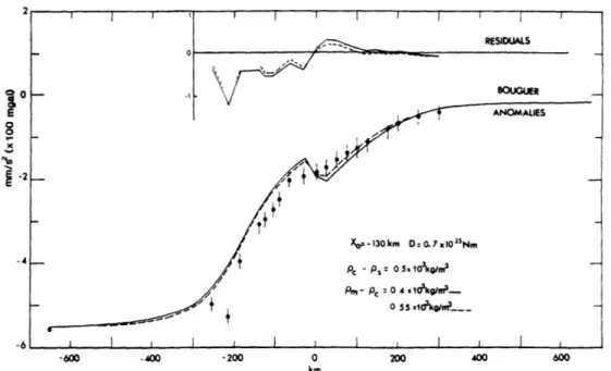
Lyon-Caen and Molnar: Gravity and Structure of the Himalaya RESIDUALS 0 o -OUGUER E ANOMALIES '2 -2 Xozz-130km D:0.7x10"Nm ~~ P, - P,: 0 5. 10kg/m 3 pm -Pe : 0 4 x1dkg/nj--0 5 5 z10kgmt -6 1 i l i l 1 1 1 1 1 -600 -400 -200 0 200 400 600 km

Fig. 6. Comparison of calculated and measured Bouguer anomalies for two different

values of the density contrast between the mantle and the crust (pm-Oc)* The density contrast between the crust and the sediments is kept constant and equal to 0.5 x 103

kg/m3. Layout as in Figure 3.

correspondingly reduced from 1.05 to 0.95 and 0.9

x 103 kg/m , calculated gravity anomalies in the

Ganga Basin differ by a maximum of only 0.10 mm/s2

(10 mGal) among the models with different density

contrasts (Figure 6) . Thus, although the density

contrast between the mantle and crust affects the shape of the plate by depressing it about 10% more

when Pm-Pc is 9.45 x 103 kg/m and 20% more wheg

0.4 x 103 kg/m than when it is 0.55 x 103 kg/m

it has almost no effect on the calculations of gravity anomalies. In our following calculations

we will keep pm~pc - 0.55 x 103 kg/m3, but even if

Pm-c is actually closer from 0.4 than from 0.55 x 103 kg/m, this would not change our conclusions

much.

Effects of the density contrast between the

crust and the sediments (Figure 7). If the density

contrast between the crust anq the sediments is

decreased from 0.5 x 103 kg/m , as assumed in mqst

of the previous calculations, to 0.3 x 103 kg/m

and if the density contrast between mantle and crust is kept constant, the plate is depressed

-600 -400 -200 0 200 400 600

Fig. 7. Comparison of calculated and measured Bouguer anomalies for different values of the density contrast between the crust and the sediments. The density contrast

between the mantle and the crust is kept constant and equal to 0.55 x 103 kg/m3. Layout

Lyon-Caen and Molnar: Gravity and Structure of the Himalaya

( a )

8

x

(cO

8

Fig. 8. Comparison of different topographic profiles and their effects. (a) L1(x) is

mean elevation within 100 km and L₂(x) within 20 km of either side of the the gravity profile; L3(x) is Bird's [19781 average elevation over the entire width of the range. Comparison of calculated Bouguer anomalies for the different loads for D - 0.7 x 1025

N m and (b) for X - -200 km and (c) for Y. - -130 km.

X₀= -200 km D= 0 7x025Nm 3 3 Pm-Pc:055x LOkg/m - c-Ps=05x 1kg/r L,x -- Ljx-- L 4x, -I I lmw -- 1 | I

Lyon-Caen and Molnar: Gravity and Structure of the Himalaya

more by only about 3%. Therefore, contrary to the density contrast between the mantle and the crust,

the density contrast between the crust and the sediments has almost no effect on the shape of the plate but increases the gravity anomalies in the

Ganga Basin by a maximum of about 0.25 mm/s2

(25

mGal) at its deepest point. This is the reason why we cannot differentiate between the two

profiles₂§0 - -125 km and Xo - -130 km with D

-0.7 x 10 N m (Figure 7).

Sensitivity of the model to the choice of the

load (Figure 8). Previous computations were

performed using a load LI(x) obtained from mean elevation along a profile 200 km wide in the region

where measurements were made (Figure 8a). The mean elevation reaches a maximum of about 6500 m at the

abscissa of the Mount Everest. For comparison we

also made computations with a load L2(x), obtained

from mean elevations along a profile 40 km wide

(Figure 8a), and a load L3(x) obtained from Bird's

[19781 average elevation over the entire width of

the range (Figure 8a). Elevations corresponding to

L2(x) are higher than for LI(x) over the Greater

Himalaya, but the maximum (~8000 m) is reached at the same abscissa. At the same time, mean

elevations over the Lesser Himalaya are a little smaller than for LI(x). The profile corresponding

to L3(x) is lower than LI(x) and L2(x) by about 2

and 3.5 km, respectively, over the Greater Himalaya and does not have a maximum elevation near the abscissa corresponding to the Mount Everest. This profile consists of an average elevation over various parts of the range that do not necessarily share the same tectonic evolution; therefore it is probably not the appropriate load to use in this study, but it provides an extreme with which to examine the uncertainities in the parameters that results from uncertainities in the load.

The differences among computed gravity

anomalies for these three profiles can reach 0.50 mm/s2 (50 mGal) for the case where the plate is

assumed to underthrust the Greater Himalaya (i.e.,

Xo - -200 km) (Figure 8b). For all these loads,

however, a plate with a constant flexural rigidity cannot underthrust the entire mountain range

(Figure 8b). Differences among calculated

anomalies are smaller for plates that underthrust

only a fraction of the range (i.e., X0 - -130 km)

(Figure 8c), and consequently, the uncertainity in the load increases the uncertainity in Xo noted

above. For instance, using Bird's (1978J profile,

the data will be best fitted with Ko - -140 km

instead of Xo - -130 km using L₂(x) (Figure 8c) or

Xo - -125 km using LI(x) (Figure 3). We present the following computations using only Lj(x), but as we have shown here, using either a larger or a smaller load will only introduce small

quantitative changes in our results.

Effect of a bending moment applied to the end of the plate. Below, we show that if a bending

moment is applied at the end of the plate that

underthrusts the entire range, the gravity anomalies cannot be fit well unless the flexural rigidity of the portion of the plate beneath the Greater Himalaya is considerably smaller than that beneath the Lesser Himalaya (Figure 13).

Summary. These calculations show clearly that a plate of constant flexural rigidity cannot

underthrust even southernmost Tibet. Models that call for wholesale underthrusting of Tibet by the

Indian shield [e.g., Argand, 1924; Powell and

Conaghan, 1973] must do so only by allowing the Indian shield to lose a considerable amount of its strength approximately 120-140 km from the front

of the Himalaya.

The calculations show that the flexural rigidity of the plate and the position of the end of the plate are constrained independently from one another. We conclude that the end of the elastic plate is between 120 and 140 km north of the

Himalayan front anj_{5that a flexural rigidity of}

about 0.7±0.5 x 10 N m, corresponding to an

elastic thickness of about 80+30 km, is necessary to explain the topographic features and the gravity field of the Ganga Basin. The fit north of the Ganga Basin, however, can be improved.

The dip of the Moho beneath the Greater Himalaya. The calculated anomalies over the Greater Himalaya and Tibet may be altered by arbitrarily changing the configuration of the Moho between the end of the elastic plate, X0, and the southern margin of Tibet where isostatic

equilibrium is assumed to prevail. If the crustal thickness of Tibet is reached 200 km from the foot of the range instead of 250 km, as assumed in Figures 3 to 8, the calculated and observed anomalies agree well (Figure 9). This corresponds to a dip of the Moho of about 15* beneath the

Greater Himalaya (provided that p-pc - 0.55 x 103

kg/m3), compared with only about 3* beneath the

Lesser Himalaya.

Possibility of subducted sediments beneath the Lesser Himalaya. In the Lesser Himalaya,

calculated anomalies are consistently 0.25 to 0.50

mm/s2 less negative than observed (Figures 5, 6,

and 7). To eliminate this difference requires the

introduction of material with low density beneath the Lesser Himalaya. The introduction of a thin

wedgj of material with a density p - 2.5 x 103

kg/m beneath the Lesser Himalaya is adequate to eliminate this negative residual (Figure 9) and suggests that sediments were probably subducted

along' with the underthrust plate.

Plate with a reduced flexural rigidity beneath the Greater Himalaya. The steeper dip of the Moho

beneath the Greater Himalaya suggests that the plate is flexed more and therefore that the

flexural rigidity is less than beneath the Lesser

Himalaya and farther south. To analyze

quantitatively this change in dip, we studied the

flexure of a plate consisting of two segments with

different flexural rigidities (Figure 2). There are now two additional parameters that we can

vary: the flexural rigidity of the northern

segment D' and the position of the junction between the two segments, now defined by X0.

First, we fix the end of the elastic plate, X',

equal to -200 km in order to mimic the structure

used in Figure 8. We seek values of D' and XO

that will lead to a plate with a shape close to that used in the computation of Figure 9. We

already know that X0 is between about -100 and

-150 km. Although the purpose of adding another

segment of plate is to fit the steepening of the

Moho beneath the Greater Himalaya, the addition of

this segment has a second important effect. The

load of the Greater Himalaya on this additional segment must be supported by the elastic strength

of the plate, and consequently, the plate is flexed down more than for the cases considered

above that ignored the support of this mass. Even

Lyon-Caen and Molnar: Gravity and Structure of the Himalaya RESIDUALS - ouSOUGUER --6 1 1 1 1 1 1 1 I I 1 1 -600 -400 -200 0 200 400 600 km

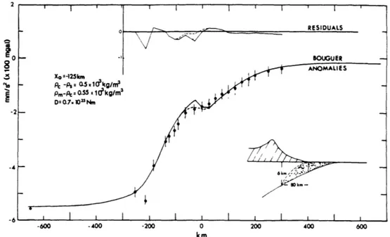
Fig. 9. Comparison of calculated and measured Bouguer anomalies. Layout as in Figure

3. Solid line shows calculated anomalies as in Figures 3-7 but with the Moho set at a

depth of 60 km at x - -200 km not -250 km, as in Figures 3-8. Note the better fit

of calculated to observed anomalies for x <-100 km than in Figures 3-8. Dashed

curve shows the effect of including a thin wedge of light material p - 2.5 x 103 kg/m3

(sediments) beneath the Lesser Himalaya. (See inset in lower right.)

a great deal, the effect of this additional load

is important. For a wide range of fJgxural

rigidities of this segment (0.2 x 10 to 0.4 x

10 N m), and Xo - -130 km or -100 km, the plate

is depressed about 50% more (Figure 10a) than for the case in Figure 9. The same effect is observed

for other values of X0 between -100 and -150 km.

The corresponding gravity profiles (Figure 10b) show that it is not possible to match the gravity anomalies by just considering a plate with a

variable flexural rigidity2 2 If XO is -19 km,

values of D' from 0.2 x 10 to 0.4 x 10 N m

allow the entire plate to be depressed too much, leading to an overall positive residual. If X is only -100 km, the entire plate is less depressed than in the case where X. is -149 km, especially

if D' is small (0.5 to 0.2 x 10 N m), but in

this case the northern segment of the plate steepens too rapidly (Figure 10).

Profiles computed using other loads (L2(x) or

L3(x)) show the same qualitative features, but the

deflection of the plate is smaller when L3(x) is

used and larger when L2(x) is used. For instance

for profiles computed with L3(x) and with Xo

--130 km, ' - -200 km, D - 0.7 x 1025 N m and D'

= 0.2 x 102 N m, the maximum depth of the basin

at x - 0 km is only 5.2 km, compared with 6.5 km

when L2(x) is used and 6.0 km when L1(x) is used

(Figure 10).

The calculations discussed in the previous section implied that an elastic plate flexed by the load of the Lesser Himalaya could account for the gravity anomalies over that region and the Ganga Basin. The results of these calculations, however, show that if the load includes the Greater Himalaya, this additional load depresses the plate too much to allow a match of calculated and observed gravity anomalies. Either additional sources or deficits of mass are required or

additional forces must operate on the plate. Inclusion of a bending moment. Rather than

appeal to additional and somewhat arbitrarily chosen excesses or deficiencies in mass, we examine the effects of other likely forces. We first investigate the effect of a bending moment applied at the end of the elastic plate. The moment both depresses the northern end of the plate and, in

reaction, elevates a portion farther south. A sufficiently large moment can flex the plate up enough to overcome the subsidence created by the additional weight. An increase in the bending moment, however, causes the northern end of the

plate to steepen. We found that a bending moment

applied at the end of a plate with XO' - -200 km

will not allow a satisfactory fit to the dati, A

bending moment of the order of 0.5 to 1.lxlO N m

is needed to elevate the plate enough beneath the Lesser Himalaya and the Ganga Basin, but in this case the slope of the northern part becomes too

large (-25*) (Figure 11). These

glculatiggs

for values of D' between21bout 10 and 10 N m.

If D' is smaller than 10 N m, the contrast

between the two flexural rigidities becomes too large, and the interaction between the two parts of

the plate is very small. The bending moment will then bend the northern part of the plate a great deal but will have very little effect on the slope or position of the plate beneath the Lesser Higglaya. On the other hand, if D' is larger than

10 N m, the difference between the two flexural

rigidities is not sufficiently large to allow the steepening observed beneath the Greater Himalaya.

We conclude that no bending moment applied 200 km north of the Himalayan front will allow a fit of observed and calculated gravity anomalies.

The position of the northern end of the plate, where the bending moment is applied, must be

farther north. If the bending moment is applied at

X* z-125km

Pc -Ps = 0.1&kg/me

Pm-#Pe 0.55 X 1dkg/m3 D=0.7.105Nm

Lyon-Caen and Molnar: Gravity and Structure of the Himalaya

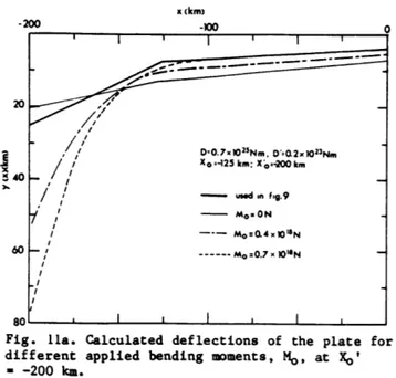
-200 X (km)

Fig. 10a. Calculated deflections of the plate for

the combination of parameters shown in Figure 10b. The heavy line shows the deflection used in Figure 9.

Xo' < -270 km, it does not change the shape of the

plate for x between -130 and -200 km enough, and if

it is applied at X0' > -230 km, it steepens the end

of the plate (-200 < x < -130) too much and too

quickly (Figure 12). Therefore if a bending moment

is applied at the end of the elastic plate, this should be between 230 and 270 km from the Himalayan front.

If the moment is applied at the end of a plate

where Xo' - -250 km, it is possible to find

different combinations of D' and of the applied

bending moment M0 that will lead to acceptable fits

of calculated and observed gravl2 y anomalies

-(Figure 13). If D' is 0.7 x 19 N m and Xo - -125

km, Mo mwgt be about 0.85 x 10 N a, but f D'

-0.2 x 10 N m, Mo need only be 0.55 x 10 N. For

the same value of D' the moment must be about 10%

larger if Xo - -150 km than if Xo - -130 km. Again

profiles comput-ed with L2(x) or L3(x) show the same

qualitative features as for L₁(x), but L2(x)

requires a larger bending moment (-0.65 x 1018 N)

and L3(x) a smaller one (- 0.45 x 1018 N) than

LI(x) (0.55 x 1018 N *).

One difficulty with applying a bending moment at x - -250 km is that although the calculated shape

of the plate is fairly close to that used in Figure

9 for x > -200 km, the curvature of the plate continues to increase beyond this point, and the

2.

I i

calculated depth of the Moho reaches 115 km at x

--250 km (Figure 11)! We do not believe that the Moho necessarily does reach such a depth. It would not be required, for instance, if we assumed that the decrease in flexural rigidity of the northern segment of the plate were accomplished by detaching the crust from the rest of the Indian lithosphere. In any case, the calculated gravity profiles

obtained directly from the flexed plate with a Moho reaching 115 km and those obtained by arbitrarily assuming that the depth of the Moho does not exceed

65 km for x < -200 km differ primarily in the range

-400 < x < -200 km (Figure 14). The data that we have are inadequate to eliminate one or the other extreme. It is interesting, however, that the profile given by Tang et al. [19811 for a portion of Tibet about 200 km farther east shows a minimum

of about 0.30 mm/s2 (30 mGal) near the

Indus-Tsangpo suture, suggesting that the crust might be deeper there than farther north or south.

We conclude that to match the gravity anomalies with an elastic plate loaded by the weight of the overthrust mountains, there must be a bending moment applied to the end of the plate.

Origin of the bending moment. If a horizontal force/unit length F acts on the end of the plate that is bent down a distance yo, then provided that this force is much less than critical buckling

strength, it produces a bending moment Mo - Fyo/2

[Parsons and Molnar, 1976]. If we assume that this

force is produced by a compressive stress a, acting on a plate of thickness H and depressed an amount

yo at its end, then a - 2IN/Hyo. If yo - 30 km, H

- 50 km, and Mo - 0.55x10 N A, a - 730 MPa (7.3

kbar). Since the horizontal compressive stress needed to maintain the high elevation and thick crustal root of Tibet is only 50 to 100 MPa [e.g., Frank, 1972; Tapponnier and Molnar, 19761, it does not seem possible to invoke a compressive stress as a mechanism to create the bending moment. We do not think that a large stress of 730 MPa can exist throughout the lithosphere.

I I D.07.10"Nm X:- 200km P-Pc=055x10akg/m3 Pe-p,= 0 510 kg/rma - -- - D'= 0 2x10" Nm X0: -100 km -- D': 0 4 ,10 3 Nm Xo=-100km D'= 0 2 x102 2 Nm X, = -130 km -- 0 0 4 .10" Nm X.: -130 km -61 -600 -400 -200 0 200 400 600 km

Fig. 10b. Calculated Bouguer anomalies for the deflections shown in Figure 10a. Layout as in Figure 3.

I I i

I I I I I I