Deep learning-based approaches for depth and 6-DoF pose estimation

Deep Learning-Based Approaches for Depth and

6-DoF Pose Estimation

OFTECHNOL

by

_FEB

_{0 5 2}

Muyuan Lin

LIBRARI

B.S., Shanghai Jiao Tong University (2015)

Submitted to the Department of Mechanical Engineering

in partial fulfillment of the requirements for the degree of

Master of Science in Mechanical Engineering

at the

MASSACHUSETTS INSTITUTE OF TECHNOLOGY

INSTITUTE OGY

020

ES

:4 C)

mo

February 2020

@

Massachusetts Institute of Technology 2020. All rights reserved.

Signature redacted

A uthor ...

...

Certified by.

Certified by...

Accepted by...

Department of Mechanical Engineering

Signature redacted

January 31,

2020

... ...

Sertac Karaman

Associate Professor of Aeronautics and Astronautics

' ' r~ C

Signature

redacted

Iesis

Nicholas M. Patrikalakis

Kawasaki Professor of Engineering

Professor of Mechaq4

Qean Engineering

Signature

redactedy "eader

Nicklas G. Hadjiaonstantinou

Professor of Mechanical Engineering

Chairman, Department Committee on Graduate Theses

MITLibraries

77 Massachusetts Avenue

Cambridge. MA 02139

http//'ibraries.mitedu/ask

DISCLAIMER NOTICE

Due to the condition of the original material, there are unavoidable flaws in this reproduction. We have made every effort possible to

provide you with the best copy available. Thank you.

The images contained In this document are of the best quality available.

Deep Learning-Based Approaches for Depth and 6-DoF Pose

Estimation

by

Muyuan Lin

Submitted to the Department of Mechanical Engineering on January 31, 2020, in partial fulfillment of the

requirements for the degree of

Master of Science in Mechanical Engineering

Abstract

In this thesis, we investigated two important geometric vision problems, namely, depth estimation from a single RGB image, and 6-DoF object pose estimation from a partial point cloud. Geometric vision problems are concerned with extracting in-formation (e.g. depth, agent trajectory, 3D structure, 6-DoF pose of objects) of the scene from noisy sensor data (e.g. RGB images, LiDAR) by exploiting geometric constraints (e.g. epipolar constraint, rigid motion of objects). Deep learning frame-work has achieved impressive progress in many computer vision tasks such as image recognition and segmentation. However, applying deep learning-based approaches to geometric vision problems, which are particularly important in safety-critical robotics applications, remains an open problem. The main challenge lies in the fact that it is not straightforward to incorporate geometric constraints, arising from image for-mation process and physical properties, to optimization problems. To this end, we explore possibilities of enforcing such constraints either by decomposing a problem into two sub-problems each respecting desired constraints, or designing an estimator establishing relationship between intermediate representations and predicted outputs. We propose a deep learning-based approach for -each problem. Through extensive ex-periments, we show that our proposed approaches produce results comparable with state of the art on public datasets.

Thesis Supervisor: Sertac Karaman

Title: Associate Professor of Aeronautics and Astronautics

Thesis Reader: Nicholas M. Patrikalakis Title: Kawasaki Professor of Engineering

Acknowledgments

I wish to acknowledge the continuous support from my thesis advisor, Prof. S. Kara-man. I would like to express my sincere gratitude for your'patience, motivation, and immense knowledge. Your guidance helped me in all the time of research and writing of this thesis. I still feel lucky to have the opportunity to have worked with you.

I would like to thank my thesis reader, also my research advisor before I join

current lab, Prof. N. M. Patrikalakis, for his insightful comments and encouragement. Thank you for your kind help throughout my preparation of qualification exams and constant support for my study and research.

Furthermore, I would like to thank the collaborators, Fangchang Ma and Varun Murali, for lending me their expertise and intuition to my understanding of research problems. I would also like to thank my fellow lab-mates Audren Cloitre, Joao Seixas de Medeiros, and many others, for all the help to further my research. The stimulating discussions with you help to widen my horizon and deepen my thinking of related research. It was a great pleasure working with you.

Last but not least, I would like to thank my family: my mom, my wife, and my sisters for supporting me spiritually throughout writing this thesis and my life in general.

The technical work presented in this thesis was funded in part by the Office of Naval Research (ONR) and Ferrovial, S.A. An earlier part of my studies and re-search were funded by the National Rere-search Foundation (NRF), Prime Minister's Office, Singapore under its Campus for Research Excellence and Technological Enter-prise (CREATE) programme. The Center for Environmental Sensing and Modeling

(CENSAM) has been an interdisciplinary research group (IRG) of the Singapore MIT

Alliance for Research and Technology (SMART) centre. Their support is greatly ap-preciated.

Contents

1 Introduction 1.1 Motivation . . . . 1.2 Overview . . . . 1.2.1 Geometric Computer 1.2.2 Deep Learning-Based 1.3 Contributions . . . . 1.4 Thesis Scope . . . .

2 Monocular Depth Estimation fr

2.1 Introduction . . . .. . 2.2 Related Work . . . . 2.3 Fakestereo-Net . . . . 2.3.1 Background . . . . 2.3.2 Network Architecture . 2.3.3 Training Loss . . . . 2.4 Experimental Evaluation . . . . 2.4.1 Datasets . . . . 2.4.2 Implementation Details . 2.4.3 Error Metrics . . . . 2.5 Results . . . . 2.5.1 Benchmark Performance 2.5.2 Performance of Stereo M 2.5.3 Results of Fine-tuning . Vision . . . Approaches

om Synthesized Stereo Pair

. . . . . . . . . . . . . . . . . . . . atching Network 15 15 17 17 20 23 24 25 25 28 31 31 32 35 37 37 37 38 39 39 40 41

2.5.4 Discussion

2.6 Conclusions . . . . 3 6-DoF Pose Estimation of Rigid Objects

3 1 Intrordiictin 3.2 Relate 3.3 Proble 3.4 Metho 3.4.1 3.4.2 3.4.3 3.4.4 3.5 Experi 3.5.1 3.5.2 3.5.3 3.5.4 3.6 Results 3.6.1 3.6.2 3.6.3 3.6.4 . 3.7 Conclusions 4 Conclusions 8 . . . . 4 2 . . . . 4 3 . . . . d W ork e. . . . . .. . . . .. . m Statement . . . . d . . . . Method Overview . . . . Segmentation . . . . 3D Geometric Features . . . .

Robust Pose Estimation . . . . m ents . . . . Implementation Details . . . . D atasets . . . . Evaluation Metrics . . . . Baselines . . . . Baseline...

Comparison with Baseline Models . . . . . Comparison with State-of-the-Art Methods

RANSAC and Least-Squares Methods . .

Running Time . . . . 45 45 48 50 50 50 52 52 53 55 55 56 57 57 58 58 59 60 61 63 65

List of Figures

1-1 Monocular depth estimation. Given an input image I (top), the task is to find a mapping <D : I - D, D is a predicted depth map of the

scene (bottom ). . . . . 18

1-2 Applications of deep learning methods in computer vision research. Im age from [50]. . . . . 21

2-1 Exemplar results. (a) Input left image (b) Ground truth right image (c) Synthesized right image (d) Predicted depth map based on real left and fake right images (e) Predicted depth map based on real left and real right images (f) Ground truth depth map from LiDAR measurement. 26

2-2 A general architecture of GANs [132]. . . . . 32 2-3 An overview of our proposed pipeline. During training, view

synthe-sis network (top) and stereo matching network (bottom) are trained independently. At inference time, the generator G takes as input an RGB image _L and predict a right view 'R of _L. The input and

pre-dicted image are fed into a stereo matching network S to estimate the corresponding depth map d of IL. . . . . 33

2-4 The architecture of cGANs. We adapt our network architectures from those in [45]. Ck denotes a convolution module with k filters. . . . . . 34

2-5 Qualitative results on KITTI depth estimation dataset. From top to bottom: input left image, real right image, predicted depth map, pre-dicted right image, ground truth LiDAR measurements. Best viewed in color. . . . . 4 1

3-1 Overview of our proposed method. The input point cloud of a target object is segmented from a whole scene using a segmentation network

[71]. A 3D ResUNet then extracts 3D geometric features from the

input point cloud. These features are used to estimate locations of each keypoint. Once keypoints are identified, the position and orientation of target objects are estimated via the singular value decomposition

(SV D ). . . . . 51

3-2 Geometric features of partial point clouds extracted by the backbone network. Features are mapped to a scalar space using t-SNE [74]. Each scan is transformed to the corresponding CAD models in black. Best viewed in color. . . . . 53 3-3 The architecture of the 3D convolutional neural network for the

predic-tion of keypoint locapredic-tion. F, K, S and D specify the number of channels of output features, the kernel size, the stride and the dilation in a 3D convolutional layer, respectively. The network takes as input a sparse tensor converted from a segmented point cloud of a target object. A

3D ResUNet is applied as a backbone network to extract geometric

features. The last layer of the network is a 3D convolutional layer with a number of output channels 312 = no x nKx nD,where nc = 13 is the

number of classes of objects in LineMOD dataset, nK= 8 the number of selected farthest points for each object, rD= 3 the dimension of each

predicted direction vector. The backbone network is adapted from [11]. Note that batch normalization is not applied after any convolutional layers in our design. . . . . 56

3-4 An example of failed predictions of keypoints. (a) an RGB image showing a target object 'ape'. (b) The ground truth direction field and the corresponding ground truth keypoint (marked as a yellow star). (c) The predicted direction field and the corresponding false prediction (marked as a red cross) of the keypoint via RANSAC. The visualized

3D direction vectors are projected onto the X-Y plane. . . . . 58

3-5 Qualitative results on LineMOD dataset. Green 3D bounding boxes

with dashed lines and blue 3D bounding boxes with solid lines represent ground truth and our predicted poses, respectively. . . . . 62

List of Tables

2.1 Performance of monocular depth estimation on KITTI depth predic-tion dataset [114]. Evaluated on the test split proposed by Eigen et

a l. [2 1]. . . . . 4 0 2.2 Performance of stereo matching algorithms. Evaluated on the test split

of KITTI dataset [114] proposed by Eigen et al. [21]. . . . . 41

2.3 Comparison of results with and without fine-tuning. . . . . 42

3.1 Comparison with baseline models on LineMOD dataset [41]. * indi-cates symmetric objects. . . . . 58 3.2 Evaluation of 6D Pose Estimation with ADD(-S) Metric on the LineMOD

dataset [41]. * indicates symmetric objects . . . . 59 3.3 Comparison between RANSAC and least-squares methods for

recov-ering keypoint locations from predicted direction fields. We report the success rates in percentage of each method on LineMOD dataset using ADD(-S) metric [41] and average runtime of RANSAC and least-squares estimators. Both methods are run on CPU without any opti-mizations. The maximum number of iterations for RANSAC is set as

Chapter 1

Introduction

1.1

Motivation

Inferring geometric cues from a scene is an important yet challenging problem in computer vision. Geometric vision is mostly about reconstructing 3D structures and estimating ego motion of cameras based on measurements from 2D images. Geomet-ric vision, especially multiple view geometry [36], has been well studied for a long history. While depth [113], optical flow or motion [43], 6-DoF pose [118] and shape analysis [70] are examples of some recent research directions. Geometric vision un-derpins various applications, such as robotic navigation [82], 3D reconstruction [46], virtual/augmented reality [25], robotic manipulation [49], object tracking [63] and scene understanding [125].

The challenges of many geometric vision problems lie in several facts. Firstly, images unavoidably lose structure information and are corrupted with noise when scenes are mapped from 3D structures to 2D images. Even worse, the same 3D point might look different at different viewpoints and under different illuminations. Secondly, the ambiguity often need to be addressed by posing additional constraints, such as spacious and temporal correlations between multiple views, and semantic reasoning, which demands higher level understanding of the scene. Last but not least, existing methods to large scale problems are often plagued by numerical challenges. Extremely large size of the input is difficult to be processed by traditional computing

infrastructures.

Deep learning is one of the most powerful machine learning frameworks for com-puter vision problems. It has achieved impressive progress on many scene under-standing problems over last decade [56, 95, 38, 106, 71]. One important advantage of deep learning-based methods is that, it is more scaleable than traditional methods which require memory proportional to the size of a scene. Deep convolutional neural networks are able to project data to concrete representations which empower deep models the capability to solve complex problems. The challenges for the design of deep neural network models lie in the difficulty of incorporating geometric constraints, generalization and robustness.

This thesis presents a study of deep learning-based methods for depth and 6-DoF object pose estimation problem. Deep learning opens up entirely new possibilities and brings exciting progress for many computer vision tasks. However, applying naive deep learning models to geometric vision problems lacks for generalization ca-pability and robustness. It greatly limits applications of learning-based approaches in real scenarios, especially in safety-critical situations. To this end, we explore pos-sibilities of explicitly incorporating geometric constraints in learning-based models. Specifically, we consider epipolar and rigid body constraint when solving monocular depth and 6-DoF pose estimation problem. Compared with end-to-end methods, our proposed approaches are able to provide better generalization capability, and achieve better performance in challenging scenarios.

1.2

Overview

1.2.1

Geometric Computer Vision

Geometric computer vision is a subclass of computer vision problems. The main goal of geometric vision is to infer 3D structures (e.g. depth, 6D pose, shape) or the ego motion of vehicles from recorded data typically with RGB and RGB-D cameras. One of the challenges of recovering 3D structures is the loss of depth information during the image formation process. In fact, the image formation process involves reflections, absorptions and interactions of lights which makes it much more complex than we might imagine. A concrete example is the depth estimation problem which is ill-posed for monocular case as there are infinite solutions given a single image input (an example of monocular depth estimation is presented in Figure 1-1). In order to accurately extract depth information, multiple view constraints are often used. However, the same 3D point in different views might look different due to illumination and occlusion. It is therefore difficult to exactly recover depth from a single image. People have been trying to infer depth from various cues like focusing

[138],

scattering [14] and shading [7]. The second challenge comes from the fact that semantic information is often desired as direct or intermediate results. For example, it is challenging to track a non-rigid object instance in a video without a high-level understanding of the object. However, semantic information cannot be directly observed and often proprietary to a human language

[52].

Image formation process is mostly described as pinhole camera model. Suppose we are trying to find a map between a 3D world point X = [X, Y, Z, 1]T (homogeneous

coordinate) and the corresponding projected 2D image point x =

[x,y,

1]T

Figure 1-1: Monocular depth estimation. Given an input image I (top), the task is to find a mapping <D : I - D, D is a predicted depth map of the scene (bottom).

terms of linear mapping of homogeneous coordinates [36]:

- -X

x

Y

where s is a scale factor, X and x are expressed in the world and camera coordinate systems, respectively. P is a 3 x 4 matrix which can be further decomposed as:

P=K[R t]

fXs

'o

K= 0

fy

vo

0 0 1

where K is the intrinsic matrix of camera.

f,

fy

are the focal length in x and y directions. no,vo are the center coordinates of the image plane. s is the axis skew modeling the shear distortion. Matrix R is a 3 x 3 rotation matrix, and column vector

t is a 3 x 1 translation vector, to represent relative transformation between world and camera coordinate frames.

There has been great progress in vision sensor technologies over the past decade. State-of-the-art robotic technologies benefit from advanced sensing capabilities such as 3D vision (e.g. stereo rigs, Time of Flights, structured light and LiDAR), wider field of view (e.g. fisheye and catadioptric lens), and event-based vision. The hardware development greatly increases the perception capabilities of robots. At the same time, it poses new challenges to the development of computational models for multiple modalities.

As aforementioned, it is often useful to take advantage of information from two or multiple views. In the setting of two cameras, image points xi andx 2 corresponding

to a common 3D world points X are related by the epipolar constraint which can be described by a 3 x 3 matrix

[36].

If cameras are not calibrated and the intrinsic matrices K are unknown, the constraint matrix is known as the fundamental matrix F and the epipolar constraint can be written as:

xfFx2 = 0

where F is a singular matrix of rank 2, i.e. det(F) = 0. On the other hand, if both cameras are calibrated and the intrinsic matrices K are obtained, the constraint matrix is known as the essential matrix E and the epipolar constraint can be written as:

x1Ex2 = 0

In addition to singularity, the two nonzero singular values of essential matrix E are identical. The fundamental matrix and the essential matrix carry all geometric in-formation. Once either the fundamental matrix or the essential matrix is estimated, the 3D structure of an observed scene can be reconstructed. For example, in a stereo rig where both camera intrinsic parameters and their relative pose (also known as extrinsic parameters) are known, 3D coordinates of observed world points can be

re-covered. If the intrinsic parameters are known but the extrinsic parameters are not, the problem is often formulated as the structure from motion (SfM) problem, or the simultaneous localization and mapping (SLAM) problem.

Based on the perspective camera model and epipolar constraint, many geometric computer vision problems, such as camera calibration, structure from motion and camera ego motion estimation, can be rigorously formulated and some are thought as solved. However, there are still open questions. For example, visual SLAM is still less accurate and robust than LiDAR based SLAM system. Feature-based visual

SLAM system tends to fail in low-texture and dynamic environments. One of the

most exciting applications for geometric vision is robotics. However, it is still lack of success in terms of long term robustness.

1.2.2

Deep Learning-Based Approaches

Deep learning is a subclass of machine learning methods that is composed of many layers of simple but non-linear modules and is fed with large amount of data to au-tomatically discover multiple levels of representations and to learn complex functions

[62]. The human pursuit of artificial intelligence has been a long history. To solve

many complex problems, such as object recognition, it is impossible to exactly define each category of objects and hand-program a recognition script to handle infinite variations of input. Deep learning allows machines to automatically extract represen-tation of the data which underlies the success of processing images and many other types of data [30]. Another powerful capability of deep learning is to automatically find the mapping from learned representation to outputs [30].

The name of "deep learning" refers to the number of layers in deep neural networks that is substantial in the context of available modern computational resources. Deeper neural network enables machines to learn features at multiple levels of abstraction and greatly boosts the representation power. Deep learning has a long history but until 2006 it was not as popular as today. The appearance of large training data, the great development of computing capability and optimization techniques all contribute to the revival of deep learning.

Semantic

Segmentation

Classification

+ Localization

Object

Detection

Instance

Segmentation

GRASS, CAT DOG, DOG, CAT DOG DOG, CAT

TREE, SKY

No objects. just pixels Single Object Multiple Object

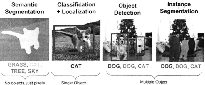
Figure 1-2: Applications of deep learning methods in computer vision research. Image from [50].

Deep learning has been deployed to many applications and achieved numerous exciting results comparing to traditional approaches (see Figure 1-2). A convolu-tional network called AlexNet [56] won the Large Scale Visual Recognition Challenge (ILSVRC) [98] and defeated traditional recognition methods for the first time. Today deep convolutional neural networks even achieve human level accuracy on the object recognition task [27]. In addition to object recognition, deep learning also achieves great success in object detection [95], neural language processing [13], recommenda-tion system [9], data generarecommenda-tion [31], just to name a few.

Why deep learning for geometric computer vision. Computer vision aims

to make computers see. To realize human level perception, it is necessary to make computers also think. Deep learning is an effective framework to learn hierarchy representations and get high level understanding of a scene. For example, corre-spondence problem, which aims to find matching pairs of image points in multiple views, is an essential building block for many geometric vision tasks (e.g. stereo depth estimation and feature-based visual odometry). Hand-crafted features is prone

to failure in low-texture areas occlusion cases. While deep neural network is able to learn representative feature automatically and aggregate global context to deal with challenging scenarios. Deep learning-based framework is the basis of the state-of-the-art matching algorithm whose performance outperforms traditional methods by a large margin[129]. In this thesis, we mainly focus on applying deep learning-based approaches to two geometric computer vision tasks: depth estimation on a single RGB image and 6-DoF pose estimation on a point cloud.

22

1.3

Contributions

To summarise, the contributions of this thesis are as follows:

" We present a novel two-stage approach for monocular depth estimation problem.

We decouple the problem into view synthesis and stereo matching problems. The view synthesis stage applies generative adversarial networks which are able to directly generate a high resolution, photo-realistic right view image. At the second stage, depth estimation is formulated as stereo matching problem in which the generated novel view and the input image compose a fake stereo pair. Our proposed method for monocular depth estimation does not need too much fine tuning therefore it is very flexible to deploy in new scenarios.

" We propose a novel geometric 6-DoF pose estimation model, termed

Geo-PoseNet, to estimate 6-DoF object pose on a partial point cloud accurately and efficiently. We adopt a 3D convolutional neural network to effectively extract geometric features and predict keypoint locations from partial point clouds.

" Our pose estimation method is robust to low resolution and self occlusion. To

show the advantage of our proposed method, we benchmark against 2D depth image regression and a PointNet-like model on LineMOD dataset [41]. Results from our method are comparable with state-of-the-art performance of RGB and RGB-D based approaches. We also release our code, to facilitate reproducibility and future research.

Chapter 2 is based on joint work with Fangchang Ma. Chapter 3 is based on joint work with Varun Murali.

1.4

Thesis Scope

The remainder of this thesis is structured as follows. We first survey and study the problem of monocular depth estimation in Chapter 2. Then we present a 3D convolutional neural network model for estimating 6-DoF object pose from noisy point cloud in Chapter 3. In each of these two chapters, we start with reviewing previous work, then present our methods in detail, and finally report experimental results on public datasets. In Chapter 4, we conclude the whole work, discuss limitations of our methods and suggest future directions.

Chapter

2

Monocular Depth Estimation from

Synthesized Stereo Pair

2.1

Introduction

Depth estimation of a scene from images is a fundamental computer vision task and has a variety of applications in scene reconstruction, 3D object recognition, localiza-tion and mapping. Most of the existing work resorts to addilocaliza-tional constraints from multiple-view geometry, such as SLAM (Simultaneous Localization and Mapping) and Structure from Motion (SfM). Unlike stereo vision or motion, depth estimation from a single image cannot use epipolar constraint and triangulation to recover ab-solute scale. Instead, monocular depth estimation takes advantage of pictorial cues, such as object size and position. Despite great challenges from the ill-posed and in-herently ambiguous problem, monocular depth estimation has recently gained lots of attentions. The single-camera setup on a platform saves payload and computational resource which is of great advantage especially in robotic applications.

The problem of depth estimation from stereo images has been extensively stud-ied for a long history. Given a pair of rectifstud-ied stereo images, the depth for each pixel can be recovered promisingly if the correspondence of the pixels between the left and right views are accurately determined. To find accurate correspondences, the main challenge comes from inherently ill-posed regions such as photometric

vari-b)

Figure 2-1: Exemplar results. (a) Input left image (b) Ground truth right image (c) Synthesized right image (d) Predicted depth map based on real left and fake right images (e) Predicted depth map based on real left and real right images (f) Ground truth depth map from LiDAR measurement.

ations, texture-less regions and occlusions. State-of-the-art stereo depth estimation algorithms usually utilize both local appearance consistency and global context infor-mation to find correspondences in ill-posed regions. Benefiting from the great power of deep convolutional neural networks, modern stereo estimation pipelines achieve much higher accuracy and speed than traditional methods.

Unlike depth estimation from stereo pairs, monocular depth estimation remains a challenging problem. In order to recover accurate depth prediction, not only various cues such as geometric information, haze, shading and texture, but also semantic understanding of the scene is necessary for posing additional constraints. As the computational capability increases continually, supervised learning on huge labeled data is possible and gradually becomes the standard pipeline of many computer vision tasks including monocular depth estimation. Supervised learning based methods of monocular depth estimation often adopt a neural network to train end-to-end and directly regress on the depth values. Though proven to be effective in improving the prediction accuracy, supervised learning consumes lots of labeled data, such as dense LiDAR measurements which are often expensive and time consuming to acquire. In addition, directly relating a single input image to the depth map without explicit geometric constraints results in the lack of generalization ability of these models.

To alleviate the use of ground truth depth data, many unsupervised learning methods have been proposed. Most of these methods [26, 28] directly regress on the disparity or depth values, and apply a spatial transformation network (STN) [47] to sample from the original input image. Upon obtaining the warped image, the input image is used as supervised signal to guide the training of depth regression. Since the disparity values are not directly compared against ground truth values, as an intermediate output, they need to be regularized by smooth constraints and left-right disparity consistency. The weights of these constraints need to be carefully tuned in order to make the training converge.

In this work, we propose an algorithm to directly predict the right view of input image, and estimate the depth map from the constructed stereo pair. Comparing to existing works, especially [73] which proposes similar two-step framework as ours, we don't explicitly predict disparity map in the view synthesis network thus avoid ambiguity in the first place. In addition, we found that simply using Li loss is not sufficient to recover fine details in images. In light of great success of generative adver-sarial networks in a variety of computer vision applications, we apply an adveradver-sarial loss in addition to an Li loss to further improve the quality of generated images. An example depth map prediction from our algorithm is shown in Figure 2-1.

Our main contributions are summarized below:

* We present a novel view synthesis approach based on generative adversarial networks which generate a high resolution, photo-realistic right view image of the RGB input. The generated novel view and the corresponding input image compose a fake stereo pair.

" Thanks to the high quality of generated novel right views, our method does not

need too much fine tuning. The generative model can be directly concatenated with existing stereo depth estimation pipelines. This makes our method very flexible to deploy in new scenarios.

" Through extensive experiments, we show that our proposed approach achieves

2.2

Related Work

In this section, we briefly overview most related work on single image depth estima-tion, stereo depth estimaestima-tion, and view synthesis.

Single image depth estimation Estimating the depth map of a scene given only

a single RGB image has been studied extensively in the literature. Prior to the emerging of deep convolutional networks, people have been trying to extract hand crafted features from various cues like focusing [138], scattering [14] and shading [7] in order to recover 3D shapes of a scene, which are known as Shape-from-X approaches. These approaches rely on some assumptions on the structure of scenes.

Saxena et al. [101] use a Markov Random Field (MRF) to incorporate global image features. Eigen et al. [21] for the first time directly train a two-stage deep convolutional network to regress the depth. They use AlexNet to get a coarse-scale prediction and then refine it locally. The work is later extended to estimate depth, normals, and semantic labels with deeper networks [20, 14]. Instead of using multi-scale training, Laina et al.

[60]

employ a single scale but deeper fully convolutional residual network [38]. While most recent researches model the depth prediction as regression problem, Fu et al. [24] propose using an ordinary regression loss to deal with the slow convergence problem of direct regression on depth.

One issue of deep neural network approaches is the requirement of a great amount of training data which might not be trivial to obtain. To address this problem,

[35, 135] utilize the synthetic image data to train a disparity prediction network

followed by a monocular depth prediction network. Ma et al.

[75]

convert sparse RGB-D depth measurements to dense map. Li et al. [68] collect Internet videos of people imitating mannequins and use multi-view geometry to acquire ground truth labeling.

Another branch of research applies unsupervised or semi-supervised learning in order to alleviate the need to use large amounts of labeled data. Garg et al. [26] formulate the monocular depth estimation as an image formation problem and and predict the depth map using a convolutional auto-encoder. Godard et al. [28] propose

28

to generate disparity images by using a cycle consistency loss and training on the stereo pairs. Kuznietsov et al. [59] use sparse ground-truth depth and stereo images to train the networks in a semi-supervised fashion. Zhou et al. [137] and Wang

et al. [115] estimate camera pose over a sequence of frames and use motion cue

as supervised signal of depth estimation task. There are also work looking at the collaboration of monocular and stereo vision. Saxena et al. [102] extract monocular cues from a Markov Random Field and incorporate them into a stereo system to enhance depth estimation performance. Luo et al. [73] propose a right view synthesis procedure followed by stereo matching of input left and generated right images.

Learned stereo Prior work of stereo depth estimation typically use hand defined similarity measures to find correspondences in stereo image pair. Some machine learning approaches apply probabilistic graphical models that learns the matching cost from the stereo images [55, 133, 103, 67]. Recent studies leverage the power of deep convolutional neural networks to obtain learned patch embeddings, and ag-gregate the matching cost by semi-global matching or Markov random field (MRF)

[126, 128, 129, 8]. They train the neural networks on large stereo image datasets and

learn visual dissimilarity between image patches. Ilg et al. [44] and Mayer et al. [78]

train neural networks end-to-end without post-processing and achieving impressive results. Pang et al.[84] propose a cascade CNN architecture to learn the disparity. Chang et al.[5] use a spatial pyramid pooling module to aggregate information from different scales.

View synthesis Works on view synthesis, i.e. generating novel views of a scene from one or multiple views, are also closely relevant to our proposed method. Given a limited number of views, recovery a novel view is underdetermined and thus re-quires incorporation of priors on the scene. Previous work relies on assumptions such as known 3D object model [94] and Lambertian reflectance [64]. Geometry-based methods aim to recover 3D structure of the scene and synthesize novel view based on the target camera pose. Garg et al. [26] and Xie et al. [119] predict disparity map

and use it to reconstruct the right view of input image. Generative models, such as generative adversarial networks (GANs) [31], variational autoencoders (VAEs)

[17], autoregressive models such as PixelRNN [83], directly predict the appearance of

target scene.

Closest to our algorithm is the work of Luo et al. [73] which also proposes a two-stage pipeline to generate a right view of the input image and estimate disparity map from constructed stereo pair. However, their view synthesis module uses the Deep3D model [119] which generates a large number of candidate values of disparity. This leads to huge memory overhead. In addition, the right hand side of the synthesized image is occluded due to a different viewpoint. Geometry-based methods like Deep3D

[119] are not able to complete the whole scene in the right view. To this end, we

apply generative adversarial networks to synthesize the right view without estimating disparity explicitly. The discriminator in the model is used to distinguish between ground truth and synthesized right view. It acts like a loss function to guide the generator to provide better estimation of the distribution of generated images. Our view synthesis module is able to generate novel views even parts of the scene are not visible in input images.

30

2.3

Fakestereo-Net

Our approach aims to decouple the original ill-posed depth estimation problem into two component stacks: a view synthesis task and a stereo matching task. The moti-vation is based on the obsermoti-vation that the information embedded in a pair of stereo images must be richer than that in a single image. Therefore, the accuracy of depth estimation from stereo matching is the upper limit of the accuracy obtained from monocular depth estimation. As the stereo matching problem is much better investi-gated than monocular depth estimation problem, we should expect a significant gain in performance of the monocular depth task if we could accurately recover the right view of the input image.

We will begin by introducing background on generative adversarial networks (GANs) [31]; then we present the network architecture of our model; and finally specify loss functions we used for network training.

2.3.1

Background

The adversarial nets framework is proposed to overcome the difficulty of approxi-mating intractable probabilistic distribution of data in the generative context

[31].

GANs consist of two networks competing with each other during training: a genera-tor G(z; 0,), where z represents a noise input variable and 0, parameters of G; and a discriminator D(x). At training time, we optimize the parameters of G and D sequen-tially: G is trained to generate samples which would ideally be consistent with the distribution of real data x, so that it can fool the discriminator; and D is trained to maximize the probability of distinguishing generated samples from real data x. The process can be described by a two-player minmax game with value function V(G, D)

[31]:

min max V(D, G) = Ex~rpa()[log D(x)] + Ez-p2 (z)[log(1 - D(G(z)))] (2.1)

Suppose both G and D are given enough capacity, there is a unique solution where G recovers the true distribution of data, and D always outputs 1/2 [31]. An illustration of GANs is showed in Figure 2-2.

Is real or fake

Discrimiator

Fake G(z) Real x

Generator

Noise

z

Figure 2-2: A general architecture of GANs [132].

2.3.2 Network Architecture

The overall pipeline of proposed method is presented in Figure 2-3. Our Fakestereo-Net adopts the design of pix2pix GANs [45] and PSMFakestereo-Net [5] with two major compo-nents:

1. Conditional generative adversarial networks used to learn a mapping from an

input image IL, to the desired right view IR of input IL.

2. A stereo matching network used to find correspondences between IL and IR and output a disparity map d.

Photorealistic view synthesis The conditional GANs (cGANs) applied in our approach are adapted from [45]. Prior work successfully applied GANs on image inpainting [122], image translation [124] and recover 3D models of objects from im-ages [120]. Aleotti et al. [2] propose to use a generator to directly estimate dense

I L G R IR

- _{-- D}

D

WaH

L

fake

m

L

RF

L : Input left image

l : real rt image

la : predicted right image

- _{D : discriminator network}

S : stereo matching network

d:predicted depth map

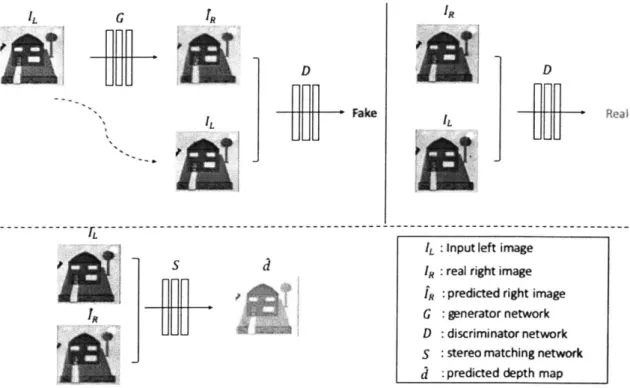
Figure 2-3: An overview of our proposed pipeline. During training, view synthesis network (top) and stereo matching network (bottom) are trained independently. At inference time, the generator G takes as input an RGB image IL and predict a right view

fR

of IL. The input and predicted image are fed into a stereo matching network

-51 C51 - ---C512 C512 1512 C256 C256 C128 C128 C64 _{Generator network C64} f~/Fake C512 C512

EC

5 12 - C256 C128 Discriminatornetwork C64

Figure 2-4: The architecture of cGANs. We adapt our network architectures from those in

[45].

Ck denotes a convolution module with k filters.

disparity map from input image, and synthesize the right view of input image using bilinear interpolation. This geometry-based method is not able to handle occlusion and regions that do not satisfy a Lambertian surface assumption. In contrast, our model directly predict the right view of input image to sidestep these limitations. Instead of using a multi-objective loss [28, 73], we apply a discriminator loss which is effective in recovering high-frequency details and does not require tuning weights of each term in a multi-objective loss. It has also been verified in our experiments that the discriminator loss helps to eliminate the blurriness and improve the realism of synthesized images.

The basic architecture of the generator is a U-Net [96] and is shown in Figure 2-4. Details of network design can be found in [45]. The network adopts an encoder structure to extract compact representation of an input image and a decoder to reconstruct an output image. The encoder only preserves high-level information due to the bottleneck structure. Since the structure of the input image is highly related to the structure of the output, it is desirable to keep low-level information in the input

image as well. To achieve this, skip connections [45] between each pair of symmetric layers in encoder and decoder are used to directly copy all channels at layer i to layer n - i, where n is the total number of layers of the generator.

Instead of supervising global context, the discriminator only penalizes structure at the scale of patches. In other words, the discriminator classifies each N x N patch in the input image is real or fake, where N is smaller than the full dimension of the input image. The discriminator is responsible for modeling high-frequency details. While low-frequency details are supervised by a Li loss as described in Section 2.3.3.

Stereo matching network We adopt PSMNet proposed in [5] for stereo matching using constructed stereo pairs. In the pipeline of PSMNet, a convolutional neural network consisting of a SPP module is used to extract features from left and right image independently. The SPP module consists of average pooling blocks of dif-ferent sizes used to discover contexts of difdif-ferent scales. Features of left and right images are then aggregated across each disparity level to form a 4D cost volume (height x width x disparity x feature size). Finally, the cost volume is fed into a series of residual blocks to predict a probability map. The predicted disparity of pixel at location (i, j) is then given by

Dmax

dijy = d xUo(-ci,j,d) (2.2)

d=O

where Dmax is a preset value of possible maximum disparity, Ci,j,d is the predicted cost for disparity d at pixel (i,j),

(-)

represents the softmax operation.

2.3.3

Training Loss

As mentioned above, adversarial loss and Li loss are used to model high-frequency and low-frequency structures, respectively. If we replaced patch discriminator with pixel discriminator, depth estimation accuracy did not change much in our experiments.

The compound objective of optimization is

G*

LcGAN(G, D)

LL1(G)

= LcGAN(GD)+ALL 1(G)

= ErLL[log D(IL, IR)] + IEr [log(1 - D(IL, G(IL)))]

SIEIL,I RI -R G(IL)11]

where A is a weight parameter for L1 loss. Note that, noise variable is not incorporated

as an input because it is found to be ignored by the network [45). For the stereo matching loss, the following objective [5] is used

L(d, d) = smoothLi(di - di), smoothL1(x) = 0.5X2 |x| - 0.5, (2-6) ifXi<1. otherwise.

where N is the number of considered pixels, d and d are the ground-truth and pre-dicted disparity, respectively.

36

(2.3)

(2.4)

(2.5)

2.4

Experimental Evaluation

In this section, we start with offering more details on datasets on which we train and evaluate our algorithm. Then we discuss implementations of our method. Finally we present evaluation metrics we applied.

2.4.1

Datasets

The KITTI depth estimation dataset We train and evaluate our algorithm on the KITTI depth prediction dataset [114]. It consists of over 93 thousand depth maps and corresponding stereo RGB images. We use the split proposed by Eigen [21] which divides the dataset into 22600 images for training, 888 images for validation, and 697 images for testing. During training, we combine training and validation sets in KITTI eigen split which consist of 23488 images in total. For the view synthesis network only the RGB images are used. For the stereo matching network, we use stereo pairs and ground truth depth maps projected from the Velodyne LiDAR measurements. To ensure results are directly comparable with previous work, during test we adopt the same crop as described in [26].

2.4.2

Implementation Details

We implement our proposed Fakestereo-Net in PyTorch framework [86] and train our model on a NVIDIA GTX 1080 Ti GPU with 11 GB memory. The full architecture of Fakestereo-Net is presented in Figure 2-3.

We train the view synthesis and stereo matching models separately. For the training of cGANs, we use Adam

[53] (1

= 0.5,

#2

= 0.999) as the optimizer with an

initial learning rate of 1 x 10-4 for the first 100 epoches. The learning rate decays linearly to zero for the second 100 epoches. For the training of stereo matching model, we also use Adam [53] (131 0.9, 02= 0.999) as the optimizer with an initial learning

rate of 1 X 10-4 and decays by half every 5 epoches. We train PSMNet for 20 epoches on the KITTI depth estimation dataset. The maximum disparity is set to 192.

Data Augmentation We augment the training data on the fly with random trans-formations:

" Crop: images are randomly cropped into size of 256 x 512.

" Color jitter: the brightness, contrast and saturation of images are each scaled by ki E [0.8, 1.2.

" Color normalization: images are normalized through mean subtraction and

di-vision by standard deviation.

" Horizontal flips: RGB images and depth maps are flipped at the same time with

a 50% chance. Notice that, when the flip is applied, the left images and right images should be swapped.

2.4.3

Error Metrics

The applied evaluation metrics, which are widely used in the literature [21], are listed below:

• 6i: percentage of predicted pixels where the relative error is within a threshold.

6i= 1/card

({y })

- card

({Qi

: max {ji/y*, y*/i} < 1.25'})

where

Di

and y* are the estimated depth and ground truth, respectively, card

(-)is

the cardinality of a set.

" Absolute relative difference: 1/card({y})Z

E{

|A - yi|/y

* Squared relative difference: 1/card({y*}) Egr ly - y*

" Root mean squared error (RMSE): 1/card({y*}) E |yII - y*||2

• Log of root mean squared error (RMSE (log)): 1/card({y*})ZET log y - log y*12

38

-2.5

Results

In this section, we present a holistic comparison between our method and others. Note that, there are different settings people apply when evaluating their proposed approaches, which easily produce different results of the same method on the same dataset. To avoid confusion, we only present results on Eigen split using raw lidar measurements as ground truth and use the widely used evaluation script from [28] to get our numbers. The official KITTI depth estimation dataset [114] provides both raw sparse depth measurements from LiDAR and post-processed ground truth depth maps. Some works use post-processed dense ground truth depth maps to evaluate their results. Evaluating on post-processed ground truth gets much better numbers even with the same method. To compare fairly with other approaches, we evaluate our method on sparse raw LiDAR measurements.

In the section below, we present and discuss results of our algorithm under different settings on KITTI depth estimation dataset.

2.5.1

Benchmark Performance

In Table 2.1, we present numeric results corresponding to depth range from 0 - 80 rn

and 0 - 50 m. Results are compared with six recent works [21, 137, 28, 59, 73, 24].

Among them, [21, 24] are supervised methods, [59, 73] and ours are semi-supervised methods, and [137, 28] are unsupervised methods.

Our proposed method achieves better results compared to [21, 137]. However, our results are worse than numbers reported in [28, 59, 73, 24]. The comparison indi-cates that our proposed method achieves reasonable performance while there is still a performance gap between state-of-the-art methods and ours. The stereo matching algorithm applied in our pipeline is a recognized state-of-the-art method. Therefore, the gap is likely because we did not perform end-to-end fine-tuning, or direct synthe-sizing of a novel view achieves sub-optimal results. Before drawing a conclusion, we present more experimental results below and come back to this question at the end of this section.

Table 2.1: Performance of monocular depth estimation on KITTI depth prediction dataset [114]. Evaluated on the test split proposed by Eigen et al. [21].

Lower is better Higher is better Approach cap Abs Rel Sqr Rel RMSE RMSEI, < 1.25 6 < 1.252 <1.253

Eigen et al. [21] 0 -80 m 0.215 1.515 7.156 0.270 0.692 0.899 0.967 Zhou et al. [137] 0 -80 m 0.183 1.595 6.709 0.270 0.734 0.902 0.959 Godard et al. [28] 0 -80 m 0.114 0.898 4.935 0.206 0.861 0.949 0.976 Kuznietsov et al. [59] 0 -80 m 0.113 0.741 4.621 0.189 0.862 0.960 0.986 Luo et al. [73] 0 -80 m 0.102 0.700 4.681 0.200 0.872 0.954 0.978 Luo et al. [73] a 0 -80 m 0.094 0.626 4.252 0.177 0.891 0.965 0.984 Fu et al. [24] (ResNet) 0 -80 rn 0.072 0.307 2.727 0.120 0.932 0.984 0.994 Ours 0 -80 m 0.141 1.057 5.20 0.233 0.810 0.932 0.972 Luo et al. [73] 0 -50 m 0.097 0.539 3.503 0.187 0.885 0.960 0.981

Luo et al. [73]a 0 -50 m 0.090 0.499 3.266 0.167 0.902 0.968 0.986

Fu et al. [24] (ResNet)b 0 - 50 m 0.071 0.268 2.271 0.116 0.936 0.985 0.995

Ours 0 -50 m 0.136 0.837 4.11 0.222 0.822 0.938 0.975

awith end-to-end fine-tuning

bwith dense depth map as ground truth

2.5.2

Performance of Stereo Matching Network

We report results of stereo depth estimation using real left and right images. We adopt the network architecture in [5] and train the model on KITTI depth prediction dataset for 20 epoches. As a comparison, we also list results from [73] in which DispFullNet [84] is applied. Luo et al. [73] train DispFullNet on the synthetic FlyingThings3D dataset [78] and fine tuned on the KITTI stereo training set [80].

Results of stereo depth estimation are provided in Table 2.2. [73] achieves better results which is likely due to larger training set is used. Nevertheless, the differences between results from two methods are not significant. Therefore, we argue that major contribution of worse results of our method reported in Table 2.1 is not from the stereo matching network.

On the other hand, accuracy of stereo depth estimation is clearly higher than that of monocular depth estimation by any reported methods 1. Since stereo depth estimation takes as input real left and right images, performance of monocular depth estimation based on two-stage pipeline, in which synthesized right view is used, cannot exceed that of stereo matching algorithms.

'Results from [24] are not considered as they are evaluated on post-processed ground truth.

40

Table 2.2: Performance of stereo matching algorithms. Evaluated on the test split of KITTI dataset [114] proposed by Eigen et al. [21].

Lower is better Higher is better

Approach cap Abs Rel Sqr Rel RMSE RMSE, J < 1.25 6T<122 < 1.25

Luo et al. [73] 0 - 80 m 0.062 0.424 3.677 0.164 0.939 0.968 0.981

Ours 0 - 80 m 0.076 0.531 3.585 0.176 0.937 0.964 0.978

Luo et al. [73] 0 - 50 m 0.058 0.316 2.675 0.152 0.947 0.971 0.983

Ours 0 - 50 m 0.074 0.423 2.862 0.168 0.940 0.966 0.980

Figure 2-5: Qualitative results on KITTI depth estimation dataset. From top to bottom: input left image, real right image, predicted depth map, predicted right image, ground truth LiDAR measurements. Best viewed in color.

2.5.3

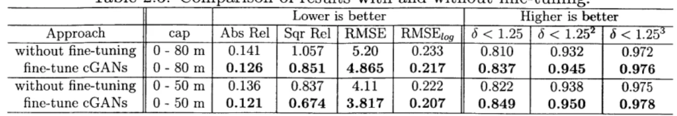
Results of Fine-tuning

We further investigate effects of fine-tuning on the performance of the two-stage pipeline. In our experiments, we fix parameters in stereo matching network, and only update parameters in the generator by computing the gradient of the loss function as described in Equation 2.6. Under these settings, we train our proposed model for 60 epoches.

Results are shown in Table 2.3. We observe significant performance gain after fine-tuning the generator end-to-end. However, the appearance of generated right view of the input image is not as realistic as that before fine-tuning. Artifacts are presented in resulting right images. The phenomenon is expected: during fine-tuning, only supervision signal of depth is used which encourages improvement of predicted structures. As a result, realistic appearance in generated images is compromised.

Table 2.3: Comparison of results with and without fine-tuning.

Lower is better Higher is better

Approach cap Abs Rel Sqr Rel RMSE RMSErog J < 1.25 J < 1.252 o__ < 1.25

without fine-tuning 0 -80 m 0.141 1.057 5.20 0.233 0.810 0.932 0.972

fine-tune cGANs 0 -80 m 0.126 0.851 4.865 0.217 0.837 0.945 0.976

without fine-tuning 0- 50m 0.136 0.837 4.11 0.222 0.822 0.938 0.975

fine-tune cGANs 0 - 50 m 0.121 0.674 3.817 0.207 0.849 0.950 0.978

2.5.4

Discussion

Considering results in Table 2.1, we can see that our initial proposed approach is able to achieve reasonable results without too much tuning and generate realistic right view of input image as shown in Figure 2-5. In general, synthesizing a novel view directly from a single image is still a hard problem. Previous works rely on strong assumptions on invariance of scene appearance among different views. Our proposed approach, in contrast, generates the right view of input image without any assumptions. From Table 2.2 and 2.3, we find that the gap between results of our approach and state-of-the-art approaches might be closed by employing a better stereo matching network, pre-training stereo matching network on other datasets, and fine-tuning the whole model end-to-end. The Li loss in fine-fine-tuning serves as a supervision signal of geometric structures of target scenes. Training the generator end-to-end while only applying an L₁ loss, however, results in artifacts in the synthesized right view.

2.6

Conclusions

In this chapter, we present a semi-supervised approach to predict the depth from a single image via decomposing the problem into a view synthesis sub-problem and a stereo matching sub-problem. Our pipeline is able to generate a photo-realistic right view of an input image. Due to the high quality of generated right images, our method does not require too much fine-tuning with the concatenated stereo network. Therefore, our method is flexible to deploy with other stereo estimation pipelines. In addition, our proposed method does not rely on strong assumptions on appearance of a novel view. Extensive experiments show that the proposed approach achieves results comparable with state-of-the-art approaches on KITTI depth prediction dataset

[114].

In future work, we would like to exploit more geometric constraints on the gen-erator in order to reduce the searching space and increase accuracy of structure es-timation. While our current method is able to effectively synthesize the fake right images regarding the geometric relationship, explicitly adding spatial transformation constraints would potentially help to speed up the convergence of training. Another interesting direction of research is to investigate how to explicitly decouple latent variables into style and structure vectors in the U-Net structure. This would greatly help us understand and control the process of view generation.

Chapter 3

6-DoF Pose Estimation of Rigid

Objects

3.1

Introduction

Real time 6-DoF (degrees of freedom) object pose estimation in clustered scene is an important yet challenging task. The success of many applications such as bin picking

[69], autonomous driving [131] and augmented reality [76] rely on accurate and robust

pose estimation. For instance, consider the problem of navigating traffic on a busy street. To estimate the likelihood of collision it is required to estimate the pose of other vehicles and possibly pedestrians on the road with reference to our vehicle. Similarly, robots operating in a warehouse are required to estimate the pose of objects in a bin to plan a successful grasp. These applications have generated a large amount of interest in this problem but existing methods tend to fail in challenging scenarios such as environments which contain small, thin, objects with limited texture.

The classical approach to 6-DoF pose estimation finds point correspondences be-tween observed target object and a corresponding CAD model in canonical view. The matching process typically relies on hand-crafted features, such as SIFT [12] for image-based methods, and FPFH [99], spin image [48] and SHOT [100] for point-cloud-based methods. However, hand-crafted features are often sensitive to noise, brittle in the presence of outliers, and can only extract local geometry.