A simple anisotropy correction procedure for acoustic wood tomography

A simple anisotropy correction procedure

for acoustic wood tomography

Hansruedi Maurer1,_{*, Sandy Isabelle Schubert}2_, Fritz Ba¨chle1_{, Sebastian Clauss}1_{, Daniel Gsell}2_, Ju¨rg Dual1_{and Peter Niemz}1

1_{ETH Zu¨rich, Institut fu¨r Geophysik, Zu¨rich, Switzerland} 2_{EMPA, Du¨bendorf, Switzerland}

*Corresponding author.

ETH Zu¨rich, Institut fu¨r Geophysik, HPP O 7, Schafmattstr. 30, 8093 Zu¨rich, Switzerland

E-mail: [email protected]

Abstract

Anisotropy of acoustic propagation velocities is a ubiq-uitous feature of wood. This needs to be considered for successful application of travel time tomography, an increasingly popular technique for non-destructive test-ing of livtest-ing trees. We have developed a simple correction scheme that removes first-order anisotropy effects. The corrected travel-time data can be inverted with isotropic inversion codes that are commercially available. Using a numerical experiment, we demonstrate the conse-quences of ignoring anisotropy effects and outline the performance of our correction scheme. The new tech-nique has been applied to two spruce samples. Subse-quent inspection of the samples revealed a good match with the tomograms.

Keywords: acoustic; anisotropy; decay; inversion

pro-cedure; tomography; trees; ultrasound.

Introduction

The stability of urban trees is an issue of increasing con-cern. Owing to the maximized utilization of space in most downtown areas, falling trees may result in significant damage to the population and/or infrastructure. It is therefore essential that fast, reliable and inexpensive testing procedures are devised to help mitigate this potential hazard. In particular, local defects caused by fungi and hidden cracks need to be detected. In situ methods using small drill holes are clearly unsuitable, since they exacerbate the decay of the trees.

Over the past few years, acoustic methods for the non-destructive testing of trees have become increasingly popular (Niemz 2001). Acoustic waves are sensitive to the elastic constants and density of wood, thus making them suitable for characterizing local defects, decay and anomalous moisture content. Standard procedures include transmission measurements along two orthogo-nal directions, in the course of which relatively low fre-quencies are used (300 Hz to 20 kHz) (Mattheck and Bethge 1992). Such procedures provide only very gross

estimates of the elastic properties and may be subject to significant systematic errors. To better exploit the infor-mation content offered by acoustic data, tomographic imaging techniques have recently been used (Socco et al. 2004). First results are encouraging, but there are several issues that need to be resolved before this tech-nique can be applied routinely.

Here, we focus on the effects of anisotropy, an impor-tant problem related to wood tomography. After a brief introduction of the inversion techniques employed, pos-sible effects of anisotropy are discussed in more detail. Then a simple correction scheme is presented that allows travel-time data recorded in tree trunks to be inverted with isotropic inversion programs that are commercially available. The benefits and limitations of our novel tech-nique are demonstrated based on synthetic data and on two authentic spruce samples.

Travel-time tomography

The general set-up of a tomographic experiment is sketched in Figure 1. Acoustic waves emitted sequen-tially from i source positions are recorded at j receiver positions. The tomographic plane, which is defined by the source and receiver positions, is subdivided into k small cells. Tomography aims to find a set of cell veloc-ities for which the computed travel times match the observed data in an optimum fashion. Usually, only the first-arriving wave trains of the recorded seismograms are analyzed. Their wavepaths can be represented by seismic rays, as indicated in Figure 1. The travel time of a seismic wave from source i to receiver j can be written as:

t sij

8

cells

where lijk is the length of the ray segment and skis the

slowness (1/velocity) of the kth cell. The relationship between the travel time and slowness can be written in matrix form:

tsGs, (2)

where vector t includes the travel times, matrix G the ray segment lengths and s the slowness values.

One of the inputs to the tomographic inversion process is an initial slowness model sini_{, with which travel times} tcalc_{can be computed. An improved slowness model s}est

that represents an attempt to minimize the differences between the calculated and observed travel times is then sought. It is common practice to minimize the squares of the differences_Ztcalc_ytobs 2_Z. An estimate of the improved slowness distribution sest_{may be found (Menke 1984) by}

568 H. Maurer et al.

Article in press - uncorrected proof

Article in press - uncorrected proof

Figure 1 Schematic diagram of the set-up for a tomographic experiment.

y

y 1

T 1 T obs calc

Dss G GqC_Ž M _. G t_Ž yt _. (3)

and substituting the result in

est ini

s ss qDs, (4)

where _C-1 is a regularization operator that may include

M

smoothing and damping constraints (Maurer et al. 1998). Formally, the tomography problem described by Eqs. (1)–(4) is linear, such that the matrix G is independent of the unknown model parameters sest_{. However, seismic}

rays obey Fermat’s principle, which requires the first-arriving wave trains to travel along the fastest path. Con-sequently, the presence of pronounced velocity contrasts may cause the seismic rays to be curved. Matrix G may thus depend on the slowness vector s. As a conse-quence, the inversion problem becomes non-linear and must be solved iteratively. After determining the initial solution of Eqs. (3) and (4), the estimated model sest_is

used as the initial model for the next iteration. This pro-cedure is repeated until the model adjustments become negligibly small.

Ray curvature also imposes problems on computation of the predicted travel times. Curved ray paths may be computed using two-point ray tracing schemes (Zelt and Smith 1992), but in the presence of strong velocity con-trasts this may lead to numerical instabilities. A more robust alternative is to compute travel times using a finite-difference approximation to the governing Eikonal equation (Schneider et al. 1992) and to reconstruct the ray paths by following the steepest descent of the result-ing travel-time fields (Aldrige and Oldenburg 1993).

Finally, we highlight a common problem in acoustic wood tomography. Owing to inherent instrumental limi-tations, it is often difficult or impossible to determine pre-cisely the difference between the origin time of the seismic pulse and the time of the first sample of the digi-tized seismogram. This time difference is generally unknown, but it usually remains constant during an

experiment. Consequently, the origin time to may be

included as a further unknown in the tomographic inver-sion procedure by modifying Eq. (1):

t sij

8

cells

As shown by Maurer (1996), it is only necessary to append a column with values of 1 to matrix G to solve the inverse problem related to Eq. (5). The solution vector

s will then include adjustments not only to the slowness

of individual cells, but also to the origin time to.

Anisotropy

A peculiarity of trees is the presence of pronounced ani-sotropy. The elastic properties and associated acoustic velocities are generally quite different in the radial, tan-gential and longitudinal directions. In tomographic exper-iments, variations of the radial and tangential velocities are of particular interest. Usually, velocities are higher in the radial than in the tangential direction.

Anisotropic wave propagation

Numerical simulations of anisotropic wave propagation are based on the equations of motion for plane strain expressed in cylindrical coordinates:

2 ≠ ur ≠srr 1 ≠srw s ysrr ww r ₂ s q q (6) ≠t ≠r r ≠w r and 2 ≠ uw ≠srw 1 ≠sww 2srw r s q q , (7) 2 ≠t ≠r r ≠w r

where urand uware displacement in the radial and

tan-gential directions ands_ij(i and j represent either r orw) are the components of the stress tensor (Gsell et al. 2004). The stiffness matrix C relates the stress tensor s and the corresponding strain tensor V (Hook’s law)

ssCV (8)

and V is related to the displacements u via a spatial operator matrix L:

VsLu. (9)

For 2D simulations in the radial-tangential plane, only three components of C are required to describe the orthotropic behavior of a tree trunk. We used a finite-difference approximation to compute the temporal and spatial derivatives in Eqs. (6) and (7), assumed stress-free boundary conditions, and modeled the excitation by presetting the stresses at specified parts of the boundary. A more detailed description of the algorithm can be found in Gsell et al. (2004).

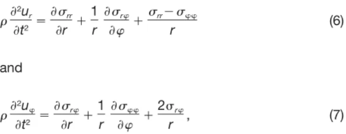
Figure 2 (a) Velocity model used for the numerical experiment. The source position is shown by the black dot. Note the anisotropy that causes the velocities to vary in the radial and tangential directions. (b) Snapshot at 245ms extracted from a finite-difference wave field simulation. (c) Travel time isochrones for the anisotropic medium as shown in (a). Solid lines represent examples of the ray paths. (d) Travel time isochrones for an isotropic medium at 1483 m s-1_{. Solid lines represent examples of seismic rays.}

Anisotropic travel time computations

The computation of travel times in anisotropic media has been extensively discussed in the literature. Some authors proposed algorithms based on ray tracing (Cer-veny 1989), while others considered finite-difference approximations to the Eikonal equation (Faria and Stoffa 1994). In this study we followed Faria and Stoffa (1994) and modified the algorithm described by Schneider et al. (1992) to yield anisotropic travel times.

Although anisotropy in its most general form is math-ematically awkward, Thomsen (1986) showed that these equations can be substantially simplified when approxi-mations for ‘‘weak anisotropy’’ are made. These approx-imations are reasonably accurate, even for materials with moderate anisotropy such as wood. For the sake of sim-plicity, we have further simplified the ‘‘weak anisotropy’’ equations and assumed elliptic anisotropy (Thomsen 1986), where the angle-dependent velocity v can be writ-ten as:

2

vsvradial_Ž1y´sin_Žfyw ,_{. .} (10)

wheref is the ray angle, w represents the azimuth of the

vradialdirection relative to the axis of the coordinate

sys-tem, and´ is the degree of anisotropy:

vradialyvtangential

´s . (11)

vradial

Numerical example

To illustrate the effects of anisotropy, we assumed a cir-cular tree trunk with a diameter of 450 mm and a realistic

ratio of the elastic constants of Cww/Crrs0.5 (Figure 2a).

Assuming a density of 546 kg m-3_{, this corresponds to}

velocities of 1483 and 1048 m s-1_{for a wave propagating}

along the radial and tangential axes, respectively. Results for the full waveform simulations are shown in the form of a snapshot in Figure 2b. The wave front advances much faster along the radial direction, resulting in sub-stantial deformation of the radiation pattern.

Results for travel-time computations using our aniso-tropic Eikonal solver are displayed in Figure 2c. For com-parison, an isotropic travel-time field using vradialis shown

in Figure 2d. As shown for the snapshot in Figure 2b, the travel-time isochrones in Figure 2c are compressed per-pendicular to the radial direction. This has important con-sequences for the geometry of the seismic rays, which are always perpendicular to the travel-time isochrones. Whereas in the isotropic case (Figure 2d) the rays are always straight, the anisotropic rays are curved, so that they travel preferably along the fast radial direction (Fig-ure 2c). Consequently, first-arriving travel times within a limited zone opposite to the source position are almost identical (;2=radius/vradial).

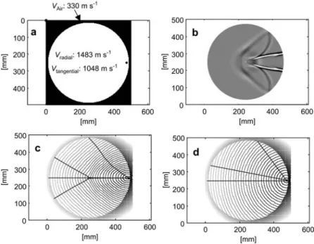
The effect of this important phenomenon is clearly evi-dent in the seismic section of Figure 3. Here, synthetic seismograms are plotted as a function of the angular dis-tance from the source. In the zone between 1108 and 2508, the onsets of the first-arriving wave trains are almost identical. For comparison, travel times obtained from our Eikonal solver are superimposed in Figure 3 (solid black line). The shape of the curves formed by the onsets in the seismograms and the computed travel times are in good agreement, thereby indicating that our simplified assumption of elliptical anisotropy is reason-able. Note that the seismogram onsets appear to be shifted relative to the computed travel times. This is

570 H. Maurer et al.

Article in press - uncorrected proof

Article in press - uncorrected proof

Figure 3 Synthetic seismic section for the set-up shown in Fig-ure 2a. Note that larger amplitudes in the seismograms were clipped to enhance the onsets of the first-arriving wave trains. The solid line depicts computed travel times with our anisotropic Eikonal solver. Dashed lines represent isotropic travel-time curves at 1483 and 1048 m s-1_{, respectively. Emergent onsets}

of the seismograms mean that the computed travel times appear to be shifted.

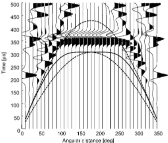
Figure 4 Tomographic results for the numerical experiment. Open dots indicate the source positions and crosses indicate the receiver positions. (a) RMS misfits for tomographic inversions using different anisotropy correction factors. The horizontal axis indi-cates tangential velocities used for computation of the correction factors. (b) Uncorrected tomogram showing radial velocities. (c) Tomogram computed with optimum correction factors associated with vtangentials1048 m s-1. (d) Overcorrected tomogram computed

with correction factors associated with vtangentials656 m s-1. Radial velocities are shown in b–d.

caused by the emergent character of the source wavelet used for the simulations. The actual onsets have small amplitudes. For comparison, isotropic travel-time curves using vradialand vtangential are also shown (dashed lines in

Figure 3). As expected from the results of Figure 2, these are inadequate representations for the travel times of waves traveling through an anisotropic medium.

Anisotropy correction factors

Ideally, the effects of anisotropy should be included in the inversion process (Pratt and Chapmann 1992). Alter-natively, by assuming that anisotropy effects of tree tomography are governed primarily by a constant radial/ tangential velocity ratio, the travel times observed can be inverted using standard isotropic travel-time tomography packages, which are widely available. For this purpose, synthetic travel times need to be calculated for a range of different anisotropy factors´. The correction factors are obtained by dividing the anisotropic travel times by the isotropic values computed using the radial propa-gation velocity. These correction factors are multiplicative and depend only on´ and the angular positions. Since they are independent of the radius, the corrections can

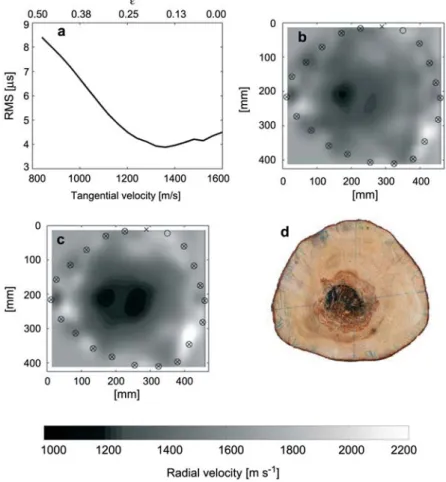
Figure 5 Tomographic results for sample A. Open dots indicate the source positions and crosses indicate the receiver positions. (a) RMS misfits for tomographic inversions using different anisotropy correction factors. The horizontal axis indicates the tangential velocities used for computation of the correction factors. (b) Uncorrected tomogram. (c) Tomogram computed with optimal correction factors associated with vtangentials1250 m s-1. (d). Photograph of sample A. The radial velocities are shown in b and c.

also be applied in cases for which the cross-section of the tree deviates from a circle.

Numerical tests with synthetic data

The effects of our correction scheme are illustrated in Figure 4. We assume the same velocity model as shown in Figure 2a and consider 36 source and receiver posi-tions equally distributed around the tomographic plane. Travel times are computed with our anisotropic finite-dif-ference Eikonal solver. Correction factors are computed for a suite of anisotropy factors´ corresponding to tan-gential velocities of 656–1483 m s-1_{. Using a value of}

1483 m s-1_{(i.e., uniform correction factors of 1) results in}

the tomogram shown in Figure 4b. The velocities are too high in the center and too low in the outer parts of the tomogram. Ignoring the effects of anisotropy resulted not only in substantial artifacts in the tomogram, but also in a relatively large root-mean-square (RMS) misfit between the computed and observed (synthetic) travel times of approximately 8ms.

We repeated the inversion procedure using all correc-tion factors and computed the resulting RMS misfits (Fig-ure 4a). As expected, application of the true tangential velocity of 1048 m s-1_{results in the smallest RMS misfit}

of 2ms. Theoretically, the misfit should be zero, but dis-cretization errors and minor numerical artifacts prevent a perfect fit between the original data and those predicted by the tomogram. The radial velocity tomogram

corre-sponding to the true correction factors associated with

v_tangentials1048 m s-1_{is shown in Figure 4c. The expected}

homogeneous velocity of 1483 m s-1_{is almost perfectly}

reconstructed, with values ranging between 1480 and 1490 m s-1_{. In contrast, overcorrecting the travel times}

with erroneously low tangential velocities of 650 m s-1

results in much larger RMS misfits of 7 ms (Figure 4a) and a flawed tomographic reconstruction (Figure 4d).

From this numerical experiment, we conclude that our correction factors are capable of accounting for first-order anisotropy effects. Furthermore, the repeated inversions required with different sets of correction fac-tors allow the average radial/tangential velocity ratio to be determined.

Applications to spruce samples

Our tomographic inversion scheme was applied to two spruce samples. Both had an average diameter of approximately 400 mm. Sample A originated from a healthy tree (Figure 5d), whereas the interior of sample B was largely decayed (Figure 6d). Data were acquired with the Fraunhofer USH system. A total of 20 source and 20 receiver positions were used for sample A, and 19 source and receiver positions were considered for sample B. In both cases, an impulsive source signal was employed and the resulting seismograms were digitized at a sam-pling rate of 0.3ms. First-break onsets were determined using an automatic picker that is based on the Akaike

572 H. Maurer et al.

Article in press - uncorrected proof

Article in press - uncorrected proof

Figure 6 Tomographic results for sample B. Open dots indicate the source positions and crosses indicate the receiver positions. (a) RMS misfits for tomographic inversions using different anisotropy correction factors. The horizontal axis indicates the tangential velocities used for computation of the correction factors. (b) Uncorrected tomogram. (c) Tomogram computed with optimal correction factors associated with vtangentials1360 m s-1. (d) Photograph of sample B. The radial velocities are shown in b and c.

information criteria (Zhang et al. 2003). This algorithm proved to be extremely reliable for our data. Most first-break onsets were determined to "2ms.

Results for sample A are displayed in Figure 5. The uncorrected tomogram in Figure 5b suggests the pres-ence of a pronounced high-velocity zone in the center of the cross-section. This is remarkably similar to the uncor-rected tomogram in Figure 4b, suggesting that this is an artifact. Consequently, repeated inversions with different anisotropy correction factors were performed. The radial velocity (1700 m s-1_{) required for our correction scheme}

was determined by averaging apparent velocities (dis-tance/travel time) computed for source-receiver pairs that were approximately opposite to each other. The curve in Figure 5a indicates that low RMS values between 3.5 and 3.75ms can be reached with tangential velocities between 1000 and 1500 m s-1_{. Figure 5c shows}

the tomogram resulting from data corrected with a tan-gential velocity of 1250 m s-1 _{(minimum of the RMS}

curve). Most of the artifacts in Figure 5b are not observed in Figure 5c. The remaining small fluctuations in the tomogram are probably minor irregularities in the wood structure of sample A that are not visible in the photo-graph of Figure 5d.

The same procedure as described for sample A was also repeated for sample B. The radial velocity was esti-mated to be ;1600 m s-1_{. For transverse velocities of}

1200–1500 m s-1_{, the RMS curve in Figure 6a shows low}

values. This indicates that the anisotropy of sample B is somewhat lower than that of sample A. The low-velocity zone shown in the tomogram in Figure 6c (computed with the optimum tangential velocity of 1360 m s-1₎

asso-ciated with the decayed region in the center of the sam-ple appears to be somewhat larger than that observed in the photograph in Figure 6d. Radial velocities within this zone vary between 1000 and 1200 m s-1_{. The decayed}

zone visible in Figure 6d is mostly air-filled, which should result in velocities of approximately 330 m s-1_(air

veloc-ity). Therefore, it must be concluded that the low-velocity zone delineated in the tomogram rather represents a region where the decay is in an intermediate state. Subtle changes in the wood color in the region surrounding the hole (Figure 6d) support this interpretation.

The fact that the decay hole is not visible in the tomo-gram as a void is an inherent limitation of travel-time tomography. According to Fermat’s principle, rays tend to avoid low-velocity zones. The resulting sparse ray cov-erage generally decreases the reliability of the tomogram in regions of decreased velocities. It is therefore often not possible to identify very low-velocity features within areas where the velocities are already decreased. Never-theless, on the basis of our tomographic reconstruction, the tree from which sample B was taken would have undoubtedly been identified as critical.

Conclusions

Conceptually, tomographic travel-time inversion is a powerful tool for non-destructive testing of trees, but ignoring the effects of anisotropy may lead to substan-tially distorted images. Our new correction scheme removes first-order anisotropy effects and leads to meaningful tomograms. This has been demonstrated with synthetic and observed data.

Together with our fully automated picking algorithm, the methodology presented is applicable with a standard laptop computer to direct field measurements. The entire sequence of picking the first breaks, determination of the anisotropy correction factors and final tomographic inversion can be performed within a few minutes. If future developments of the data acquisition procedure allow the measurements to be accomplished within a similarly short time, we suggest that acoustic tomography will become an extremely efficient tool for routinely inspect-ing urban trees.

References

Aldrige, D.F., Oldenburg, D.W. (1993) Two-dimensional inversion with finite-difference travel times. J. Seismic Explor. 2: 257–274.

Cerveny, V. (1989) Ray tracing in factorized anisotropic inho-mogeneous media. Geophys. J. Int. 99:91–100.

Faria, E.L., Stoffa, P.L. (1994) Travel time computation in trans-versely isotropic media. Geophysics 59:272–281.

Gsell, D., Leutenegger, T., Dual., J. (2004) Modeling three-dimen-sional elastic wave propagation in circular cylindrical struc-tures using a finite-difference approach. J. Acoust. Soc. Am. 116:3284–3293.

Mattheck, C., Bethge, K. Ein Impulshammer mit Laufzeitmes-sung zum Auffinden von Faulstellen in Holz. Kernforschungs-zentrum, Karlsruhe, 1992.

Maurer, H.R. (1996) Assessing systematic errors in seismic crosshole data. Geophys. Res. Lett. 23:2681–2684. Maurer, H.R., Holliger, K., Boerner, D.E. (1998) Stochastic

regu-larization: Smoothing or similitude? Geophys. Res. Lett. 25:2889–2892.

Menke, W. Geophysical Data Analysis: Discrete Inverse Theory. Academic Press, New York, 1984.

Niemz, P. (2001) Innere Defekte von Ba¨umen in Holz mit Schall bestimmt. Holz-Zentralblatt 12:169–171.

Pratt, G.R., Chapmann, C.H. (1992) Travel-time tomography in anisotropic media – II: Applications. Geophys. J. Int. 109: 20–37.

Schneider, W.A. Jr., Ranzinger, K.A., Balch, A.H., Kruse, C. (1992) A dynamic programming approach to first arrival travel time computation in media with arbitrarily distributed veloc-ities. Geophysics 57:39–50.

Socco, L.V., Sambuelli, L., Martinis, R., Comino, E., Nicolotti, G. (2004) Feasibility of ultrasonic tomography for nondestructive testing of decay on living trees. Res. Nondestruct. Eval. 15:31–54.

Thomsen, L. (1986) Weak elastic anisotropy. Geophysics 51: 1954–1966.

Zelt, C.A., Smith, R.B. (1992) Seismic travel time inversion for 2-D crustal velocity structure. Geophys. J. Int. 108:16–34. Zhang, H., Thurber, C., Rowe, C. (2003) Automatic P-wave

arri-val detection and picking with multiscale wavelet analysis for single-component recordings. Bull. Seismic Soc. Am. 93: 1904–1912.