HAL Id: tel-01926277
https://tel.archives-ouvertes.fr/tel-01926277
Submitted on 19 Nov 2018HAL is a multi-disciplinary open access archive for the deposit and dissemination of sci-entific research documents, whether they are pub-lished or not. The documents may come from teaching and research institutions in France or abroad, or from public or private research centers.
L’archive ouverte pluridisciplinaire HAL, est destinée au dépôt et à la diffusion de documents scientifiques de niveau recherche, publiés ou non, émanant des établissements d’enseignement et de recherche français ou étrangers, des laboratoires publics ou privés.
Probability distortion in clinical judgment : field study
and laboratory experiments
Marine Hainguerlot
To cite this version:
Marine Hainguerlot. Probability distortion in clinical judgment : field study and laboratory exper-iments. Economics and Finance. Université Panthéon-Sorbonne - Paris I, 2017. English. �NNT : 2017PA01E034�. �tel-01926277�
UNIVERSITE
PARIS I PANTHÉON SORBONNE
UFR
de SCIENCES ECONOMIQUES
Centre
d’Economie de la Sorbonne
THÈSE
Pour
l’obtention du titre de Docteur en Sciences Economiques
Soutenue
publiquement par
Marine
Hainguerlot
Le
21 décembre 2017
Probability
distortion in clinical judgment:
Field
study and laboratory experiments
Sous
la direction de:
Vincent
de Gardelle, Chargé de Recherche CNRSCESPSE
Jean
Christophe Vergnaud, Directeur de Recherche CNRS CES
Jury:
Ulrich
Hoffrage, Professeur à l’Université de Lausanne (Rapporteur)
Olga
Kostopoulou, Maître de Conférences à l’Imperial College of London
Pascal
Mamassian, Directeur de Recherche CNRS LSP (Rapporteur)
Jean
Marc Tallon, Directeur de Recherche CNRS PSE
Ann
Van den Bruel, Professeur Associé à l’Université d’Oxford
L’Université Paris I PanthéonSorbonne n’entend donner aucune approbation, ni improbation aux opinions émises dans cette thèse; elles doivent être considérées comme propres à leur auteur.
Remerciements
Je tiens d’abord à remercier particulièrement mes deux directeurs de thèse Jean Christophe Vergnaud et Vincent de Gardelle pour leur soutien inconditionnel durant toute la thèse. Ils ont cru en moi et m’ont donné la chance de construire ce travail durant ces quatre années. Je me considère très chanceuse d’avoir pu réaliser cette thèse à leurs côtés. Je les remercie pour leur encadrement, leur disponibilité, et nos discussions passionnées à trois. J’espère avoir la chance de pouvoir poursuivre avec eux des travaux de recherche. Ma gratitude va également aux membres de mon jury, Ulrich Hoffrage, Olga Kostopoulou, Pascal Mamassian, Jean Marc Tallon et Ann Van den Bruel, qui ont accepté d’en faire partie et qui se sont déplacés, parfois de loin. Leurs remarques et critiques m’ont été d’une aide précieuse et ont grandement contribué à l’amélioration de mon travail. Je remercie les chercheurs avec qui j’ai eu le plaisir de travailler Thibault Gajdos et Vincent Gajdos pour leur disponibilité et précieux conseils. Je remercie Thibault Gajdos de m’avoir intégré dans le groupe de travail sur la menace du stéréotype. Je remercie Vincent Gajdos de m’avoir donné l’opportunité de travailler sur les données de médecine. Je remercie aussi les chercheurs qui m’ont permis de faire mes premiers pas dans la recherche : Nicolas Soulié, Matthieu Manant, Hélène Hubert et Louis Lévy Garboua. Merci aux personnes de la Maison des Sciences Economiques (MSE) qui m’ont permis de réaliser ma thèse dans les meilleures conditions : Joël, Loïc Sorel, Jean Christophe Fouillé, Francesca Di Legge, Nathalie Louni et Leïla Sidali. Je remercie Maxim Frolov pour
l’organisation des expériences au LEEP. Je remercie Patricia Vornetti, Fabrice Le Lec et Fabrice Rossi qui m’ont confié leurs Tds pendant mes années d’ATER. Je tiens à remercier les doctorants avec qui les journées à la MSE sont toujours très heureuses: Antoine Malézieux, Feryel Bentayeb, Irène Iodice, Sandra Daudignon, Pierre Aldama, Niels Boissonnet, Antoine Hémon, Rémi Yin, Justine Jouxtel, Matthieu Cassou, Antoine Prévet, Quentin Couanau, Hector Moreno, Clément Goulet, Mathilde Poulain et Matthieu Plonquet. Un grand merci à Justine et Rémi pour avoir relu l’introduction générale. Je remercie également les anciens doctorants pour leurs précieux conseils : Noémi Berlin, Marco Gazel, Chaimaa Yassine, Anna Bernard et Sébastien Massoni. Je remercie Amalia pour sa disponibilité, son soutien et sa relecture des chapitres. Spéciale dédicace aux Cotos: Tom, Ophélie, Karl, Popo, Matoche, Quent, Tib, Bobo, Marion, Pierre, Pelletier, Nissou et Dany pour leur amitié. Merci à tous mes amis et proches : Amandine, Christophe, Jen, Amau, Shriman, Angie, Amma, Cristina, Marilou, Mathieu, Barbara, Cyrielle, Amir, Yanir, Wieder ,Jorge, Jacky, Catherine et bien d’autres. Un grand merci à la famille de Jean Christophe, Val, Loïse, Anita, Arsène, Arnold, Denise et Daniel de m’avoir accueillie de nombreuses fois pour travailler sur la thèse chez eux dans le 19ème et cet été dans le Limousin. Je remercie également le conservatoire de Maisons Alfort, en particulier Nicolas, Anton, Marie Laure, Dominique et l’orchestre, pour les fins de semaine musicales. Un grand merci à ma famille pour leur soutien, mon père Thierry, mes grands parents, Françoise et Germain, ma sœur Charlène, mon frère Simon et Aurélie. Mes derniers remerciements vont à Avshalom pour sa gentillesse et son soutien.
A ma famille.
Notice
Except the general introduction and conclusion, all chapters of this thesis are selfcontaining research articles. Consequently, each chapter contains its corresponding literature. The bibliography only contains the corresponding literature of the general introduction and conclusion.
Table
of contents
Remerciements ... 5 General Introduction ... 11 Related literature on physician versus statistical model ... 12 A theoretical framework of physician judgment ... 14 Does a biased analytical man make poorer decisions? ... 20 Combining the statistical model with the intuitive man to improve decision? ... 28 What are the factors that affect human information processing? ... 33 Part 1: Probability distortion in clinical judgment: field study ... 43 Chapter 1: Impact of probability distortion on medical decisions: a field study ... 45 Abstract ... 46 Introduction ... 47 Methods ... 49 Results ... 55 Discussion ... 63 Conclusion ... 69 References ... 69 Supplementary materials ... 73 Supplementary results ... 73 Chapter 2: Mathematics for probability distortion analysis ... 81 Abstract ... 82 Probability distortion in judgment: a single representation for different phenomena .. 83 Probability distortion in our data ... 86 Mathematical links between integration of evidence, probability distortion and Area under the ROC curve ... 88 References ... 99 Chapter 3: Statistical aids to improve medical decision accuracy ... 101 Abstract ... 102 Introduction ... 103 Methods ... 106 Results ... 114 Discussion ... 123 Conclusion ... 125 ... 126Supplementary materials ... 129 Supplementary results ... 129 Part 2: Sources of probability distortion: laboratory experiments ... 137 Chapter 4: Metacognitive ability predicts learning cue stimulus association in the absence of external feedback ... 139 Abstract ... 140 Introduction ... 141 Methods ... 144 Results ... 149 Discussion ... 155 References ... 159 Supplementary Material ... 161 Chapter 5: Perceptual overconfidence and suboptimal use of symbolic cues: A theoretical and empirical analysis ... 167 Abstract ... 168 Introduction ... 169 Methods ... 174 Results ... 176 Discussion ... 182 References ... 185 Supplementary materials ... 191 Chapter 6: Optimal probabilistic cue integration with visual evidence is limited by working memory capacity ... 195 Abstract ... 196 Introduction ... 197 Methods ... 198 Results ... 201 Discussion ... 203 References ... 205 Supplementary materials ... 209 Supplementary results ... 209 General Conclusion ... 213 Bibliography ... 219 Résumé substantiel ... 225
General
Introduction
With the advanced development of machine learning technologies, one timely question is: should we replace human judgment by predictions from the machines to improve decision making? This question is also pertinent for medical decisionmaking (Chen & Asch, 2017; Donnelly, 2017; Obermeyer & Emanuel, 2016). The purpose of this thesis is to investigate whether replacing physician judgment by statistical models can improve actual medical decision accuracy. To compare the physician with the model, we will use probability distortion as a central measure. Probability distortion corresponds to the difference between the subjective probabilities of the man and the objective probabilities of the model. This thesis shall go beyond the question of measuring how the physician performs compared to the model. This thesis also studies the cognitive processes that may drive physicians’ deviations from the model. Understanding the reasons behind probability distortion may help better address the “man versus model” debate in medical decisionmaking. In the general introduction, we develop a theoretical framework of how physicians may process information. This framework allows us to derive the cognitive mechanisms through which the physician may depart from the model, and, as a result, how his subjective probabilities may deviate from the objective probabilities. This framework will be used as a theoretical ground to motivate the questions addressed in the thesis. First, we summarize the main findings from the literature comparing physician judgment with statistical models.
Related
literature on physician versus statistical model
Prediction and Probability judgment Comparisons of predictions from statistical models with physician predictions date back to the fifties with the pioneering work of Meehl (1954). It is typically acknowledged that simple linear algorithms can better diagnose conditions or predict outcomes than physicians (Dawes et al, 1989; Grove et al, 2000; Ægisdóttir et al, 2006). However, comparisons between the probability estimates from physicians and the ones generated by statistical models have yielded mixed results on the superiority of models (for a review, see O'Hagan et al, 2006). On one hand, statistical models are found to be better calibrated: the probability estimates generated differ less from the actual frequencies. On the other hand, physicians’ probability estimates seem to better discriminate between patients who do or do not have the condition. (e.g.: McClish & Powell, 1989).
The distinct strengths of statistical models and physicians are at the core of the “man versus model” debate: how much information is available and how is the information processed? Physicians may have more information but statistical models better process the information. Statistical models’ strength: Analytical judgment Statistical models produce an analytical judgment derived from a set of assumptions specifying how to integrate the evidence. Models are known to be proficient at integrating the evidence consistently (Karelaia & Hogarth, 2008). Presented with the same set of medical evidence, statistical models may have better calibration than physicians because they optimally weight the evidence, they are not biased.
Physicians’ strength: Intuitive judgment Physician judgment involves not only analytical processes but also intuitive processes (Greenhalgh, 2002; Stolper et al, 2011; Wooley & Kostopoulou, 2013) and their intuition might be valid information (Van den Bruel, 2012). Statistical models can only generate probability estimates based on the medical evidence that they are taught to use whereas physicians may have access to more information, in particular their intuitive judgment, to better discriminate the presence or absence of the disease. Combination: statistical model + intuitive physician As a result of their complementarity, it has been recommended to capitalize on their respective strengths by combining the statistical model with the physician’s intuitive judgment to improve the accuracy of probability judgment (Blattberg & Hoch, 1990; Yaniv & Hogarth, 1993; Whitecotton et al, 1998).
A
theoretical framework of physician judgment
To address the debate “man versus model” in the thesis, we propose a theoretical framework that describes how physicians may process the information. Within this framework, we distinguish between the analytical and intuitive processes that may be involved in the physician judgment. We propose a Bayesian formalization that defines how physicians may form their clinical judgment by integrating their analytical and intuitive processes. This framework will be used as a theoretical ground to motivate the questions addressed in the thesis. A model of physician information processing During medical encounters, physicians process large amounts of information from their environment to make a diagnosis that will eventually guide their decision. Here, we adapt an informationprocessing model from Wickens et al. (2015) to the medical encounter situation. Below, we describe a simple fourstage model of physician information processing (see also Figure 1). (1) Inputs: The physician collects information about the patient (diagnosis cues) in two ways. Some cues (��) are explicit in that they take a particular value. For example, the physician observes that the temperature of the patient is 37°C. The physician may also receive an internal signal (�) which corresponds to an impression about the presence or absence of the disease and that cannot be articulated easily to the diagnosis cues. For example, the physician may have the feeling that something is wrong with the patient without being able to explicit why.
(2) Central processing: As aided by her prior knowledge and experience, she retrieves from her longterm memory a meaningful interpretation about the association between information collected in the samples and the occurrence of the disease. For example, she considers that observing a temperature of 37°C is usually reassuring. On the other hand, she remembers that her feeling that something is wrong with the patient has already been a red flag with other patients. Overall, she holds in working memory two informative components: an analytical component (i.e. the evaluation of the explicit cues) and an intuitive component (i.e. the evaluation of her internal signal). She then integrates the analytical and intuitive components together to judge whether or not the patient has the disease.
(3) Decision: The physician decides to treat or not the patient as a function of her judgment about whether or not the patient may have the disease and the consequences associated to her decision. (4) Learning: Finally, after observing the outcome of her decision the physician may update the meaningful interpretation she attributes to the information collected. She then stores the updated valuation into her long term memory. Note that these stages depend on several cognitive abilities: working memory, longterm memory, attention resources and effort. Below, we shortly describe their potential roles in the information processing model. Working memory: Working memory is essential for holding and manipulating information in the short term: “It is the temporary store that keeps information active while we are using it or until we use it.” (Wickens et al, 2004). Working memory is required to keep the analytical and intuitive components active to integrate them together. It is also
necessary to update the value of the diagnosis cues on the basis of the information arriving from the outcome (i.e. the feedback). Long term memory: Longterm memory is responsible for storing and retrieving information about the value of the diagnosis cues in the longterm. It corresponds to the process of learning. Attention resources and effort: In particular, selective attention is necessary to select which diagnosis cues to process (the ones with the highest perceived informative value) and which diagnosis cues to filter out. The ability to do several tasks at one time, to allocate the attention resources and effort to different tasks is also required.
Figure 1: A simple physician information processing model Bayesian model of central information processing
We model how a physician forms her clinical judgment about whether or not the patient has a disease: � = 1 or � = 0. First, we define the evaluation of the explicit cues and the
internal signal. Second, we model how the analytical and the intuitive components are integrated into the clinical judgment. The model is developed in log odds. For the sake of simplicity, we assume that the explicit cues �� and the internal signal � are independent.
Samples of diagnosis cues ��
The physician observes the values taken by the explicit cues (��) and the internal signal (�). For the sake of simplicity, we consider that the explicit cues can take 2 values: 1 or 0.
Knowledge about �� and �
We consider that the physician holds in her longterm memory knowledge about the sensitivity ��(�� = 1|� = 1)1 and the specificity ��(�
� = 0|� = 0) of the explicit cues ��.
Similarly, the physician stores in longterm memory the probability distribution of the internal signal conditional on the presence ��(�|� = 1) or absence of the disease ��(�|� = 0).
Evaluation of the explicit cues
According to this knowledge, she evaluates each cue �� by calculating the weight of evidence (log odds) as follows: ����=� = ln ��(��=�|�=1) ��(��=�|�=0) where � = 0,1. The analytical component corresponds to the sum of the weight of evidence of �� : ∑ ���=1 ���. Evaluation of the internal signal
We postulate that the physician also evaluates her internal signal by the weight of evidence as follows: ��=�� = �� (� �(�=�|�=1) ��(�=�|�=0)), where � ∈ ℝ ��� corresponds to the intuitive component. Integration of analytical and intuitive components Finally, she forms her subjective probability by revising her prior belief on the disease ������� (� = 1) through the following integration equation: ������(�=1|�,�)(�=0|�,�)= �� ������� (�=1) ������� (�=0)+ � ∑ ���=1 ���+ ���� (eq1) Where the parameters � and � capture how the physician may distort the analytical and intuitive components respectively. Physician versus ideal clinical judgment Overall, the physician may suffer from several biases in the way she processes and integrates the information. First, she may misevaluate both the analytical and the intuitive components with respect to their objective values ���� and ���. Second, she may inaccurately integrate the analytical and/ or intuitive component(s).
Terminology In the remaining of the thesis, we use the following terms: “Statistical model”2: judgment generated by a set of assumptions specifying how to best integrate the evidence. “Analytical man”: part of the physician’s judgment explained by an analytical integration of the evidence “Intuitive man”: part of the physician’s judgment explained by intuition Physician judgment: physician subjective probability estimate that a patient has the disease. Physician decision: physician decision to treat or not to treat. Questions addressed in the thesis Within this framework, the thesis addresses the following three questions: Does a biased analytical man make poorer decisions? Does combining the statistical model with the intuitive man improve decision? What are the factors that affect human information processing?
Does
a biased analytical man make poorer decisions?
As described previously, physician judgment involves not only an analytical component but also an intuitive component. The extent to which physicians use analytical and intuitive processes may vary. Thus, even if it is well documented that physicians are biased in their analytical integration of the evidence, it may not have an impact on the quality of their decision. For example, physicians could rely on their intuition alone to make a decision. Also, their intuitive component could offset their biased analytical component. In chapter 1, our goal is to evaluate, using medical data from the field, whether a biased analytical physician makes poorer decisions. Our set of medical data contains for each patient: information regarding the presence or absence of the disease, the available medical evidence, the physician’s probability judgment that the patient has the disease and her treatment decision. Within our theoretical framework, physician’s judgment is composed of two components: an analytical part and an intuitive part. We need to separate these two components. Operationally, we propose to separate the physician’s judgment into two components: the linear judgment and the residual judgment. We define the analytical component as a linear judgment that contains the part of the physician’s judgment that is explained by a linear integration of the medical evidence. The intuitive component corresponds to the residual judgment which captures the part of the judgment that is not explained by a linear integration. It may capture physicians’ intuition but also physicians’ ability to integrate the evidence in a nonlinear way. To assess whether the physician is biased in his linear judgment, we compare the physician probability predicted by the linear judgment to the disease probability predicted by the linear model. We quantify bias in the analytical part asthe distortion between the physician probability predicted by the linear judgment and the disease probability predicted by the linear model. Finally, we test whether probability distortion impairs the accuracy of medical decision. Method Figure 2 illustrates our method. Lens Model approach How good is the physician at integrating the available medical evidence compared to a statistical model? To answer this question, we use the Lens model approach (Brunswick, 1952; Goldberg, 1970). We consider that the physician judgment and the presence or absence of the disease being predicted can be modeled as two separate linear functions of cues available in the environment (Dawes & Corrigan, 1974; Einhorn & Hogarth, 1975). The presence or absence of the disease is modeled as a linear function of a set of cues ��, � = 1, . . , �, as follows: ������(� = 1|�)(� = 0|�) = ���+ ∑ ��� � �=1 �� (eq2a) Similarly, physician probability judgment that a patient has the disease is modeled as a linear function of a set of cues ��, � = 1, . . , �, as follows:
������(� = 1)(� = 0) = ���+ ∑ ��� � �=1 ��+ � (eq2b) where the error term � corresponds to the “residual judgment”.
Interpretation of ��� versus ���
The coefficient �� corresponds to the log odds ratio for a given cue ��. Odds define the likelihood that the disease will occur:
���� =�(� = 1)�(� = 0)
The odds ratio corresponds to the odds that the disease will occur given that �� = 1
compared to the odds that the disease will occur when �� = 0. The odds ratio measures the association between the presence or absence of the disease and the cue ��: ���� ����� = �(� = 1|�� = 1) �(� = 0|�� = 1) �(� = 1|�� = 0) �(� = 0|�� = 0) We can observe that the way the physician weights the cues in terms of log odds ratio ��� can differ in two distinct ways compared to ���. First, she can over or under weight relevant cues (over or under weighting bias): ��� ���< 1 or ��� ��� > 1. Second, she can weight irrelevant cues (misweighting bias): ��� ≠ ��� = 0. Probability distortion analysis: Linear judgment versus linear model By applying the corresponding regression weights to the cues, we can estimate in log odds (��(�) = �
1−�) the physician probability predicted by the linear judgment (��(�̂)) and the �
disease probability predicted by the linear model (��(�̂)). To compare the linear judgment � with the linear model, we plot ��(�̂) versus ��(�� ̂). �
We use the general linear model to estimate a slope parameter of the distortion when probabilities are transformed in log odds, as follows: ��(�̂) = �� 0+ �1��(�̂)� 3 (Zhang & Maloney, 2012).
When �1=1, there is no distortion in the slope. When �1 < 1, physicians overestimate small probabilities and underestimate large probabilities. When �1 > 1, physicians under
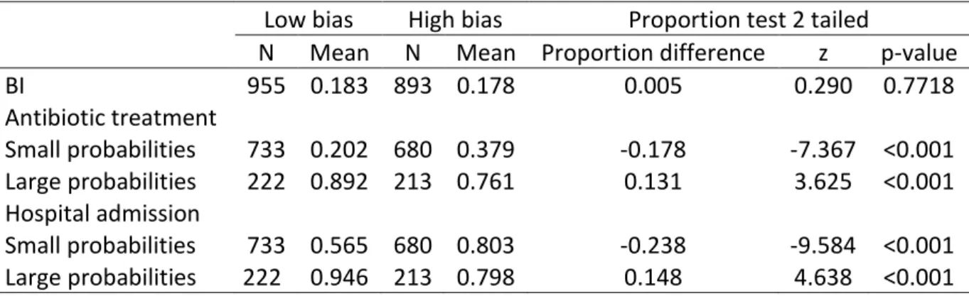
estimate small probabilities and overestimate large probabilities. Does a bias in probability distortion impair the accuracy of medical decision? Empirically, we separate the dataset into 2 groups of patients based on the physician probability judgment: a high bias and a low bias group such that in the high bias group the distortion is greater compared to the low bias group. We investigate whether the accuracy of medical decision is impaired in the high bias group compared to the low bias group. To evaluate the accuracy of medical decision, we consider two measures: the sensitivity (i.e. the proportion of patients with the disease who receive treatment) and the specificity (i.e. the proportion of patients without the disease who do not receive treatment). Data We applied our method to the detection of bacterial infection in febrile infants younger than 3 months (N=1848) and assessed its impact on two dimensions of heath care (antibiotic treatment and hospital admission). Our data come from a prospective cohort study of the procalcitonin biomarker in the detection of bacterial infection in febrile infants younger than 3 months (Milcent et al., 2016). Physicians were asked to record the information they
collected about patients from their admission to their discharge. They recorded the demographic and neonatal data, medical history, physical examination, and clinical findings from ordered laboratory tests. Physicians were required to report their probability estimate that the infant had a bacterial infection, on a scale from 0 to 100% at two stages of the data collection: (i) at the end of the physical examination (pretest probability); and (ii) after receiving the clinical findings from the laboratory tests (posttest probability). Following the second estimate, they reported their decisions to hospitalize and to treat with antibiotics.
Figure 2: Diagram of the Lens model approach applied to judgment
Remark about the relationship between the estimates �� from the Lens model approach and the theoretical biases in evaluation and integration from the Bayesian framework
Note that the comparison between the estimates from the Lens model approach i.e. ��� (in equation 2b) versus ��� (in equation 2a) allows us to study whether physicians weight the evidence in a different way compared to the objective weights. However, and as it is
described below, we cannot disentangle whether the difference in weights is related to a bias in integration and/ or a bias in evaluation of the evidence as formalized with the Bayesian framework (in equation 1). ��� and � �� In equation 2b, ��� corresponds to the difference ceteris paribus in the subjective probability (in log odds) between patients with �� = 1 and patients with �� = 0.
In equation 1, this difference is equal to �(�� �=1 � − � ���=0). Thus we have: ��� = �(�� �=1 � − � ���=0). In equation 2a, ��� is equal to �� ( ��(�=1|��=1) ��(�=0|��=1) ��(�=1|��=0) ��(�=0|��=0) ). Note that by Bayes rule: �� ( ��(�=1|��=1) ��(�=0|��=1) ��(�=1|��=0) ��(�=0|��=0) ) = �� ( ��(��=1|�=1) ��(��=1|�=0) ��(��=0|�=1) ��(��=0|�=0) ) where �� ( ��(��=1|�=1) ��(��=1|�=0) ��(��=0|�=1) ��(��=0|�=0) ) = �������������/(1−�����������)(1−�����������)/�����������= ����=1− ����=0. The ratio �����������/(1−�����������) (1−�����������)/����������� is sometimes called the diagnostic odds ratio (see Glas et al, 2003). Over/ under weighting bias (��� ���) and misweighting bias (��� ≠ ��� = 0) The over or under weighting bias ��� ��� corresponds theoretically to �(���=1� −���=0� ) ���=1� −���=0� . It can be the consequence of two biases in the analytical judgment: a bias in the knowledge of the diagnostic odds ratio: ����=1− ����=0 ≠ � ���=1− ����=0 a bias in the integration of the evidence: � ≠ 1
The misweighting bias ��� ≠ ���= 0 corresponds theoretically to �(�� �=1 � − � ���=0) ≠ ����=1− ����=0 = 0. It can be the consequence of a bias in the knowledge of the diagnostic odds ratio: �� �=1 � − � ���=0 ≠ 0.
Remark about the relationship between the estimates �� from the Lens model approach and the shape of the probability distortion
Note that the shape of the probability distortion in log odds between predicted physician’s probability judgment and the predicted disease probability depends on the value of the corresponding estimates from the Lens model approach ��� (in equation 2b) and ��� (in equation 2a) . Chapter 2 discusses the shape of the distortion as a function of the estimates βi .
Combining
the statistical model with the intuitive man to improve decision?
In the theoretical framework, we documented that physicians may suffer from several biases in the way they process and integrate the information. First, they may misevaluate both the analytical and the intuitive components with respect to their objective values �� � � and � ��. Second, they may inaccurately integrate the analytical (�) and/ or intuitive (�) component(s). How can we replace physician judgment by statistical models to improve the quality of judgment? Operationally, we can replace the analytical man (�����) by the
statistical model (��
�
�). However, we do not observe the optimal value of intuition (� ��).
Thus, the best we can do to improve physician judgment, would be to optimally combine the statistical model (����) with the intuitive man (���). The efficacy of this combined approach to improve the accuracy of judgment is well documented (Blattberg & Hoch, 1990). However, whether or not such combined statistical scores can improve the accuracy of actual decisions remains an open question. Indeed, some studies in the literature suggest that physicians’ decisions do not fully depend on their judgment (Sorum et al., 2002; Beckstead, 2017). Physicians’ decision departure from the judgment may be also relevant. In chapter 3, our goal is twofold: (1) to evaluate, using medical data from the field, whether combining the statistical model with the intuitive man can improve decision; (2) to assess, on the same dataset, whether physicians’ actual decision deviate from their expected decision, that is to say the one produced by their judgment, and if so, whether this deviation constitutes relevant information that should be accounted for when designing a combined statistical score.
Our analysis is performed on the same set of medical data, previously described in chapter 1. To measure the statistical model and the intuitive man, we use the same identification approach than the one previously described in chapter 1 (i.e. the Lens model approach). We define physician expected decision to treat as a linear integration of diagnosis cues and their judgment. Deviation from expected decision to treat is the difference between the actual decision and the expected decision. We estimate two statistical scores that combine: (1) the statistical model and the intuitive man, (2) the statistical model, the intuitive man and the observed deviation from expected decision. Finally, we test whether these two combined statistical scores can improve actual decision accuracy. Methods Statistical score combining predicted disease probability and residual judgment We estimate the combined statistical score as the best fitting model for predicting the presence or absence of the disease given the predicted disease probability in log odds (��(�̂)) and the residual judgment (�), as follows: � ���(� = 1|��(�̂), �)� �(� = 0|��(�̂), �) = �� 0 + �1��(�̂) + �� 2� Statistical score combining predicted disease probability, residual judgment and residual decision Residual decision Here, we describe our method to identify physician deviation from expected decision (“residual decision”). Figure 3 summarizes the method.
First, following the same Lens model approach as described in section 1, we model the decision to treat (�) as a linear logistic function of the cues �� and the physician probability judgment in log odds (��(��)), as follows:
���(� = 1|�, ��(��(� = 0|�, ��(���)) ))) = ���+ ∑ ��� � �=1 ��+ �����(��) By applying the regression weights, we estimate in log odds the predicted probability of treatment (��(�̂)). � Second, we measure residual decision (�), as the difference between the actual decision to treat in log odds and ��(�̂), as follows: �
{ ln ( 0.99 0.01) − ��(�̂),� �� ������ �������� �� �� ����� ln (0.010.99) − ��(�̂),� �� ������ �������� �� �� ��� ����� where we choose to attribute the value ��0.99 0.01 if actual decision is to treat and �� 0.01 0.99 if actual decision is to not treat, to handle infinite values. The residual decision contains the part of physicians’ decision that is not explained by physicians’ judgment and a linear integration of the cues. Statistical score Finally, we estimate the combined statistical score as the best fitting model for predicting the presence or absence of the disease given the predicted disease probability in log odds, the residual judgment (�) and the residual decision (�) as follows:
���(� = 1|��(�̂), �, �)� �(� = 0|��(�̂), �, �) = �� 0+ �1��(�̂) + �� 2� + �3� Can a combined statistical score improve the accuracy of medical decision? Empirically, we determine the decision threshold for each combined score that maximizes specificity (i.e. the proportion of patients without disease who do not receive treatment) under the constraint that sensitivity (i.e. the proportion of patients with disease who receive treatment) is equal to the sensitivity of the actual treatment decision. We can then compare the specificity obtained with the combined statistical score to the actual specificity. Data We apply our method to the dataset presented in the previous section.
Figure 3: Diagram of the Lens model approach applied to decision
What
are the factors that affect human information processing?
In the theoretical framework, we documented that physicians may suffer from several biases in the way they process and integrate the information. First, they may misevaluate both the analytical and the intuitive components with respect to their objective values ���� and ���. Second, they may inaccurately integrate the analytical (�) and/ or intuitive (�)
component(s).
What are the factors that affect human information processing?
In chapters 4, 5 and 6, we investigate potential sources of misevaluation of the analytical component4(chapter 4) and inaccurate integration of the analytical and intuitive
components5 ( (chapters 5 and 6). The first factor that we study is working memory. It is well documented that the ability to maintain information in working memory is limited in time and capacity (for a review, see Wickens et al, 2015). The second factor that we study is the misevaluation of the intuitive component6 as “intuition is sometimes marvelous and sometimes flawed” (Kahneman & Klein, 2009). In chapter 4, we test whether people’s ability to learn about the value of the analytical component, in the absence of external feedback, depends on the quality of their intuitive component. We reason that, in the absence of external feedback, the only source of information that may help people to learn about which diagnosis cues is relevant or not is their intuitive component. Furthermore, we test whether working memory is also necessary to learn in that situation. 4 i.e. � ��� ≠ ���� 5 i.e. ��������� (�=1) � (�=0)+ � ∑ ���=1 ��+ ����≠ �������� � (�=1) � (�=0)+ ∑ ���=1 ��+ ���
In chapter 5, we investigate whether people’ ability to integrate the analytical and intuitive components depends on the quality of their intuitive component. We consider that people may misevaluate their intuitive component, which would affect the quality of the integration process. In chapter 6, we investigate whether people’s ability to integrate the analytical and intuitive components depends on their working memory capacity, as we hypothesize that this capacity is required to manipulate information during this stage. To measure the way people value and integrate the analytical component, we consider the simple situation where only one explicit cue is available. Valuation of the explicit cue is measured by a subjective report when objective value is not available. Integration of the explicit cue is measured by observing how it is used when objective value is known. To measure the quality of the intuitive component, we propose to use confidence in one’s own decision, when no explicit cue is available to make the decision, as a measure of the value one attributes to the intuitive component. To test our hypotheses about the impact of these two factors, we ran two experiments with a simple perceptual decision task. In one experiment, participants had to learn the value of an explicit cue, in the absence of external feedback. In another experiment, participants were asked to integrate an explicit cue (whose informative value was provided to them) with the perceptual stimulus. For each experiment, we measured working memory and confidence in decision separately. Method
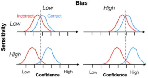
In the following section, we develop the method to measure the quality of the intuitive component and the method to measure the ability to integrate the analytical and intuitive component. Measuring the quality of the intuitive component As previously described, to measure the quality of the intuitive component, we propose to use confidence in decision. Hereafter, we describe the measures used to assess the quality of confidence ratings (Fleming & Lau, 2014). From confidence ratings, it is important to distinguish between bias and sensitivity. Bias in confidence, also called under or overconfidence, corresponds to the tendency to give low or high confidence ratings. Sensitivity in confidence corresponds to the ability to distinguish between one’s correct and incorrect responses. Figure 4, below, illustrates schematically the difference between sensitivity and bias. The blue and red distributions represent respectively the confidence ratings when the observer is correct and incorrect. For example, an observer can be good at discriminating between her correct and incorrect responses (high sensitivity) but display overconfidence overall (high bias). We quantify the accuracy of the observer’s intuitive component by measuring both dimensions: bias (overconfidence) and sensitivity (metacognitive sensitivity).
Figure 4: Schematic representation showing the difference between confidence sensitivity
and bias. From “How to measure metacognition” by Fleming, S. M., & Lau, H. C
(2014). Frontiers in human neuroscience, 8. Measuring the ability to integrate the analytical and intuitive components To assess the extent to which participants are able to integrate the analytical and intuitive components, we need an optimal benchmark. To determine how both components should be integrated ideally, we need to know the objective value of the intuitive component (i.e. the internal signal). We use Signal Detection Theory (SDT) (Green & Swets, 1966) which proposes a formalization of the internal signal. Hereafter, we present the SDT framework and our measure of integration. Signal Detection Theory Transcribed in our medical framework, the SDT model assumes that the internal signal of the observer follows a Gaussian distribution conditional on the presence of the disease (� = 1) (~�(+�′ 2⁄ ,1)) or the absence of the disease (� = 0) (~�(−�′ 2⁄ ,1)). The distance
between the two Gaussian curves is equal to �′, named sensitivity, which corresponds to the observer’s ability to discriminate between disease present or absent. The observer sets a
decision criterion � on her internal axis that determines above which level of internal signal she will answer “Y=1” (i.e. “Disease present”). Figure 5 illustrates the SDT model.
Figure 5: Diagram of SDT model Following this model, the probability of the physician response depends on criterion �, sensitivity �′ and the patient condition � as described in the table below. Patient condition Disease No disease Physician response
Say “Y=1” �(“Y = 1”|� = 1)
= 1 − �(−�′⁄2+ �) �(“Y = 1”|� = 0)= 1 − �(�′⁄2+ �) Say “Y=0” �(“Y = 0”|� = 1)
= �(−�′⁄2+ �) �(“Y = 0”|� = 0)= �(�′⁄2+ �) where �(�) = ∫ 1 √2� � �=−∞ �− 1 2�2��. SDT parameters estimates criterion � and sensitivity �′ The parameters � and �′ can be inferred from the observer’s response by computing �(“Y = 1”|� = 1) and�(“Y = 0”|� = 0), as described below.
�(“Y = 1”|� = 1) = 1 − � (−�′⁄2+ �) = � (�′⁄ − �)2 Then �′⁄ − � = �(�(“Y = 1”|� = 1)2 ) where �(�) = �−1(�)
�(“Y = 0”|� = 0) = � (�′⁄2+ �) Then �′⁄2+ � = �(�(“Y = 0”|� = 0)). Thus �′ =�(�(“Y = 1”|� = 1)) +�(�(“Y = 0”|� = 0)) � = 12 (�(�(“Y = 0”|� = 0))− �(�(“Y = 1”|� = 1)) SDT application: the observer receives one explicit cue �1 and an internal signal � Here we derive the optimal integration of the explicit cue �1 and the internal signal �. Given the cue �1, the internal signal � and the objective prior ������� (� = 1), the Bayesian observer forms her posterior belief according to Bayes rule, as follows:
������(� = 1|�(� = 0|�1, �)
1, �) = ��
������� (� = 1)
������� (� = 0) + ���1+ ���
The Bayesian observer decides to respond "� = 1" if ����(�=1|�1,�)
��(�=0|�1,�)> 0
The optimal decision criterion ����(�) is the value of � such that ����(�=1|�1,�)
��(�=0|�1,�)= 0 Within the SDT framework, we can compute the objective weight of evidence of the internal signal �, as follows: ���= �� (� �(�|� = 1) ��(�|� = 0)) where ��(�|� = 1) = 1 √2� � −12(�−�′/2)2 and ��(�|� = 0) = 1 √2� � −12(�+�′/2)2 ���= �� (�−12(�−�′/2) 2 �−12(�+�′/2)2) = ��′ Thus
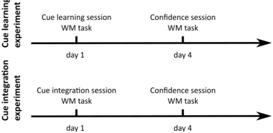
������(� = 1|�(� = 0|�1, �) 1, �) = �� ������� (� = 1) ������� (� = 0) + ���1+ ��′ The optimal decision criterion is equal to: �∗ = − 1 �′(�� ������� (� = 1) ������� (� = 0) + ���1) ≡ ���� Criterion adjustment We quantify the extent to which the observer is able to integrate the explicit cue �1 (i.e. analytical component) and the internal signal � (i.e. intuitive component) with respect to the ideal integration as the observer’s deviation from the optimal decision criterion: ���� ����. Data Experimental protocol We ran two experiments (for details about the experimental protocol, see Figure 6). In each experiment, participants engaged in a simple perceptual decision task: they had to identify which of two sets presented on the computer screen contained more dots (see Figure 7a). Each participant completed two experimental sessions, 4 days apart. The order of the two sessions was counterbalanced across participants. In the cue learning experiment (N=65), participants engaged in a “cue learning” session and a “confidence” session. In the cue integration experiment (N=69), participants engaged in a “cue integration” session and a “confidence” session. Each session started with a working memory task. The data of the cue learning experiment are analyzed in chapter 4 and the data of the cue integration experiment are analyzed in chapters 5 and 6. Below we describe each session.
Figure 6: Cue learning experiment (N=65) and cue integration experiment (N=69). The order of the two sessions was counterbalanced across participants. “Cue learning” session: Each trial started with a central cue. The cue was a square, a circle or a triangle. One shape predicted the left category, one predicted the right category (both with probability p=0.75) and one provided no information about the forthcoming category. Participants were not informed about the associations between the cues and the probabilities of occurrence of a stimulus but they were informed that there were a 'left', a 'right' and a 'neutral' cue. At the beginning of the session, they were required to learn about the cuestimulus associations, in order to optimize their decisions and they were told that at the end of the session, they had to report these associations (e.g.: Which shape was predictive of the left category?) “Cue integration” session: Each trial started with a central cue presented for 250ms, before the fixation cross. The cue was either a triangle pointing to the left or the right side of the screen, indicating the correct response with 75% validity (cue condition), or a diamond providing no information (nocue condition). Participants were fully informed of the meaning of these cues, and instructed to use both the stimulus and the cue to make the best possible decisions.
“Confidence” session: After each left or right response, participants had to indicate their subjective probability of success on a quantitative scale from 50% to 100% confident (see Figure 7b). Working memory task: On each trial, participants received a sequence of letters and were required to report in the forward order the last letters (see Figure 7c). Empirical tests In chapter 4, we study whether participants’ successful identification of the cuestimulus associations reported in the cue learning session is related to their sensitivity in confidence (measured 4 days apart) and their working memory capacity (average measure across the two sessions). In chapter 5, we assess whether participants’ criterion adjustment measured in the cue integration session is related to their bias in confidence (measured 4 days apart). In chapter 6, we investigate whether participants’ criterion adjustment measured in the cue integration session is related to their working memory capacity (measured the same day).
Figure 7: (a) “Cue learning” session /”Cue integration” session. (b) “Confidence” session. (c) Working memory task
Part
1: Probability distortion in clinical
judgment:
field study
Chapter
1: Impact of probability distortion on medical
decisions:
a field study
Marine Hainguerlot1 , Vincent Gajdos2,3 , JeanChristophe Vergnaud1 1Centre d’Economie de la Sorbonne CNRS UMR 8174, Paris, France.2Department of Pediatrics, Antoine Béclère University Hospital, Assistance Publique
Hôpitaux de Paris. 3INSERM, CESP Centre for Research in Epidemiology and Population Health, ParisSud, Paris Saclay University, Villejuif, France.
Abstract
Using data from actual medical practice, we investigated whether probability distortion was a source of suboptimal health care. We developed a method, based on the Lens model approach (Brunswick, 1952; Goldberg, 1970), to quantify probability distortion in actual clinical judgments. We applied our method to the detection of bacterial infection in febrile infants younger than 3 months (N=1848) and assessed its impact on two dimensions of heath care (antibiotic treatment and hospital admission). Overall, we found that physicians’ probability estimates were distorted and followed a Sshaped function. They overestimated small probabilities and underestimated large probabilities. To assess the impact of probability distortion on medical decisions, we categorized physicians’ distortion into a high and a low probability distortion group. Our data showed that the high distortion group provided more health care when the probability of a bacterial infection was small and less health care when the probability was high, compared to the low group. Importantly, we found that such distortion had implications on the accuracy of medical decisions. The specificity was significantly lower in the high bias group while the sensitivity did not differ across the two groups. Critically, the high bias group had a lower decision accuracy rate than the low group. Overall, our results suggested that probability distortion in clinical judgment might cause unnecessary health care.
Introduction
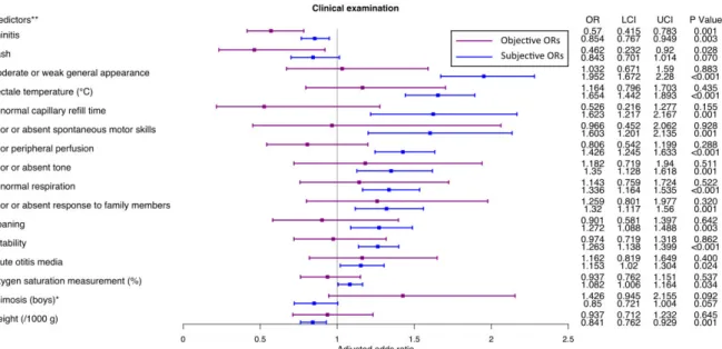
Estimating the probability that a patient has a disease is essential in the diagnostic process. Deviations from the accurate probability may lead to medical errors. Critically, a similar pattern of probability distortion has been observed in many domains (Zhang & Maloney, 2012). Small probabilities are overestimated and large probabilities are underestimated. Such S shaped distortion may have major implications for medical decisions by leading to either unnecessary or insufficient health care. Various studies have documented that cognitive biases and heuristics may affect diagnostic accuracy in medical decisionmaking. However, most of the studies are based on hypothetical medical situations (Blumenthal Barby & Krieger, 2014) and there is too little evidence of the impact on medical decision (Saposnik et al, 2016). To the best of our knowledge, probability distortion has not been studied in actual medical practice. In this article, we developed a method, based on the Lens model approach (Brunswick, 1952; Goldberg, 1970), to quantify probability distortion in actual clinical judgments and then assessed its impact on medical decisions. Probability distortion is commonly measured as the difference between stated subjective probabilities and controlled objective probabilities (eg, see Herrle et al, 2011). However, measuring probability distortion in the field raises methodological issues because the flow of information is not controlled as opposed to hypothetical medical situations. The first concern is the computation of objective probabilities. During the diagnostic process, physicians have access to a massive flow of medical features including but not limited to the medical history, the physical examination, and the clinical findings from laboratory tests.
synthesized in the literature (eg, see Van den Bruel et al, 2010; Van den Bruel et al, 2011), the values may not be available for all the features. Furthermore, medical features may not be conditionally independent (Holleman & Simel, 1997). Therefore, adjusted diagnostic values should be preferred to compute objective probabilities. A second concern is the use of stated subjective probabilities. The physician may take into account information that is not contained in the medical features. For example, it has been documented that physicians also rely on their clinical intuition (Van den Bruel et al, 2012; Woolley & Kostopoulou, 2013). Consequently, subjective probabilities may depart from objective probabilities if physicians use information that is outside the scope of the medical features used to compute objective probabilities. Our method requires an exhaustive collection of data from the field during the diagnostic process and a large number of observations. It is necessary to collect the medical features available for each patient (medical history, physical examination and clinical findings) but also to ask physicians, at the end of the diagnostic, to state their probability estimate that the patient has the disease and finally to know whether or not the disease actually occurred. From this exhaustive collection, two sets of predictors can be identified by stepwise regression: the predictors of the presence or absence of the disease (objective set) and the predictors of the probability stated by the physician (subjective set). Next, objective and subjective probabilities can be estimated by applying the corresponding regression weights to the objective and subjective sets of predictors respectively. Probability distortion is computed as the difference between the estimated subjective and objective probabilities. We applied our method to the detection of bacterial infection in febrile infants younger than
3 months (N=1848) and assessed its impact on two dimensions of heath care (antibiotic treatment and hospital admission).
Methods
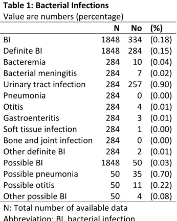
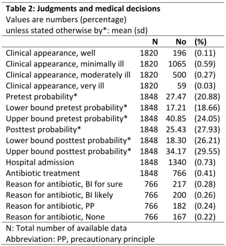
Study design, setting and participants Our data come from a study of the procalcitonin biomarker in the detection of bacterial infection (BI) in febrile infants younger than 3 months (Milcent et al., 2016). They performed a prospective, multicenter, cohort study in 15 French pediatric emergency departments for a period of 30 months from October 1, 2008, through March 31, 2011. Infants were eligible in the study if they were older than 7 days and younger than 91 days, with temperatures of 38°C or higher (at home or on admission), without antibiotic treatment within the previous 48 hours, and without major comorbidities (immune deficiency, congenital abnormality, or chronic disease). More details are reported in the original study (see Milcent et al., 2016). Data collection Physicians were asked to record the information they collected about the patient from its admission to its discharge. They recorded the demographic and neonatal data, medical history, physical examination, and clinical findings from ordered laboratory tests. Physicians were required to report their probability estimate that the infant had a BI, on a scale from 0 to 100%, and an interval within which their probability fell, at two stages of the data collection: (i) at the end of the physical examination (pretest probability); and (ii) after receiving the clinical findings from the laboratory tests (posttest probability). Following the
second estimate, they reported their decisions to hospitalize and to treat with antibiotics, along with a reason for using antibiotics (BI for sure, BI likely or precautionary principle). Study size Milcent et al. (2016) enrolled 2273 patients and 2047 infants were included in their final analysis. Furthermore, we restricted our sample to cases with available data regarding probability estimates and medical decisions and obtained a final sample of N = 1848 patients. Outcome measure The outcome measure included definite several bacterial infections and possible several bacterial infections categorized by the attending physician. Definite SBIs included bacteremia, bacterial meningitis, urinary tract infection, pneumonia, otitis, gastroenteritis, soft tissue infection, bone and joint infection. Possible SBIs included possible pneumonia and possible otitis. A committee of medical experts reviewed the diagnoses. Predictor variables We included all candidate predictor variables collected by physicians in the statistical analysis. Four categories of predictor variables were considered: (1) neonatal and demographic data, (2) medical history, (3) clinical examination, and (4) laboratory tests. We restricted laboratory tests to tests with clinical findings that were available when physicians were asked to report their second estimate, thus we excluded from our analysis blood culture, stool test and the procalcitonin assay. We also excluded additional samplings and additional radiography from the predictors.