The effect of a gap nonlinearity on recursive parameter identification algorithms

The Effect of a Gap Nonlinearity on

Recursive Parameter Identification

Algorithms

Scott E. Schaffer

SUBMITTED IN PARTIAL FULFILLMENT OF THE REQUIREMENTS FOR THE DEGREE OF

Master of Science in

Aeronautics and Astronautics

at the

Massachusetts Institute of Technology

May 1988

) Scott E. Schaffer, 1988

The author hereby grants to M.I.T. permission to reproduce and to distibute copies of this thesis document in whole or in part.

,. :Signature of Author

Department of einautics and Astronautics May 6, 1988

Thesis Sup- - "-- -

..

Prof. Andreas von Flotow . ;ronautics Accepted by

-c-- by.. Prof. Harold Y. Wachman

Z* <.C-Chawan, Department Graduate Comittee Aero

M.I.

Contents

1 Introduction

1.1 Background ...

1.2 Thesis Outline . . . .

2 The Nonlinear Model

2.1 Analytical Model.

2.2 Adaptation for Simulation .

3 Identification Algorithms

3.1 Choice of Domain and Algorithms ...

3.2 The RLS Algorithm.

3.3 The RLLS Algorithm... ...

4 Organization of Project

4.1 Choice of Forcing Function ...

4.2 Implementation of Algorithms ... 9 9 11 13 13 15 19 19 21 22 29 29 30

5 Results

5.1 Addition of the Gap Nonlinearity ...

5.2 An Analytical Comparison ...

5.3 The Effect of Noise on a Linear Model. ...

5.4 Combined Effects of Noise and Nonlinearity ...

6 Extension of the RLS Algorithm for an Explicit Nonlinear Model

7 Conclusions and Recommended Future Work

7.1 Conclusions ...

7.2 Recommended future work ...

A Derivation of the Voss RLLS Algorithm

B Relationship Between the Pseudoinverse and Kalman Filter

C The Fortran Programs

C.1 The Nonlinear System Model ...

C.2 The RLS Algorithm ...

C.3 The RLLS Algorithm. ...

C.4 The Extended RLS Algorithm. ...

33 38 41 45 49 53 53 57 61 71 73 74 75 76 77 33

List of Figures

2.1 Typical Load-Displacement Curve for Truss Structure. ...

2.2 Mass-Spring-Dashpot Model for System with Gap Nonlinearity...

3.1 Parameter Identification Procedure . . . . .

3.2 Lattice Effect of the Two Equations in the RLLS Algorithm ...

3.3 Component in the Blackwood experiment. ...

4.1 Forcing Function ...

5.1 Influence of the Gap Nonlinearity on Frequency,

Mass Estimates . ... Damping . . . . 14 14 20 24 27 30 Ratio, and . . . 36

5.2 Effect of the Gap Nonlinearity on the Convergence of the Mass Estimates. 37

5.3 Effect of Noise Parameter Gamma on the Convergence of the Mass Esti-mates ... 37

5.4 Effect of Noise on the Frequency, Damping Ratio, and Mass Estimates. 44

6.1 Extended RLS Estimates for Frequency, Damping Ratio, Mass, and Gap for Three Gap Sizes ... 51

A.1 A Graphical Interpretation of the RLLS Difference Equations ... 62

Abstract

This work examines the performance of the Recursive Least Squares (RLS) Algorithm and a derivative, the Recursive Lattice Least Squares (RLLS) Algorithm in matching a linear model to a simple nonlinear system. The response of a single degree of freedom mass-spring-dashpot system to continuous forcing is simulated, and estimates for the modal parameters are obtained. Nonlinearity is introduced by allowing the restoring spring to slide without friction in a gap of specified width. Such a nonlinearity is of interest since it is a simple model of the effect of loose joints in a deployable spacecraft structure. The effect of the gap size on the algorithms is studied, and the noise level and sampling rate are adjusted to see how they influence these results. The RLS Algorithm is found to be the most reliable. Finally, the RLS algorithm is extended to include an estimate for gap width, and good results are obtained for the noise-free case. Additional conclusions are made on how to minimize the effect of such a gap nonlinearity on the identification process.

Acknowledgements

I am grateful for the support of the following people, who made my time studying at MIT so pleasant:

Professor Andy von Flotow, whose inciteful questions during our discussions of my work were always able to show any flaws in my reasoning.

Gary Blackwood, who helped to make me feel at home in the Facility for Experi-mental Structural Dynamics, and who showed me how to make full use of the resources at MIT.

Erwin and Barbara Schaffer. my parents, who are always interested in my work and give lots of encouragement.

The members of the MIT Ballroom Dance Club, who provided a wonderful alterna-tive to studying seven days a week.

Notation

System Notation:

A average displacement amplitude c damping constant

k spring stiffness

M mass

u input (force)

y output (displacement)

yO location of boundary within gap y(O) initial displacement

Modal Parameters: w natural frequency damping ratio M mass 6 gap width Algorithm Variables:

a, a* coefficients of outputs in ARMAX form (RLLS)

e errors in equations (RLS)

e forward eqn errors, used as regressors (RLLS)

G forward coefficient matrix

{

bT

a*T

H backward coefficient matrix - (RLLS)

b*T

H unknown coefficients of parameters (RLS)

K, K* matrix of coefficients to regressors , e (RLLS)

i, k* Kalman gain factor (RLLS)

n number of steps in regression (RLLS) P, P* covariance matrix (RLLS)

p desired parameters (RLS) q-1 backwards time shift (RLLS)

r backward eqn errors, used as regressors (RLLS) z known quantities (RLS)

-y parameter for variance estimate (RLLS)

A forgetting factor (1.0 for no forgetting) (RLLS) (Note that starred variables indicate use in the backwards difference equation in the RLLS algorithm)

Method of Averaging Variables:

A The constant amplitude chosen for study

A(t) displacement amplitude as a function of time

ai small angle variables for use in computing boundaries change in phase angle as a function of time

Chapter 1

Introduction

1.1 Background

As man's experience with space has grown, the objects placed into orbit have become larger and more complicated. Current project designs will require an entirely new type of structure to provide the required surface area or volume. Large sensor arrays, wide mirrors for astronomy, and truss structures like the proposed space station all fall into this category of Large Space Structures (LSS). Several NASA experiments, including the MAST flight experiment and the COFS (Control of Flexible Structures) program,

deal with this this type of structure.

Accurate modelling of large spacecraft structures presents many novel difficulties. It is impossible to conduct full size ground tests of the structure because it is so large, and any finite element model is therefore of limited accuracy. Perversely, the need for active control of the structural dynamics makes accurate modelling necessary. One solution to this problem is to perform model or parameter identification, which when applied to structural dynamics is known as modal analysis. This involves the use of a computer algorithm to transform the motion of the structure into parameters that can be used in a model for control purposes. Experimental modal analysis of large spacecraft structures presents unique challenges, however. Because a structure in space cannot be secured, it will have several rigid body modes. A further complication is that the structure

may require the application of control forces, even while parameter identification is in progress. Lastly, since it is being assembled on orbit, it may include relatively loose joint hardware, designed to enhance ease of assembly. These joints introduce important

nonlinearity into the response. [11]

If modal analysis is used to analyze these spacecraft structures, it must have several important characteristics:

* Recursive. The algorithm must be capable of frequently updating the estimates of parameters, to allow the structure to be modelled even in the process of mod-ification. More importantly, recursive algorithms require less data storage, since they only work with the most current information. This more than compensates for then disadvantage that recursive (or 'on-line') algorithms usually do not give as accurate results as batch (or 'off-line) algorithms.

* Allow Input Superposition. To prevent rigid body motion or excessive deflections during the tests, control forces would have to be applied while the test was

con-ducted. Algorithms that require a specific forcing function (such as impulse or sinusoidal) could not be used.

* Robust. The algorithm must be able to perform in the presence of the nonlinearity introduced by the loose joint hardware, and give reliable estimates.

Recently, some time-domain parameter identification algorithms have been proposed which have the first two characteristics, but there has been little study of their perfor-mance in the face of nonlinearity. If these algorithms are to be used with confidence in a parameter identification process on a large spacecraft structure, this performance must be examined.

1.2 Thesis Outline

The most common type of nonlinearity found in the joint hardware of truss beams is a gap (deadband) nonlinearity. Therefore, in chapter 2, a simple model containing a gap nonlinearity is chosen and analyzed, and the equations of motion are developed. This nonlinear system will be used to test the identification algorithms.

Two Least-Squares based algorithms are chosen for study, a basic Recursive Least Squares (RLS) Algorithm, and a Recursive Lattice Least Squares (RLLS) Algorithm as formulated by Voss. These algorithms, along with other recursive algorithms, are clearly explained in a text by Ljung on recursive identification. [9] The basic theory of the chosen algorithms is explained in chapter 3. Chapter 4 then gives details on the implementation of the model and algorithms as part of the computer simulation, including the choice of forcing function and programming details.

The effect of the nonlinearity on the modal parameter estimates (natural frequency, damping ratio, and mass) are studied for both algorithms. The influence of noise, sampling rate, and (for the RLLS algorithm) the noise parameter 'y are also examined. These are detailed in Chapter 5. A linear relationship is found between the size of the gap and the estimated parameters. Noise, sampling rate, and choice of i are found to have a significant effect on these estimates. An attempt to improve the identification process is made by extending the RLS algorithm to include an estimate for the gap, and good results are obtained for the noise-free case. The results of this extension are shown in Chapter 6.

The RLS algorithm is found to be generally superior to the RLLS algorithm. Knowl-edge gained from studying the effect of the gap on the three algorithms leads to several conclusions of how to minimize the nonlinear effect on the identification process.

Chapter 2

The Nonlinear Model

2.1 Analytical Model

A truss structure assembled in space typically will have a static load-deflection curve as shown in Figure 2.1, indicating a gap (deadband) nonlinearity and slight hysteresis. In order to study the effect of this gap (without the hysteresis) on recursive parameter identification (PID) algorithms, a single degree of freedom mass-spring-dashpot model is chosen (figure 2.2).

The boundary of the system is allowed to move in a frictionless gap of arbitrary width, 26. This yields the following equations of motion:

M + cj + k(y - 6) =

(2.1)

Mi+cy+k(y+6) = u (2.2)

Myi = u (2.3)

c(- o) + k(y- yo) = 0 (2.4)

where (2.1) is for motion on the right side of the gap, (2.2) is for motion on the left side of the gap, and (2.3-2.4) is for motion inside the gap. The boundaries between the states occur when

FCE

TK)N

Figure 2.1: Typical Load-Displacement Curve for Truss Structure.

F= u(t)

or

¢

Y = Yo

-

(i - o)

where the stop location Yo = 6 at the right boundary and yo = -6 at the left boundary. The sign of the Yo term indicates the direction the system is moving across the boundary condition. This model has desired the type of Load-Displacement curve.

Since the parameters of interest are the modal parameters of natural frequency (w), damping ratio (), and modal mass (m), the equations of motion are rewritten using the identities c = 2wm and k = mrn2. This produces equations of the form

j

+ 2Swj

+w

_(y

_{_ ) =}

_u/m

ji + 2wj +w

_{(y + 6)}

_u/m

2.2 Adaptation for Simulation

In order to make these equations useful for computing a displacement history, they are changed to finite difference equations using the Central Difference Method. This method is chosen because of its simplicity, stability, and lack of numerical damping. This explicit integration method uses the following approximations for the derivatives:

1

i

So the equations cases. This gives

of motion may be written explicitly to solve for yt+At in each of the the final solution for the motion which the computer can solve:

[2 - (At) 2] yt + [-1

[2 - (wAt)2] t + 1-1

+ wALt] yt-at + -2 t + (At) 26

(1 + ~wAt)

+ gwat] yt-at + - 2 _{t - (t)} 2 ₆

(1 + gwAt)

At2

= 2

yt-ytAt+

= (WAt)

(Yt

-

yot) + (yt + t - yt-at + yot-at)

g(A;At

Note that the first two equations differ from the linear system equation by the term

(wAt)2

(1 + oWAt)

which may be thought of as a constant noise term, or as a disturbance force. The difference equations are used to calculate the displacement of the system at each time step t+At, based on the forcing and displacement history. This generates the pseudo-data which is used to test the parameter identification schemes.

In the actual algorithm, a slightly different formulation of the last equation was used. Letting the spring stretch q = y-o, = yi-io, where yo(O) = -6 and y(O) = -6- c(o)_k for the mass moving right in the gap, then q(0) = -c.

Since the equation of motion is

( - o) + k(y - o) = 0

This yields q(tg) = q(O) e-(kc) t, or

yo(tg) = y(tg) + c _k e(O) e(k/c) t

yo(tg) = y(tg) + ((t -5 - (t-_,t) e-(w/2)t.

This shows directly the exponential nature of the relaxation of the spring/dashpot element within the gap. It does however make the assumption that the system returns to equilibrium before touchdown on the other side. In retrospect, working with difference equations directly might be preferable. The displacement is updated in the gap as

At2 Yt+At = 2yt - Yt-A&t + -MUt.

The boundary conditions occur when y = So - (- to). Liftoff occurs from the left side when the mass was moving to the right, and yo = -6, io = 0:

2;

t+At

> -6- ,--t - yt-at)

Liftoff occurs from the right side when the mass was moving to the left, and yo = +6, Vo = 0:

t+t <

6

-

(t - Yt-at).

Initial conditions on the displacement are calculated by setting the initial displace-ment to y(O) and the initial force and velocity to zero. This yields:

t (y(1) - 2y(0) + y(-1)) + w2(y(0) + 6) = (0)

At2 M

For y(-1) s y(1) (at a minimum point),

8(l) = 1 [(2 - w2At2_{) y(O) + ((O) _ - 26) t2].}

Chapter 3

Identification Algorithms

3.1 Choice of Domain and Algorithms

Identification algorithms are designed to take the frequency response or time history of a system and from this information extract the parameters to fit a specific model. A flowchart of this process is shown in figure 3.1. These parameters can then be used to verify or update a model, improving the accuracy, to determine the effects of a structural modification, or to perform modal synthesis (determining the response of a structure based on the response of its components). Identification algorithms fall into two categories: frequency domain methods and time domain methods.

In the frequency domain, the equations of motion for a linear structural system are typically given as

[-w2M + jwC + K] y(jw) = u(jw)

or y(jw) = H(jw)u(j), where H(jw) is the frequency response function (FRF) matrix. Fullekrug [4] classifies the frequency domain algorithms into two categories: Sine-Dwell methods, which measure the resonance of a structure directly at its natural frequencies, and FRF techniques which measure responses for closely spaced discrete frequencies and use matrix techniques to extract the parameters.

AO PID

ALGORITHMS

A, , M

PARAMETERS

Figure 3.1: Parameter Identification Procedure

In the time domain, the equations of motion may be written as

MP + C; + Ky = u(t).

Fullekrug divides the time domain algorithms into those based on free vibration, and those using forced vibration.

Because for this project a recursive algorithm allowing force superposition was de-sired, the algorithms was chosen from the time domain algorithms based on forced vibration. These include such Least-Squares based algorithms as the Eigensystem Re-alization Algorithm (ERA) and Autoregressive Moving Average (ARMA) methods.

Two algorithms were chosen for study, a simple Recursive Least Squares (RLS) algorithm, and a Recursive Lattice Least Squares (RLLS) algorithm. The latter was chosen primarily because of its use for identification in a concurrent experiment by

Blackwood. [2] FORCING FUNCTION TIME HISTORIES SYSTEM

3.2 The RLS Algorithm

The RLS algorithm is simple in concept, since it is just a slightly modified form of the basic Least Squares formulation. The idea behind a least squares solution is simple. Given a set of equations which linearly involve a set of parameters, one may write them in matrix form: Zl Z2 Zn p11 421 4nl

...

If the number of equations exceeds the number of parameters (i.e. n > m), the estimated values for the parameters

0

This is referred to as the pseudoinverse. The relation of the pseudoinverse form to a kalman filter formulation is shown in Appendix B.

Since this algorithm is trying to fit the modal parameters of a linear system,

j + 2wj + w2y = u/M, the governing equation is put in the form

an=[-d2

n

-y

uit]

1/M

and evaluated at a sequence of instants to generate a matrix equation. Given the pseudo-data points of ui and yi, the values of ~w, w2, and 1/M are found that minimize the

squared error. The derivatives of y are calculated using the central difference method. The algorithm is made recursive by evaluating the contributions to the 3x3 TE and 3x1 KATz matrices at each time step and adding them to the existing values. The new

matrices are used to calculate new values of 0 for each i > 3.

3.3 The RLLS Algorithm

The RLLS algorithm is a linear, discrete time, state-space method. It is based on the ARMAX (Autoregressive Moving Average, Exogeneous inputs) form of the linear difference equation, which may be written as

y(t) = aly(t - 1) + blu(t - 1) +

+ ay(t - n) +

bnu(t

- n) +

bou(t)

+ en(t)

This form is also known as an estimator form, since the output is a linear combination of previous inputs and outputs, and may be used to estimate future output values for a system, as was done in simulating the nonlinear system (see equations 2.9 to 2.12). The ARMAX form has been used for many years on linear systems with excellent results, and the technique is commonly known as Linear Regression.

The RLLS algorithm offers several advantages. Besides being recursive and allowing input superposition, it has fast convergence for small data variance, and it can handle

many degrees of freedom simultaneously. A disadvantage is that it requires strong excitation of the natural frequencies, and so has difficulty with a pseudorandom input.

The RLLS algorithm is unusual because it also makes use of a backwards difference ARMAX equation:

y(t - n) = aoy(t) + bou(t) + ... + a*_ly(t - n + 1)

+bn-lu(t

- n + 1) + bu(t - n) + rn(t).

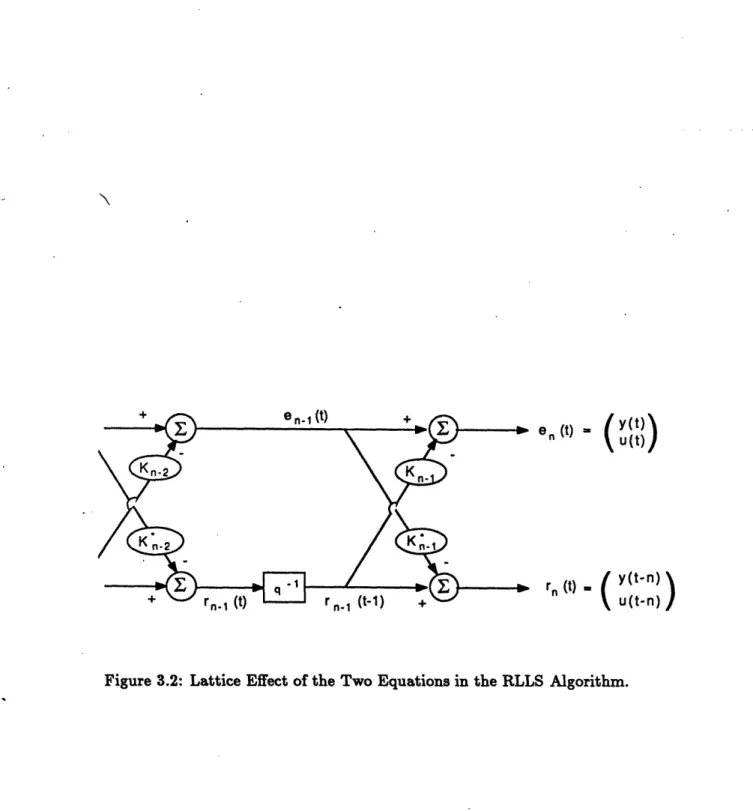
The two equations then go through a change of basis to make the error terms the regressing coefficients. This derivation is included in Appendix A. The result is a pair of equations which form a lattice (see figure 3.2):

u(t))

rnl(t - 1)

y(t-n)

(

u(t

-

n))

where Ki and K* are 2x2 vectors used as regressors.

!

Reflection Coefficient matrices and

eo(t - n + 1)

e(t- n + 2)

an-1 (t)

e, and r- are 2xl error

The Voss formulation of the algorithm makes use of two Kalman filters to solve for the values of Ki and Ki*. This reduces the number of computations required. According to Ljung [9], this type of formulation produces assymptotic convergence of the estimates with a zero mean, normal distribution, covariance matrix for the errors e and r. He also

r

I

K (t)

(t) ... X.-(t)

n (t) = y(t-n)

u(t-n)

mentions that while it works well using a sinusoidal input, it may be bad for white noise input. The Voss RLLS algorithm in algebraic form is included at the end of Appendix A.

Once the Ki and K* have been determined, the desired modal parameters may be extracted by examining the equations of motion in estimator form as computed through the Central Difference Method:

t (yt+,-t

-

_{yt + yt-At) + t(yt+t - Yt-t) (o)}

₊

_{Yt (w)}

₌

_ut().

2- 1t2t

+

+

1 + VoAt I + ¢woAtj 1+ AwoAt V

The parameters may then be extracted, since

yt+At = GlYt + G

ut + Gsyt-t

1-0

wo=

- /(2 - G(1+ wAt)

M

t

_/G

1+ wAt

The RLLS algorithm has been studied in several papers, mostly by Morf for linear models. [7,8] This algorithm has a number of advantages over the simpler RLS algorithm. Unlike the RLS algorithm, with which there is a penalty in accuracy for going beyond the true model order, the RLLS algorithm may be based on a model of arbitrary order. Additionally, all estimates provided by lower order models may be recovered, because only the new information provided by each increase in model order is used to change the estimates. The ability to overspecify the order enables an unknown system to be given

an arbitrary order (based on an overspecified number of degrees of freedom) and a good model obtained by seeing when the results cease to improve for a higher order. Another advantage for selecting the RLLS algorithm is that it it more computationally efficient for large models (n>5), since the computing cycle time is linear with the number of states, as opposed to a quadratic relationship for the RLS. Since our model system is small, this advantage will not be shown here.

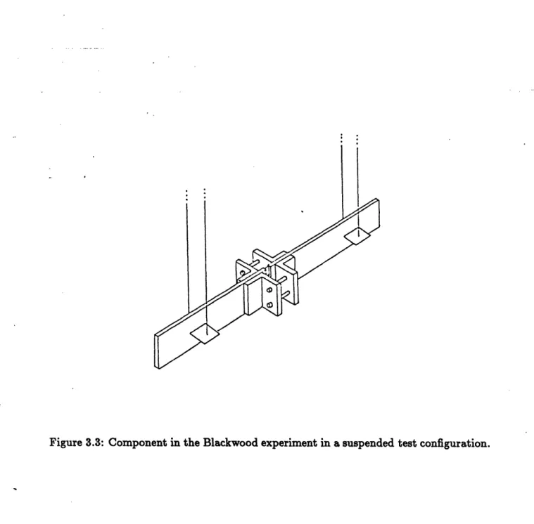
A final incentive for choosing this algorithm for study was its use for parameter identification in a concurrent modal synthesis experiment being conducted at M.I.T. by Blackwood.[2] This experiment involves the analysis of a real vibrating jointed beam with a gap nonlinearity. The bending modes of the beam are excited by a shaker apparatus, and screws at the joints may be adjusted to introduce varying amounts of gap into the joint. The experimental beam is shown in Figure 3.3. The spectrum analyzer for this experiment, a Signology SP-20, uses the RLLS algorithm.

Chapter 4

Organization of Project

4.1 Choice of Forcing Function

One of the most important criteria when choosing a forcing function is that it is 'per-sistently exciting', or excites all the modes that need to be identified. For his use of

the RLLS algorithm, Morf generally assumes that input is white noise. [7] The first forcing function chosen to excite the system was therefore a random input. This func-tion, however, did not excite the system enough to give good results, and the parameter estimates given by the parameter identification algorithms were different for each ran-dom function. Additionally, Soucy and Vigneron [11] recommend against use of ranran-dom forcing as tending to eliminate the nonlinearity through averaging.

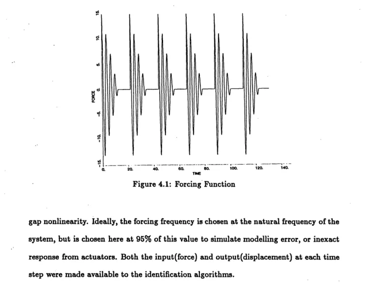
Therefore, the forcing function chosen for this work is a sinusoid in a linear envelope, repeated six times (See Figure 4.1). The basic function was determined by Voss 121 to be optimal for the RLLS frequency estimate, and it is repeated to give the mass

and damping ratio estimates time to converge. Too short a time makes the algorithms provide meaningless results for larger gaps, and the RLLS algorithm becomes very sensitive to choice of y. It was determined by trial that long term forcing, rather than free decay, was needed to give good estimates. This repetition gives better results than a single function with a longer envelope. This forcing function also gives a fairly constant displacement amplitude, which is important when analyzing the influence of a

I d Ii I 140. ThE

Figure 4.1: Forcing Function

gap nonlinearity. Ideally, the forcing frequency is chosen at the natural frequency of the system, but is chosen here at 95% of this value to simulate modelling error, or inexact response from actuators. Both the input(force) and output(displacement) at each time step were made available to the identification algorithms.

·4.2 Implementation of Algorithms

The RLS algorithm is simple to implement. The 3x3 matrix is inverted analytically, allowing the contribution at each time step to be added directly, rather than having to invert the matrix at each time step. The algorithm will not converge exactly in 3 time steps, even for a linear noise-free system, because the Central Difference Method includes terms for yt and yt-t but does not account for the force at the previous time step, ut-At, that relates the two displacements.

were caused by numerical instability in the form of roundoff error. It was determined that a change in the 4th decimal place of the input would change the first decimal place of the parameters. The problem was eased by using a UDUT formulation for the covariance matrix P, which factors the matrix into two triangular matrices and a diagonal matrix as suggested in references [9] and [12]. This formulation reduces the number of addition operations in the matrix multiplications, reducing the chance for roundoff error.

Another cause of delay was that the best sizes of the required values for the param-eters P(0) and 'y were ambiguously treated in the literature. P(0) is the initial value for the covariance matrix, which requires large values (see Appendix A). Values greater than 200000 x I2:2 yielded negligible improvement, so this was chosen. The parameter 7y is a scalar weighting factor used to account for noise in the data. More exactly, - = A\,

where A is the forgetting factor and 6 is the least squares weighting factor described in Ljung's book. [9] The specified initial value, -'0 = AV, is the forgetting factor times the nondimensionalized variance of the data noise. The forgetting factor is used to discount old data if the system is time varying. For our constant system, this parameter should be set to 1 for no forgetting. For a noise-free case, 'y could be set to zero, but because of numerical errors, a value of .000001 was found to be suitable. Voss claims that the best results for noisy data occur when V is set to 100 times the true variance.

Because of the forcing function chosen, it was also found necessary to modify the way that the mass parameter was calculated, since a contribution from the force at time t-At was identified. The force is changed from ut(1/M) to ut(1/M)(z) + ut-at(1/M)(1 - z) (since ut ut-&At). This splits the influencing force over the two time steps. In this case, since

G2 XAt2_{/M G (1- ) t}2_/M

Then the mass is

At29

(1 + fwoAt)(G2 + G4)' This yielded the correct mass for the linear noise-free case.

To non-dimensionalize the size of the gap, it should be divided by the total path length that the displacement covers. This was found by writing a FORTRAN program to keep track of the peak displacements. This program, along with the system estimation and parameter identification algorithms, is included in Appendix C.

The simulation was organized into three steps. First the forcing function was com-puted at discrete time steps. This was then used as input into the system to be studied, and a file of the resulting displacements was created. To simulate a sampling effect, the displacements were recorded for only every other time step. Last of all, both the force and displacement histories were fed into the parameter identification algorithms. Two different versions of the output could be obtained: either showing the identified parameters at each time step, to check things like speed of convergence, or giving all parameters at only the last time step, to save computing time when running through a large number of cases. These final values (after 40 periods) are the ones used in the results section.

Chapter 5

Results

5.1 Addition of the Gap Nonlinearity

The specific parameters:

system used for the simulations has the following

k = 20 N/m c = 0.4 N-s/m M = 5.0 kg y(0) = -2 m w = 2/sec g = .02 6 = specified Period = r

This is then forced by the function

u = 15 (1 - .08t) cos (1.9t)

repeated every seven periods, for a total of 42 periods (total time 132 sec).

The standard sampling rate is 30 per period. It is found that at higher rates (such as 60 per period) the RLLS Algorithm proves to be very unstable with the parameter 7, even with the UDUT and Kalman Filter formulations. The sampling rate chosen proved to be much more stable, probably because of smaller numerical roundoff errors. It should be mentioned that the RLS algorithm does not suffer from these numerical difficulties, and its accuracy improved with the increased sampling rate, but not enough to warrant using different rates for each algorithm.

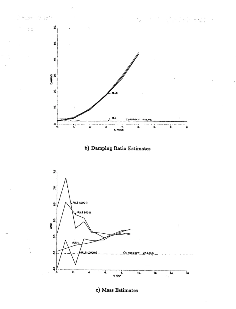
The influence of the gap nonlinearity is studied by use of the nondimensional ratio of 6/ A (gap size/average amplitude). This particular ratio is chosen because it determines the fraction of the displacement amplitude that passes through the gap. With this choice, when the gap size approaches zero or. the amplitude becomes very large, the results approach those of the linear system. The final estimates for each of the three

parameters are plotted versus 6/A in figure 5.1.

CORRCTr VA-LO-Ct0001) o. 2. 4. 6. . 10. 12. 14. 16 GAP a) Frequency Estimates y, I -- _ ., _ . . - , _ . ... I

d a C5 I8 a; d d % NOISE

b) Damping Ratio Estimates

oo0l

Woo)

SGAP 1 12.

c) Mass Estimates

Figure 5.1: Influence of the Gap Nonlinearity on Frequency, Damping Ratio, and Mass

L

Iq

l

l

The RLS algorithm shows a linear decrease in the estimates for the natural frequency and damping ratio, and a linear increase in the mass estimate as 6/ A increases. The RLLS algorithm gives the same results for frequency, since the forcing has been opti-mized for this estimate. The RLLS mass and damping estimates are highly dependent on the choice of for small gaps ( 6/ < 5%), but converge to the RLS estimates for larger gaps. Approximate linear equations for the RLS estimates are:

= (.997- .54 6/i)

Sc =

(.980-1.886/A)

These may be used to adjust a linear model to account for a gap. They also could be used to estimate the size of the gap, given a variation between the linear model and the estimated parameters, but surely there are better ways to do this.

At first it seemed that the RLLS estimates were more consistent with increasing

6/ A because the system was being forced more closely to its natural frequency (i.e. the

natural frequency had dropped to 95% of the linear value because of the gap). However, changing the forcing frequency does not change the trend. Examination of the time traces (see figure 5.2) shows that the estimates for larger gaps converge more quickly. This faster convergence probably comes from what the algorithm sees as increased variance in the data relative to , the variance parameter, since it is noted that smaller values of y (for the same gap size) also make the estimates converge more quickly (see figure 5.3). This will lead to an investigation into the effect of noise on the RLLS estimates.

TIME .,

Figure 5.2: Effect of the Gap Nonlinearity on the Convergence of the Mass Estimates.

d

20.

Figure 5.3: Effect of Noise Parameter Gamma on the Convergence of the Mass Esti-mates.

asa~

sn (;Cy.~so

5.2 An Analytical Comparison

The effect of the gap nonlinearity on the natural frequency of the system may be esti-mated analytically using the method of averaging. The system is cast in the form

i + oo4y

= f(Y,O),

where

f(y, ) = -2woy + 026

f(y, j) = -2woj - w26

f(YY) = wo2Y

for the right side, left side, and inside of the gap (stipulating an unforced system).

A solution is assumed of the form

y(t) = A(t) cos +(t)

+(t) = ot + (t)

j(t) = -A(t)wo sin +(t).

Then, in terms of

4,

f(A(t) cos (t),-A(t)wosin +(t)) = 2wo A(t)sin +(t) + wO6

= 2owo A(t) sin 0(t) - Wo86

= w A(t) cos (t)

for the right side, left side, and inside of the gap.

Assuming that A(t) and +(t) can be treated as constants over one period, the bound-ary conditions are calculated in terms of

4'.

displacement. Using small angle assumptions, the following identities are determined: cos(ff/2 - al) a1 cos(3r/2 + a2) # -a2

cos(3wr/2 -

a3)

sin((7r/2 - al) 1 sin(ir/2 + a2) 1

sin(3?r/2

-

1

sin(32r/2

+

1-.

As the phase goes form 0 to 2r, each liftoff and landing condition is encountered. Since the liftoff and landing moving left occur at 6 - 2 y and -:

A(t) cos q(t) = y(t) = 6 - [-A(t)wo sin +(t)]

6 + 2SA(t)

+(t) = r/2- A(t)

and

A(t) cos(t) = y(t) =

-6

+(t) = /2+ A(t)

Similarly, the liftoff and landing moving right occur at -6 - 2L y and 6:

A(t) cos +(t) = y(t) = -6- 2 [-A(t)wo sin +(t)]

+(t) = 3r/2 + _A(t)2AA(t)

and

A(t)cos4(t) = y(t)= 6

+(t) = 3/2 +

The values for A(t) and p(t) may then be calculated from the following equations:

A(t)

= 2ro 2 f(A(t) cos (t), -A(t)wo sin (t)) sin (t) doL

(t) = 2To A(t) f(A(t) cos(t), -A(t)wo sin (t)) cos (t) do

If t is chosen at a point when A(t) = A, a constant, this yields -1

f(t) = 2?rwoA

o'/2 -A-+(2fwo2 A(t) sin 4(t) + wo26) cos (t) do

+ /2+__ (woA(t) cos 0(t)) cos

+(t)

1r/2+ -t +2t

+

f/2+itA

jr/2+ )

+ _{3X/2+ +2f}/2 ( (woA(t) cos4(t)) cos (t) do

2T

+ /2+

The solution is then:

(2wo2A(t) sin +(t) + wo25) cos +(t) do

or (for (0) = 0)

=- 06t.

IrA

The linear relation between natural frequency and gap size can then be shown by looking at the phase equation:

o(t) = wot- W t_IrA

= Wo(- )t.

IrA

Thus = wo(1 - .318-). This has a slightly flatter slope than that obtained from the algorithm, but still shows the linear relation.

(5.1)

(5.2)

5.3 The Effect of Noise on a Linear Model.

If the gap nonlinearity is indeed seen as adding noise to the system, a study of the effects of noise on the linear model is important. Noisy displacement data is produced by adding a random perturbation to the sensed displacement at each time step. The maximum amplitude of this noise is proportional to the average displacement amplitude,

Ay = NA. The proportionality constant N is referred to here as the percent noise. The

noisy data is then passed to the two parameter identification algorithms.

This noise is found to have a very large impact, since the estimates of Least Squares-based algorithms have bias errors with correlated noise.[10,12] The modal parameter estimates are plotted versus percent noise in figure 5.4. The RLS algorithm shows quadratic increase in frequency and mass estimates, and quadratic decrease in the damping ratio estimate. The RLLS algorithm shows quadratic increase in frequency and damping estimates, and an inverse relationship for the mass estimate. For esti-mates to be within 10% of the true values, noise has to be under 5% for the RLS and under 1% for the RLLS algorithm. The mass estimate is the limiting factor in both cases. It is noted that the addition of noise also makes the algorithms converge slightly faster, and makes the RLLS algorithm less sensitive to 7. This is to be expected if the gap is treated as an increase in noise, verifying this hypothesis.

The two algorithms yield the same results when the parameter a in the RLLS algo-rithm approaches zero (for the noise-free case). This agrees with theory, and is true as long as the initial estimates are zero.[3]

Adjustment of the parameter can be made to compensate for the increase in frequency due to noise, with very small values being best in the noise-free case and larger values needed as the noise is increased. Setting -y = 0 does not yield a convergent

estimate in the noise-free case because of small numerical errors, so a value of y = .000001 is chosen. Voss' rule of thumb of 100 times the true variance seems to work only for percent noise under 1%, since it was found that for 1% noise the best value is .0001 and for 5% noise it is 4.0. The choice of a larger value of My allows more data to be processed before the estimates converge, allowing the algorithm to compensate for the noise. The parameter, however, is unable to compensate for the very strong changes in damping ratio and mass estimates with increasing noise. These estimates would have to be normalized somehow for the parameter to affect all the estimates. Without a priori knowledge of the modal parameters, this would be difficult.

R.LS ; t1) Co _ R-EC VYL _ _ . _ . 1 _ ._ _. .-- _ --- _ _ . 1. 2 3& 4. & a 7 a % NOISE a) Frequency Estimates 0. !

10 12Z 14. 6.

b) Damping Ratio Estimates

0. 1. 2. 3 4. 6 A NOISE

& 7. 8

c) Mass Estimates

Figure 5.4: Effect of Noise on the Frequency, Damping Ratio, and Mass Estimates. (' 0 I eq q FL u I "-% GAP-. .. I

5.4 Combined Effects of Noise and Nonlinearity

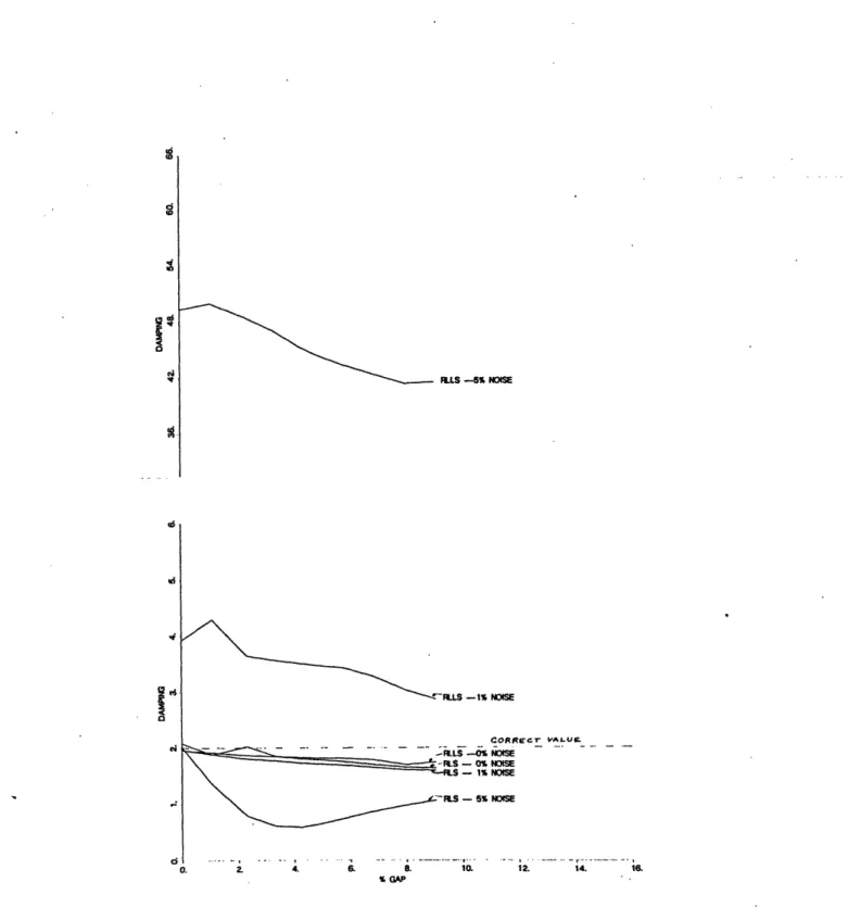
The prior sections summarize the effect of measurement noise and nonlinearity when each is present. The effects on the parameter estimates are, in part, in opposite direc-tions. The next step is to determine the effect on the estimates when both noise and nonlinearity are present. It turns out that when noise is added to the nonlinear data, the curves for the variation of parameter estimates with gap are shifted accordingly, as shown in figure 5.5. Here, only the optimal value of -y for each noise level is used (.00001 for linear, .0001 at 1%, 4.0 at 5%). Low noise levels produce the same linear increase or decrease (higher noise levels have a greater deviation in shape, probably due to incomplete convergence). This shows that the effects due to the gap and the noise can be superimposed. A small amount of noise can completely offset the drop in frequency due to the gap.

cV- VAL-E . NOISE HNOSE NOISE N USE NOISE % GAP 12. 14. 16. a) Frequency Estimates RLS - 5% NOISE / ,.-LS - 1 NOtSE ILLS-OX SE -tS - 0% NOISE CO R E Gr -RLLS -5% NOISE

_~~~~~~~~~~onL

ILLS -5% NOISE -RILS -1% NOISE CORRcr VALULF-... \ . . . .. -IS - 1% WISE \ as - 5% NOS

...

...

....

, , ,....

...

c) Damping Ratio Estimates'

Figure 5.5: Effect of Noise on the Estimates for a System with a Gap Nonlinearity.

0 ED 0" v, i ED 2 C4 C A X d .I

Chapter 6

Extension of the RLS Algorithm for an Explicit

Nonlinear Model

The RLS algorithm may be extended to include an estimate for the size of the gap itself. This type of extension will work for any linearity that adds extra terms to the equation of motion, such as a cubic or quadratic nonlinearity. The new matrix formulation is

fS

=[2

v u ±11

1/M

602

This is solved as the RLS algorithm was, through use of the Central Difference Method to compute the derivatives, and extracting the parameter estimates through the pseu-doinverse. The actual program used is included in Appendix C. As indicated in the equation above, it ignores the data within the region of the gap, -E < y < 8.

This algorithm produces very good results for the noise-free case, regardless of the size of the gap. In fact, the parameter estimates become slightly more accurate as the gap increases. In the presence of noise, however, (since this algorithm is also based on a Least Squares formulation) a strong bias is introduced. These results are shown in figure 6.1.

4.3% GAP LINEAR 1.0% GAP VALUE: 0o. 2. 4. 6. o. % NOISE

a) ERLS Frequency Estimates

d .i a; 6 c i 4. . . o . . ,

b) ERLS Damping Ratio Estimates

12. 14. 16. LINEAR 1.0% GAP ,43% GAP CO R Cr ALUE. 1n 12 14 lv 0. 2. 9 o C '^ iu. c

43% GAP

1% GAP

ULEAR

. -. 6 - . 1. _-- , -__ ,

1 IZ 14. la

c) ERLS Mass Estimates

1D% GAP -.- COARRE r VALUcS . j d 0 -- .. - -. , . .. .. .. O. 2. 4. & IO 12 14; % NOISE 16

d) ERLS Gap Estimates

wd (4 w d I,-M 9 % NOISE. .

Chapter 7

Conclusions and Recommended Future Work

7.1 Conclusions

A gap nonlinearity, such as would be found in an assembled truss structure, has a very definite effect on parameter identification algorithms. Increasing the gap size produces

a linear decrease in frequency and damping ratio estimates, and a linear increase in the mass estimate for both the RLS and RLLS algorithms. The gap does not cause the algorithms to fail, because both simply fit the best linear model they can. Additionally, the gap causes faster convergence of the estimates, and makes the RLLS algorithm less sensitive to choice of the noise variance parameter 7.

The addition of noise to the data also produces faster convergence and less sensitivity to y. Noise however causes very large bias errors in the estimates, and these are in the opposite direction to the change caused by a gap. These large biases are probably not seen in the results for the gap nonlinearity (figure 5.1) because the gap is seen only as a low frequency, constant amplitude disturbance. While the Central Difference Method used in the algorithms differentiates the noise, making it worse, the constant amplitude error from the gap differentiates to zero. Since bias errors for the gap are probably small, the drop in frequency and damping ratio noted with increasing gap should accurately reflect the average system parameters. Use of the method of averaging showed this same type of linear decrease in frequency.

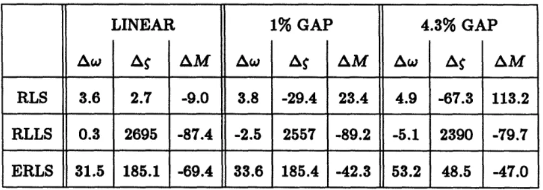
The effect of 5% noise on the three algorithms is shown in Table 7.1. The optimal values of the variance parameter 7 are used throughout. The frequency estimates of the ERLS algorithm in the presence of noise are consistently worse than those of the RLS and RLLS algorithms, but the damping and mass estimates are better than those from the RLLS algorithm, and become better than those from the RLS algorithm with higher gap size. The RLS and RLLS results are comparable in the magnitude of the frequency estimate error, but the RLS yields far better estimates for the other parameters. In general, for moderate noise levels, the RLS algorithm is the best choice of these three. For low noise levels and significant gap, the ERLS Algorithm would be preferable.

Table 7.1: Comparison of the Effect of 5% Noise on the Algorithms. Given

as a percent change from the noise-free value of the estimates.

An additional reason that the RLS algorithm is preferable to the RLLS algorithm is that the RLLS algorithm is too sensitive to the noise variance weighting factor and to finite roundoff errors. Therefore, certain gaps sizes do not mix well with choices of 7, as was found for the choice of 7 = .0001 at the 1% noise level with a 4.3e% gap. Numbers around this unstable point yielded worthless answers as the algorithm could not converge. While a faster sampling rate improved the performance of the RLS

LINEAR 1% GAP 4.3% GAP

Aw A S AM Aw A AM Aw A AM

RLS 3.6 2.7 -9.0 3.8 -29.4 23.4 4.9 -67.3 113.2 RLLS 0.3 2695 -87.4 -2.5 2557 -89.2 -5.1 2390 -79.7 ERLS 31.5 185.1 -69.4 33.6 185.4 -42.3 53.2 48.5 -47.0

algorithm, it only aggravated the problems in the RLLS algorithm.

The noise problem can be dealt with in a number of ways. The easiest way is to use one or more low pass filters, to eliminate the noise before it enters the algorithms.

Another common method is to overspecify the number of degrees of freedom in the RLLS model for the system, allowing the algorithm to fit the noise to high frequency modes. In this case, the RLLS algorithm may work better, since the system is easily overspecified and the improvement with each extra degree of freedom may be examined without running the algorithm again. There is an entire class of Least-Squares based algorithms that are designed to handle the bias due to noise by increasing the dimensions of the matrices to include the magnitude of the error due to noise. These are referred to as Extended Least Squares algorithms. Finally, it is probably better to use acceleration data and integrate for the other variables, thereby minimizing the noise effects rather than increasing them.

If a detailed model including the gap is desired, the ERLS algorithm as written in this thesis may be used, or another algorithm may be similarly modified. This gives very accurate results in the absence of noise. There are also a number of algorithms which use different approaches to get a value for the nonlinearity directly. The Kalman filter may be extended to include a nonlinearity. In the Bayesian form [9], the parameter is thought of as a random variable, and a solution is given as a probability density function for the states. Billings [1] expands the nonlinearity into sines and cosines and obtains a linear model. Others, such as the Threshold Adaptive Modelling Technique [5] or Volterra and Wiener Series use a complicated kernal formulation and are quite recent. They seem to show promise when used with complex nonlinearities like a gap.

effect of the gap on the identification process can be minimized. It is important to use a continuous forcing function, since in free decay the size of the gap relative to the average displacement amplitude is always growing, leading to constantly greater distortion of the results. The frequency content should excite all the desired modes, and the amplitude of the displacement should be relatively constant. While it would be nice to force the displacement amplitude to be as large as possible (since this minimizes the numerical problem and the nondimensional gap and noise sizes), it is preferable that the displacement amplitude matches that which the system is expected to encounter during use. In this case, the linear nature of the frequency drop may be exploited in that only two or three amplitudes need to actually be tested, and a linear plot of frequency versus displacement amplitude can be drawn. This would allow a switch between models at different amplitudes for best results. The forcing needs to continue for a long enough time (here 42 periods was chosen, and this is probably a minimum) for the algorithm to converge.

It may also be noted that the higher the damping ratio, the more accurate the damping ratio estimate. This was found in a separate project, not discussed here. The effects of a gap can be eliminated entirely by loading the structure in compression (or tension), and never allowing the displacement to cross the region of the gap. This is sometimes done in practice.

With precautions, parameter identification of a system with a gap nonlinearity can be conducted, and very good results obtained.

7.2 Recommended future work

This study of the effect of a gap nonlinearity on parameter identification could be followed up in a number of ways.

1. Higher Degree of Freedom Model. A model consisting of two or more degrees of freedom, each containing a gap nonlinearity could be studied. This work could be related to the modal synthesis of the Blackwood experiment. It could be determined whether it is better to include the nonlinearity as a disturbance force 7 = k6 instead of a change in displacement. Additionally, a better sense of how the gaps interact over the entire structure would be obtained.

2. Reliability With Other Nonlinearities. A model containing hysteresis, as well as a gap, or a model with a cubic nonlinearity included could be tested. This should give a better indication of how the algorithms would work in actual use.

3. Use on Real Structure. The algorithms need to be tested on a real nonlinear struc-ture, to determine the accuracy of the estimates compared to those obtained by

other test methods.

4. Study of Noise. Some of the ways to minimize the effect of noise on the algorithms could be studied, including the addition of noise modes or the use of an Extended Least Squares formulation of the algorithms. Further study on the effect of differ-ent types of noise could be done analytically, as Longman has done for the ERA algorithm. l10] The interaction of a Minimum Model Error (MME) state estimator

[7] with noisy gap data would be another interesting line of work.

5. Extension of Studied Algorithms. The RLLS algorithm could be extended to in-clude an estimate for the gap, as was done in this thesis for the RLS algorithm.

The Extended Least Squares form mentioned above could be used.

6. Study of Additional Algorithms. Study of the effectiveness on a gap nonlinear system of the ERA, or a nonlinear identifying algorithm could be undertaken.

Bibliography

[1] Billings, S. 'Identification of Nonlinear Systems - A Survey.' Proceedings of

IEEE, vol. #127, part D (Nov 1980) p.2 7 2.

[2] Blackwood, G.H. and A.H. von Flotow,'Guidelines for Component Mode Synthesis of Structures with Sloppy Joints.' 29th AIAA/ ASME/ ASCE/ AHS/ ASC

Structures, Structural Dynamics and Materials Conference, #3 (April,

1988) p.1 5 6 5.

[3] Brown, R.G., Introduction to Random Signal Analysis and Kalman

Fil-tering. John Wiley & Sons, 1983.

[4] Fullekrug, U. 'Survey of Parameter Estimation Methods in Experimental Modal Analysis.' 5th International Modal Analysis Conference, #1 (April 1987) p.460.

[5] Hsieh, S. and H. Lai, 'Threshold Adaptive Modeling for Drilling Dynamics Charac-terization and Process Monitoring.' 5th International Modal Analysis

Con-ference,#2 (April 1987) p.1 5 8 6.

[6] Juang, J. and R. Pappa, 'An Eigensystem Realization Algorithm (ERA) for Modal Parameter Identification and Model Reduction).' AIAA Journal of Guidance, Control, and Dynamics vol.#8 (Sept-Oct 1985) p. 620.

[7] Mook, D. and J. Lew, 'A Combined ERA/MME Algorithm for Robust System

Re-alization/Identification.'

29th AIAA/ ASME/ ASCE/ AHS/ ASC

Struc-tures, Structural Dynamics and Materials Conference, #3 (April, 1988)

p.1 5 5 6.

[7] Lee, D., M. Morf, and B. Friedlander, 'RLS Ladder Estimation Algorithms.' IEEE Transactions ASSP 29, #3 (1981) p.6 2 7.

[8] Lee, D., M. Morf, and B. Friedlander, 'Recursive Ladder Algorithms in ARMA Modelling.' IEEE Transactions AC-27, #4 (1982) p.7 5 3.

[9] Ljung, L. and T. Soderstrom, Theory and Practice of Recursive Identifica-tion. The MIT Press, 1983.

[10] Longman, R.W., and J.Juang, 'A Variance Based Confidence Criterion for ERA Identified Modal Parameters.' Paper # AAS 87-454, AAS/AIAA Astrodynamics Specialist Conference, August, 1987.

[11] Soucy, Y. and F. Vigneron, 'Identification of Structural Properties of a Continuous Longeron Space Mast.' AIAA 84-0930, 1984.

[12] Voss, J. E., 'Real Time Identification of Large Space Structures.' MIT Ph.D. Thesis, February, 1987.

Appendix A

Derivation of the Voss RLLS Algorithm

A RLLS algorithm is based on the interaction of two linear difference equations in ARMAX (Auto-Regressive, Moving Average, Exogeneous inputs) form. The first is called the forward difference equation:

y(t)

= aly(t - 1) + blu(t

- 1) + -.. + ay(t - n) + bnu(t

- n) + bou(t)

+ en(t). (A.1)

The terms y(t) and u(t) indicate outputs and inputs at time t respectively, so that the current output depends on a linear combination of the previous inputs and outputs. The variable n indicates the finite number of previous time steps, and is known as the order of regression. The term en(t) is the error between the linear approximation of order n and the actual y(t). This form of the equation is also known as a linear regression.

The second equation is known as the backward difference equation:

y(t-n) = aoy(t)

+ bou(t)

+ + an_ly(t-n + 1) + blu(t-n

+ 1)

+bnu(t - n) + rn(t).

The equations are shown graphically in figure A.1 below. Since the format of each equation is similar, only the forward difference equation is treated for now.

The ARMAX equation may be written in a matrix form:

i _ i_ ....-

_

..

I _

_

o

*

o-2

i- i

Figure A.1: A Graphical Interpretation of the RLLS Difference Equations.

Y(t - 1) u(t - 1)

y(t) =

. al , on

]

en(t)

where is then the vector of unknown coefficients a and b and is a vector of the previous outputs and inputs. One way to solve this type of equation is through use of a Kalman filter, which computes the unknown based on the following state space representation:

0(t + 1) = (t)

y(t) =

T(t) 0(t) + e(t).

This shows explicitly that (t) is made up of values which are constant for all time t. Note that T(t) (p(t) = (oT(t) 0(t) since both variables are vectors.

A more general state space equation is written as

x(t + 1) = F (t) + G u(t) + w(t)

y(t) = H x(t) + I u(t) + e(t)

This general state-space equation yields three iterative equations to solve for x(t) =

E(z(t) y(O),u(O),..., y(t-n), u(t-n) ) (an equation indicating that x(t) is an estimation

based on the previous data),

:(t + 1) = F(t)&(t) + k(t) [y(t) - H(t) (t)]

F(t)P(t)H

_(t)

H(t)P(t)HT(t) + r

(t)

P(t + 1) = F(t)P(t)F

_{(t) + ri(t) - k(t) H(t)P(t)F}

_(t).

This is known as a Kalman filter, k(t) is known as the Kalman gain. The parameters rl and r2 come from the 2x2 matrix of variances, R, where rl = E(w(t)wT_{(t)), r2 =} E(e(t)eT(t)) and rl2 = E(w(t)eT_{(t)). Since the errors are independent, rl2 = O. P(t) is} then the diagonal covariance matrix (the inverse of R). The derivation of these equations may be found in Ljung [9].

For our specialized case, F = 1, H = (oT(t), G = I = 0, x(t) = 9(t), and the first error rl(t) = 0. This yields the following three equations:

O(t +

1) = O(t)

+ k(t)[y(t)-

,(

k(t

PT(t)P(t)jo(t) + r2(t)

P(t + 1) = P(t) - k(t) PT(t)P(t)

This formulation is equivalent to the least squares solution if the system is overdeter-mined, the state is assumed constant, and no prior knowledge of the state is assumed. Although this is surprising, given that the least squares solution is deterministic, and the Kalman filter is a stochastic system, this is proved in Appendix B. The Kalman filter has the advantage that the initial state can be assigned a value, perhaps from a model. This speeds convergence.

The advantage of the RLLS formulation is that the effect of changing the regression order n on the estimate is made explicit. This allows the number of degrees of freedom

in the model to be overspecified, and the increase in order examined to see when no further improvement occurs in the parameter estimates. Additionally, the estimates for all orders less than n may be extracted, as opposed to the normal Kalman filter, which would require recomputing all the coefficients. The resulting form has the shape of a ladder (or lattice) as was shown in Chapter 3.

In her thesis, Voss makes maximum use of the Lattice properties and of the power of the Kalman filter by using an individual Kalman filter for both the forward and backward equations. She also modifies the notation used, in order to improve the algorithm's performance. She expands the basic equation (A.1) to include the current input as well as output, and defines a new variable i(t), where 1(t) = [ yT(t) uT(t) ]T. This requires the assumption that y(t) is not affected by u(t), which simply means that

there are no instantaneous effects on the system displacement. This yields the matrix equation (t) =

y(t)

i

1

y(t-n)

u(t

(

en(t)

j

)

There is a similar equation for the backward difference equation. This arrangement is made so that inputs and outputs may be paired at each time step. No attempt is really made to estimate the force u(t), so the values of c and d are essentially meaningless. Note that although the algorithm is usable for multiple inputs and outputs, I will only be using it for the single-input, single-output case, so that .(t) = [ y(t) u(t) T.

The two RLLS equations then become

(A.3)

for the forward direction, and

(A.4)

for the backward direction. The hat () indicates the variable being estimated. Note that G and H here are not the same as the coefficients in the general state space equation. Here the first row of G is . The composition of H is similar in size and meaning. The notation x(n)(t) merely indicates that the recursion order is n, and has no effect on the value of x(t).

The vectors O(n)(t - 1) and (n) (t) are defined to be

x(t- 1) (t)

(")(t - )= (t-2) ()(t) = i-1)

(it-

n)i h

t- n

+ l)

The superscript n continues to indicate the total time steps needed.

I

(A.5)

The equations A.3 and A.4 then undergo a change of basis, so that the errors en(t) and r(t) become the regressing terms, rather than z(t). Since

rE(t) rn (t) (A.6) (A.7) = (n) (t) - (n)(t) (n) (t- 1)

(=

x? (t-,n)

-

i(n)(t)

+(n)(t)

If G(0)(t) and H(0)(t) are set equal to a zero 2x2 matrix for all time t, then

(A.8)

izn)(t) = 6 ()(t) (n) (t _ 1) + n(t)

,(n (tn-I) y (n) (t) ±n) (t) + (t)

which is simply the data taken at time t.

The equation A.8 may then be written in matrix form, which shows the change of basis: ! 1% ro(t- 1) El(t- 1) r_-I(t- 1) / . I2Z2 0 ... -H(1)(t- 1) I22 .. -- ()-1)(t-1) -0 0 2z2 !

x(t-1)

x(t-n)

= T() (t- 1)

which makes use of the definition of (n)(t - 1) in equation A.5, and also equation A.7.

From this, choose a matrix K partitioned in the form

K=[K K ... Kn-1]

where the Ki are the reflection coefficient matrices, which are square matrices of dimen-sion equal to number of rows in x (2 for a SISO system). Define K to be

K = T

_h

so that in the new regressors (from equation A.3),

(G(n)(t) T-1)(T (n)(t - 1)) + en(t) _0(t- 1

[

rn-l(t

-Knl(t) tn-l(t-1)+ en(t)

This equation is easier to work with, since only one regressor, rn(t - 1), is needed at a time, making it much more suitable for an algorithm. The covariance matrix P

I r

I I

.1