FLOW SIMULATIONS IN POROUS MEDIA
Margaret S. Edie
Earth Resources Laboratory
Department of Earth, Atmospheric, and Planetary Sciences
Massachusetts Institute of Technology
Cambridge, MA 02139
John F. Olson
CLAM Associates
215 First Street
Cambridge, MA 02142
Daniel R. Burns, and M. Nafi Toksoz
Earth Resources Laboratory
Department of Earth, Atmospheric, and Planetary Sciences
Massachusetts Institute of Technology
Cambridge, MA 02139
ABSTRACT
Realistic simulations of flow in porous media are dependent upon having a three-dimensional, high resolution image of pore structure which is difficult to obtain. So, we ask the question, "How fine a resolution is necessary to adequately model flow in porous media?" To find the answer, we take a 7.5 p,m resolution image and coarsen it to five different resolutions. Lattice gas simulations are performed on each image. From the simulation results, we observe changes in permeability and velocity fields as the resolution is altered. The results show permeability varies by a factor of 5 over the resolution range. Flow paths change as the resolution is changed. We also find that the image processing has a large impact on the outcome of the simulations.
INTRODUCTION
How fluid flows through a complex porous medium has been studied by hydrologists monitoring groundwater, chemists tracking soil contamination, petroleum geologists trying to extract more oil from reservoirs, and geophysicists studying the flow of mantle melt through the Earth's crust. Despite many years of research, it remains a difficult question to answer because the medium is opaque and the process cannot be observed directly.
Laboratory and field experiments have been designed to try to understand how fluid moves through a matrix of rock or soil. Bulk parameters such as permeability, conductivity, and average velocity can be measured, but we can only guess at the details of the motion taking place inside the sample. However, the development of computer-simulated fluid dynamics has created a setting where flow at the microscopic level can be explored virtually. In order to perform such simulations using realistic models of pore space and thereby relate simulations to laboratory measurements on real rocks, it is necessary to obtain detailed digital images of the pore geometry of geologic samples. Gathering three-dimensional images of this kind is a difficult task and the techniques that have been tried have had mixed results. The ideal image would have high resolution so that small pores could be observed, and would cover a large enough volume for flow
properties to be meaningful. However, methods that yield very high resolution are
usually limited to imaging only small volumes. Therefore either a small volume at
high resolution or a larger volume at low resolution must be used. The latter was the
case in previous work done with NMR images, where the resolution was 40 pm and
the total rock section used for flow simulation was 4 cm On each side (Edie, 1999). The permeabilities measured and calculated in the laboratory did not match well. One possible explanation was limited resolution, since other laboratory data suggested that
10 percent of the pore space was smaller than 10 pm (G. Boitnott, pers. comm.).
Inthis paper, we examine the effects of resolution on flow properties to determine if it is necessary to obtain finer resolution images of pore structure for fluid flow simulations.
To do this, an image of Fontainebleau sandstone, with a resolution of 7.5 pm and which
was previously used in simulations of fluid flow (Olson and Rothman, 1997), is modified
to resolutions ranging from 15 to 45 pm. These modified images are used as boundary
conditions for simulating fluid flow using the lattice gas method. We observe pore
structure, calculate permeability, and look at flow patterns as resolution varies. Results show that resolution is not significant for calculating permeability but is important when studying the microscopic fluid dynamics taking place in a porous rock.
METHODS
An image of the pore structure of Fontainebleau sandstone was obtained from X-ray
microtomography (Kinney et aI., 1993). The size of the original image is 21 x 21 x 36 mm
and the relatively homogeneous nature of the sandstone. In addition, this image had been used previously to successfully simulate flow and compute a permeability which matched well with laboratory measured permeability. For flow simulations, we used a 7 x 7 x 7 mm subset from this image.
The image is a matrix of ones and zeros, where ones represent rock and zeros pore
space. To reduce the resolution, a 2x 2x 2 (or 3x 3x 3, etc.) subset of blocks were
summed and if half the blocks or more were rock, every block in the subset was assigned a one; otherwise the value was set to zero. This was repeated for the entire image. The idea was to replicate how the image would look if the imaging resolution had been lower, yet still maintain the number of pixels for all the images in order to run the simulations.
Resolutions used in the simulations were 7.5, 15, 22.5, 30, 37.5 and 45 p.m.
Simulations were done using a lattice gas cellular automaton method (Olson, 1995; Rotlunan and Zaleski, 1997). To perform the simulation, the binary matrix of pore geometry was used to establish the boundary conditions by mapping rock locations to wall nodes and pore locations to fluid nodes. In the fluid nodes, lattice gas particles were distributed at random. A pressure force was applied across this section by moving 50 particles per time step from the end of the rock sample to the front, creating a density gradient that drove flow through the sample. Once steady state was reached, the density, mass, and momentum were averaged over 10,000 time steps. Pressure was computed from the density treating the particles as an ideal gas. This relationship is:
where P is the pressure, c, is the speed of sound which is
1/-12
in lattice units, andp is the density. The pressure gradient is approximately linear, which is expected for
constant flow through a rock at steady state and the value was determined from the slope of a least squares fit to the data. From this gradient, the permeability was calculated using Darcy's Law:
Q
k!:lp=
A p.!:lx
where Q is the volume flux, p. is the dynamic viscosity, A is the cross sectional area of
the sample, !:lp/!:lx is the pressure gradient, and k is the permeability.
We divide mass flux by density to obtain velocity fields. Then, the field is averaged over space to smooth the results because Lattice Gas simulations only approximate fluid dynamics when averaged over space and time.
RESULTS
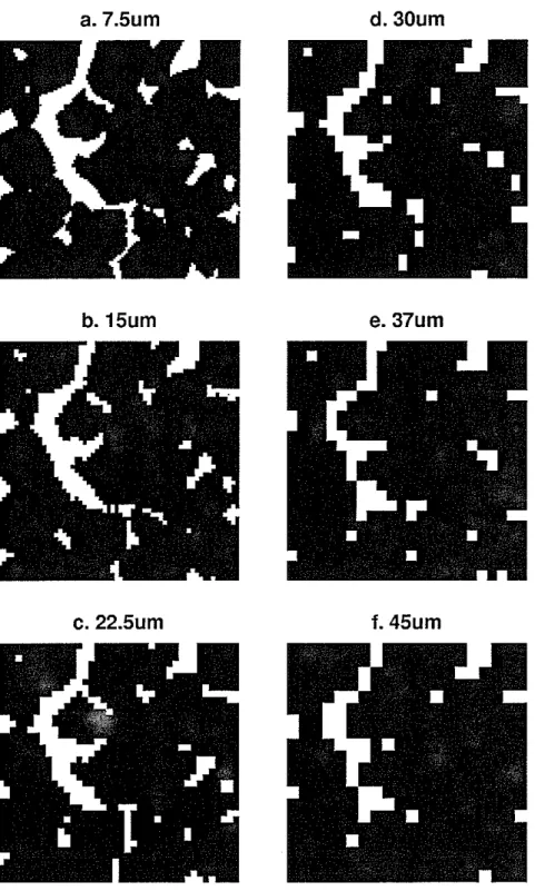
Looking at Figure 1, you can see that coarsening the resolution from 7.5 to 45 p.m
changes the quality of the image. At 7.5 p.m, the image has a complicated structure
that connects pores across the rock. Much of that structure is retained at 15 p.m, but
the connection across the sample is broken. As the resolution is coarsened further, the image captures only the largest pores and none of the small structure or connectors.
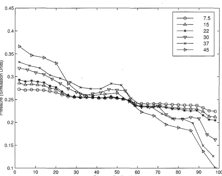
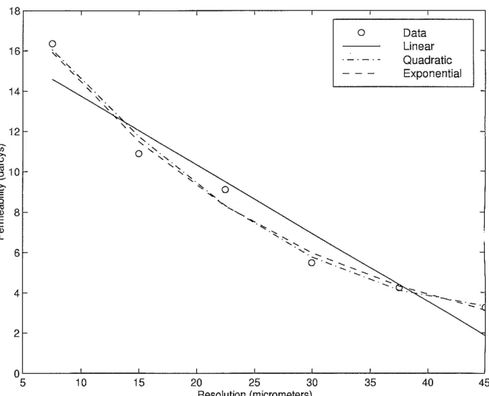
The loss of connection is evident in the change in pressure gradient across the sample at different resolutions. The pressure gradient increases as the size of the voxels increase as it becomes increasingly difficult for fluid to move through the rock. This relates to a decrease in permeability since it is inversely proportional to the pressure gradient (Figure 2). The permeabilities .calculated from the simulations range from 3.3 to 16.3 darcys, which are close to the laboratory measured permeability of 1.1 darcy. We try fitting the data with several types of curves (Figure 3). The relationship does not appear to be linear, but both the quadratic and the exponential are reasonable fits to the data. The permeability changes by a factor of five over the resolution range.
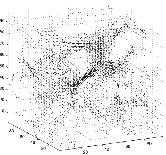
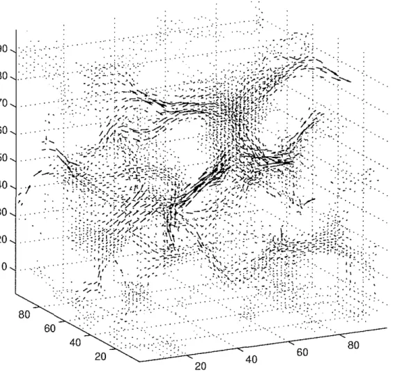
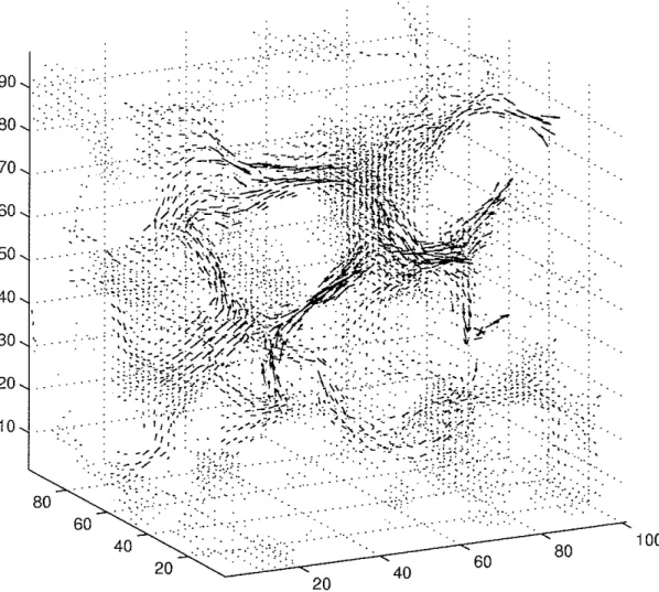
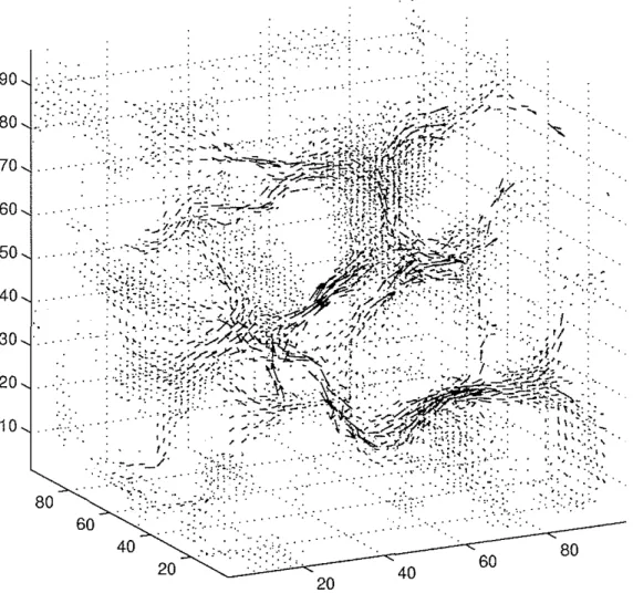
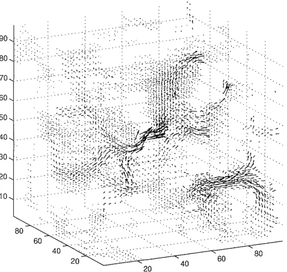
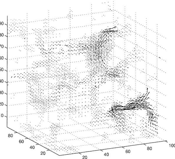
Velocity fields are plotted in Figures 4 through 9. The length of velocity vectors corresponds to equivalent magnitudes in all plots. The flow patterns are very similar until 30 m resolution. At that point, we see that the channel with the fastest flow in the center of the image is being constricted, and some flow is being diverted to the bottom front of the sample. Also, the two channels that feed the large pore at the top of the rock are narrowing. When we look at the 37.5 /-lm velocity field, we see that the secondary channel at the bottom of the rock has been disconnected and fluid is being forced again through the main channel in the center. Also, the path appears to have become more tortuous. At the top of the sample, the two channels have become disconnected from the large pore. The only preferential path is in the center of the sample. Looking at the 45 /-lm resolution image, the two channels at the top of the rock which fed the large pore have become one tortuous channel. The center channel has been cut off and a new path has been formed to the pore at the bottom corner of the rock.
DISCUSSION
Variations in image resolution seem to have a minor effect On permeability calculations from numerical simulation of fluid flow. The decrease in permeability is understandable when we look at the change in pore size as the resolution is changed in Figure 1. The pores become smaller and some of the connecting channels are lost. Also, SOme flow paths appear to become more tortuous as resolution decreases. Even so, the permeability change is relatively small since calculated permeability can vary due to subsampling of
the image by at least 2 orders of magnitude (Auzerias et al., 1996). Simulations were
run on subsets from the same image used in this study and it was found that for subsets of a similar size to ours, the permeability ranged from 0.1 to 10 darcys. Although we did not go to very coarse resolution (our lowest resolution being 45 /-lm), extrapolation of the permeability versus resolution curve suggests the effect would still be small even for coarser resolutions.
Unlike permeability, the velocity fields changed significantly from the finest to the coarsest resolution. The flow patterns changed due to changes in pore shape and con-nectivity as resolution varied. With coarsening, some small pores were eliminated, while
others that were clustered nearby became one large pore, resulting in new flow paths.
Itseems likely that the thresholding technique used to convert the image to boundary
conditions for the simulation will significantly influence how flow is distributed through-out the sample. The voxels in all images of porous media have numerical values from a continuous scale. For example, in NMR, voxels have values based on proton density, and this scale must be converted to a binary system where each voxel represents rock or pore. Ideally, the histogram of the voxel values would have a bimodal distribution representing pore space and grains, but this is rarely the case. Therefore, a decision must be made about where to place the cut-off value between pore and rock.
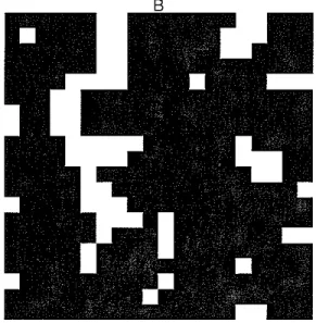
A simple experiment was carried out where the 7.5 p.m resolution image was coars-ened to 45 p.m but instead of using a threshold where half of the blocks needed to be pore in order for the new block to become pore, the threshold was only 1/4. The new image has much larger pores than the original image (Figure 10) and it is therefore not surprising that the calculated permeability is 19.2 darcys, which is not only much higher than the permeability originally calculated for the 45 p.m resolution image (3.3 darcys), but is also higher than the calculated permeability for the 7.5 p.m resolution image (16.3 darcys).
CONCLUSIONS
Resolution changes details of the pore structure in rock, but the pores responsible for
most of the flow are adequately captured. For resolutions ranging from 7.5 to 45 p.m,
the permeability only varied by a factor of five. Therefore, image resolution has little effect on permeability calculations, at least in this sample. However, if we imagine a rock that has a pore space distribution such that the smaller pores control flow (e.g., large pores connected by smaller throats), then the effect of resolution might be much larger. The image resolution did change some of the flow paths in the rock. Each voxel contains both rock and pore in reality, but for performing simulations each voxel must be designated either rock or pore. The way in which this image analysis is done, which in our case was a simple thresholding technique, impacts the dynamics of fluid flow since it affects whether smaller pores are left out or become larger, thereby changing the pore geometry. This effect is shown in a simple experiment where we change the threshold level and the permeability jumps from 3.3 to 19.3 darcys. Ultimately, we wish to obtain the best representative image, since it is impossible to precisely capture every detail of a complex porous rock. For understanding fluid dynamics in a porous medium, it seems that resolution, whether it is a few micrometers or tens of micrometers, is currently not a significant issue for the sample we investigated here.
ACKNOWLEDGMENTS
This work was supported by the Borehole Acoustics and Logging/Reservoir Delineation Consortia at the Massachusetts Institute of Technology.
REFERENCES
Auzerias, F., Dunsmuir, J., Ferreol, B., Martys, N., Olson, J., Ramakrishnan, R.,
Roth-man, D., and Schwartz, L., Transport in sandstone: A study on three dimensional
microtomography, Geophys. Res. Lett., 23, 705-708, 1996.
Edie, M.S., Fluid flow in porous media: NMR imaging and numerical simulation, M.S.
Thesis, MIT, 1999.
Kinney, J., Breunig., T., Starr, T., Haupt, D., Nichols, M., Stock, S., Butts, M., and
Saroyan, R., X-ray tomographic study of chemical vapor infiltration processing of
ceramic composites, Science, 260, 789-792, 1993.
Olson, J., Two-fluid flow in sedimentary rock: Complexity, transport and simulation,
Ph.D. Thesis, MIT, 1995.
Olson, J. and Rothman, D., Two-fluid flow in sedimentary rock: Simulation, transport,
and complexity, J. Fluid Mech., 341, 343-370, 1997.
Rothman, D. and Zaleski, S., Lattice-Gas Cellular Automata: Simple Models of Complex Hydrodynamics, Cambridge University Press, 1997.
a.7.5um
b.15um
c.22.5um
d.30um
e.37um
1.
45um
Figure 1: Cross section through sandstone showing pore space as the resolution is
changed from 7.5 to 45 fJ.m. Black areas are rock and white areas are pore space.
Notice the loss of small scale structure and connection across the sample as resolution is lowered.
0.451----,---,----,,---,---.---r--,---~2::==::::':==;l 0 7.5 8. 15 0.4
*
22 "i1 30 )( 37"
45 0.35 0.2 0.15 EJ 'c ::J § 0.3 ~ ::J E U5 ~ 0.25 ::J <J)~
0... 100 90 80 70 30 20 10 0.1 L -_ _L - _ - - - J L - _ - - - J_ _---J_ _---'_ _---'_ _--'-_ _--'-_ _--'-_---:o...Jo
Figure 2: Pressure versus distance across the rock showing change in pressure gradient as resolut ion is changed. The pressure gradient increases as the resolution is changed
from 7.5 to 45 J.!m. Permeability is calculated by taking.a linear, least-squares fit of
18
1
---,---,---.,---,---,---;==:=:::::====:::::===:=::;1
16 14o
"
"
"
\. ~.".
",
o
Data Linear Quadratic Exponential 12 6 4.-
~ -"'=:..."= . 2 45 40 35 20 25 30 Resolution (micrometers) 15 10 0 " - - - ' ' - - - ' - - - ' - - - ' - - - ' - - - ' - - - ' - - - ' 5Figure 3: Permeability versus distance across the rock showing decrease in permeability as resolution is coarsened. The trend does not appear to be linear, rather the decrease in permeability gets smaller as resolution increases.
90 80 70 60 50 40 30 20 '."...." ", . "..:'" ",". .~'." '.
.
...•~: 10 ... 80 -." . 60 40 20 '"':'.;:.:..' ..'...
,:.~ :'..'":.' ... '.
...; ,.:" ",::. :.",. .';. .:. ','Figure 4: 3D velocity field for simulation with 7.5 /-lm resolution image. The vector
length represents the magnitude of the velocity at that point in the rock. White areas are pores and areas with dots are low velocity zones in the rock. The axes show lattice units in all directions. There are two high velocity channels, one in the center of the image and one in the top, toward the left cor nero
". ',:... 90 80 70 60 50 40 30 ;!" .
.
,
" , "::'.
:;::.'.
.:~. '.'.
20...$,
;
;<:
s;..
~~~:...
80 20 40 60 20 ".
~ .:.~';.r;. .. : ....". :".'." : ,', . ' '. ,,-.?,'.: . :...: ! : :",.'..'.
.,,"..:-:·:i:'::· ..
:'.: . ,',." ; ~/...
:
..
"...,: 40 ;.., .": ",','" 60 80 10Figure 5: 3D velocity field for simulation with 15 "m resolution image. The vector length represents the magnitude of the velocity at that point in the rock. White areas are pores and areas with dots are low velocity zones in the rock. The axes show lattice
units in all directions. There is little change in the velocity field from the 7.5 "m
resolution image.
... ....
...
.,
" , ' I .: ."."" ....<>
'.:." ",'." ... ::.', >.: -:.':';:
.".; - ... ;y .. " .~. ".: .: .......
'. -, .···.·:;'~~,~~J;~"~mt~~'{?%+~
, . ' I •~t':' --.:... -:::::-/;--...;-.. • :.;.~~~n.ft!t\!;;". .1/'.
/ ' 1 / / , .• : :...;:: '" ':~;:II'~P~'.::-.. " ." -.' ".IJI..,f,;/.---=::..r..:--::/ ';I~ ....~~\ ,~' . :A~" - .
/1';7,·r,::-. """".' .' : :-V',~l ~\ .'.;;-,'/.' .' ... , . . . 'l'V~'''-' ,~.:::,,:::~"\>'
.. "
...
·.1
~t·~ ,~':"" ';%",;".~ :.:1;:C~~>:~~\l::;:>~;
. "~':.::":~:'.' . . " it;-"t:"':::',·..
~;:~~~i;.~~if-~
-...1 (j:-s.:"~: .\\\..
..
\::.::.~,~..
)/)1:;r"'}~::;A".,«,r," .. '.'
t:~ . >\:':':::;<>::;?~)J~/ . ' ';-:'.:-:"
' . /
'1,·- ..•..//~/-0,..(:~:.. ' -. -.,'. '..
..~~ ." . -. ' , : . . . : ,..:.. ~.:.~,. :.:.. 80 90 ...'. 80 70 60 50 40 30 20 10 60 40 20 20Figure 6: 3D velocity field for simulation with 22.5 /lm resolution image. The vector
length represents the magnitude of the velocity at that point in the rock. White areas are pores and areas with dots are low velocity zones in the rock. The axes show lattice units in all directions. The high velocity channel in the center seems to be more constricted
" ',. ::... .... :
,::
-,,". .:."."..:.":
" , ,..: . 40 60 80 80 ".' 70 60 50 40 30 20 .. 10 90Figure 7: 3D velocity field for simulation with 30 f.'m resolution image. The vector length represents the magnitude of the velocity at that point in the rock. White areas are pores and areas with dots are low velocity zones in the rock, The axes show lattice units in all directions. More flow is diverted to the channel at the bottom right corner than in the finer resolution images. Also, the two channels at the top left of the image which feed the big pore in the center, are narrower than in the finger resolution images.
.. ..
:
... . ...
"." .'-:.
-
...'-:
...~~- -.'..
...
.... ',' ....
~<:
~.,../<:. .~.
" . " ", ","',
. ~. .. . .. .. .... . .-'. ;~":": ' . .-.,' ..:..;;~ -:'...-~':.'.
.,.",',". : . 90 80 ','. 70 60 50 40 30 20 .-1, . 10 ,.", :... , "... .,.,' ~..:.. 80 . ' : ."; ~... 60 _',:.
.,
" ' ! • ".:. 40 ".:, '.,.... ... .~,' ... 20 '." ~ . , . ,. :'r . '.. .. .-. . F~'~;:
'.: 40 . ' 20 . > :: '-"~.
:.-. "', 60 80Figure 8: 3D velocity field for simulation with 37,5 fJ.m resolution image, The vector length represents the magnitude of the velocity at that point in the rock. White areas are pores and areas with dots are low velocity zones in the rock, The axes show lattice units in all directions. The channel in the bottom right COrner is wider than in the 30 fJ.m resolution image, and the velocity in the top left has decreased indicating that the connection has been disrupted to the main pore,
90
:::
:.:.:...
..: . , " ' - , .-;.: . .:-: . ,'.. 100 .., '..
80 .... ...:..
'.. 60 .'.".
":.:.;"';:.:::: 40 .~... 20 ' . " . ..
. .. . . . 20 40 ..,:. ....".:.: . '.:. 60 80 70 10 50 80 20 60 40 30Figure g: 3D velocity field for simulation with 45 I-lm resolution image. The vector length represents the magnitude of the velocity at that point in the rock. White areas are pores and areas with dots are low velocity zones in the rock. The axes show lattice units in all directions. Notice the flow at the top left has increased in velocity and there is only one channel where there used to be two at finer resolutions. Velocities are much smaller in the main center channel.
A B
Figure 10: Image of a cross section through the rock showing the effect of different thresholding levels. Notice that the pore size is much larger from the image with a threshold level of 0.5 (A) and a threshold level of 0.25 (B).