HAL Id: hal-01118700
https://hal.archives-ouvertes.fr/hal-01118700
Submitted on 19 Feb 2015
HAL is a multi-disciplinary open access archive for the deposit and dissemination of sci-entific research documents, whether they are pub-lished or not. The documents may come from
L’archive ouverte pluridisciplinaire HAL, est destinée au dépôt et à la diffusion de documents scientifiques de niveau recherche, publiés ou non, émanant des établissements d’enseignement et de
In-field crop row phenotyping from 3D modeling
performed using Structure from Motion
S. Jay, Gilles Rabatel, X. Hadoux, D. Moura, N. Gorretta
To cite this version:
S. Jay, Gilles Rabatel, X. Hadoux, D. Moura, N. Gorretta. In-field crop row phenotyping from 3D modeling performed using Structure from Motion. Computers and Electronics in Agriculture, Elsevier, 2015, 110, pp.70-77. �10.1016/j.compag.2014.09.021�. �hal-01118700�
Jay S., Rabatel G., Hadoux X., Moura D. & Gorretta N. (2015). In-field crop row phenotyping from 3D modeling performed using Structure from Motion. Computers and Electronics in Agriculture, 110, 70-77.
http://dx.doi.org/10.1016/j.compag.2014.09.021
Keywords: 3D modeling; Leaf area estimation; Phenotyping; Plant height estimation; Plant/background discrimination; Structure from Motion
In-field Crop Row Phenotyping from 3D Modeling
Performed Using Structure from Motion
Sylvain Jay*, Gilles Rabatel, Xavier Hadoux, Daniel Moura, Nathalie Gorretta
UMR ITAP, Irstea, 361, rue J.F. Breton, B.P. 5095, 34196 MONTPELLIER Cedex 5 *Corresponding author. Tel: +33 4 67 16 64 59. E-mail address: sylvain.jay@irstea.fr.
Abstract
This article presents a method for crop row structure characterization that is adapted to phenotyping-related issues. In the proposed method, a crop row 3D model is built and serves as a basis for retrieving plant struc-tural parameters. This model is computed using Structure from Motion with RGB images acquired by translating a single camera along the row. Then, to estimate plant height and leaf area, plant and background are discriminated by a robust method that uses both color and height information in order to handle low-contrasted regions. The 3D model is scaled and the plant surface is finally approximated using a triangular mesh.
The efficacy of our method was assessed with two data sets collected under outdoor conditions. We also evaluated its robustness against various plant structures, sensors, acquisition techniques and lighting conditions. The crop row 3D models were accurate and led to satisfactory height estimation results, since both the average error and reference measurement error were similar. Strong correlations and low errors were also obtained for leaf area estima-tion. Thanks to its ease of use, estimation accuracy and robustness under
outdoor conditions, our method provides an operational tool for phenotyping applications.
Keywords: Leaf area estimation, Phenotyping, Plant 3D modeling, Plant
height estimation, Plant/background discrimination, Structure from Motion.
1. Introduction
In a context of a greener and more competitive agriculture, the creation and selection of varieties consuming less water, nitrogen or even pesticides, have become a topic of major interest. Phenotyping methods are therefore needed in order to compare varieties and to relate genotypes to phenotypes. In particular, these methods aim at retrieving numerous parameters that characterize the crop row structure, such as plant height or leaf area. They must be non-destructive since these measurements have to be carried out all along the plant life. They must also be fast and automatic so that a maxi-mum of data may be processed with a minimaxi-mum of user interactions.
Plant structural parameters can be accurately retrieved from a three-dimensional (3D) model that can be computed in several ways. Active systems involving a light source have been used, e.g. with LiDAR (Rosell et al., 2009; Weiss and Biber, 2011) or the depth-imaging system Kinect Microsoft c (Ch´en´e et al., 2012). On the other hand, stereovision-based methods are passive and provide both the 3D structure estimate and color if an appropriate RGB camera is used. Because they can be implemented with commercial cameras, such methods have been widely used for agricultural applications (Ivanov et al., 1995; Andersen et al., 2005; Rovira-M´as et al., 2008).
Many authors have implemented stereovision to build plant 3D models using two view angles. These are often provided by two cameras that are separated by a fixed baseline distance and that need prior laboratory cali-bration. However, these methods do not always fulfill phenotyping-related constraints. For example, in their original implementation, some of them can-not be easily implemented in the field (Shrestha et al., 2003) or are dedicated to a single variety and thus not applicable for varietal selection (He et al., 2002). Only a few methods can be used for such applications. For example, Kise and Zhang (2008) have developed a system using one tractor-mounted stereocamera for 3D crop row structure mapping. Their system estimates the height and position of crop rows in order to reliably guide the tractor. Leemans et al. (2013) have also used images acquired by a stereocamera for leaf area index retrieval in wheat crops. Recently, Lati et al. (2013) have developed a novel approach for the estimation of plant height, leaf cover area and biomass volume, which can even handle occluded areas to some extent (i.e., overlapping leaves).
On the other hand, using Structure from Motion (SfM) to retrieve the crop row 3D structure is easier than using stereovision with several cameras. In-deed, as explained in Section 2.1, SfM is implemented with only a single camera acquiring images while moving along the row. Furthermore, since camera intrinsic parameters are automatically estimated during the recon-struction process, SfM does not need any prior calibration and is therefore a convenient tool for in-field phenotyping applications. It has been used for plant 3D modeling (Santos and de Oliveira, 2012), but its potential for plant
structural parameter retrieval has not been explored much yet.
Retrieving plant structural parameters from crop row 3D models often necessitates to discriminate plant from background. Usual discrimination methods are color-based and involve thresholding a vegetation index map computed from RGB bands. Many of these vegetation indices have been re-viewed by Meyer and Neto (2008). One of the most widely used is the Excess Green Index (ExG) first introduced by Woebbecke et al. (1995). However, even though this index is normalized and thus insensitive to the light source intensity and leaf inclination (G´ee et al., 2008), it is affected by shadows. Indeed, in shaded areas, the light mainly originates from multiple scattering caused by the nearby environment (Vigneau, 2010). Therefore, the result-ing light variations cannot be accurately modeled with a sresult-ingle multiplicative factor. Recently, Lati et al. (2013) have discriminated plant from background in a more appropriate two-dimensional color space also based on RGB bands. They have used a hue-invariant transformation that takes into account spec-tral properties of natural light. However, this method is not automatic be-cause for each situation, several parameters that depend on the sensor and contrast between plant and background have to be set beforehand. In ad-dition, like other color-based discrimination methods, this approach fails if this contrast is low.
In this study, we propose a 3D modeling based method to character-ize crop rows under outdoor conditions, i.e., to retrieve their structure, plant height and leaf area. Phenotyping-related needs (non-destructive, automatic, fast) are considered, and special attention is given to the robustness against
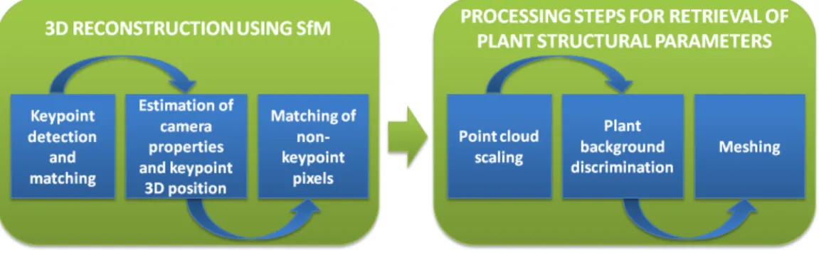
Figure 1: Framework of the proposed method.
heterogeneous lighting and low-contrasted regions. First, we perform 3D reconstruction using SfM and second, we retrieve the plant structural pa-rameters from the crop row 3D model.
This paper is organized as follows. Section 2 presents the proposed method. The data sets and implementation details are described in Section 3. Sec-tion 4 shows the results of 3D reconstrucSec-tion, discriminaSec-tion and retrieval of plant structural parameters. Lastly, Section 5 draws conclusions and provides some guidelines for further work.
2. Proposed method
The framework of the proposed method is illustrated in Fig. 1. The first part deals with the 3D reconstruction performed using SfM, while in the second part, various processing steps are applied to the 3D model in order to retrieve the plant structural parameters. Both parts are described in the two following sections.
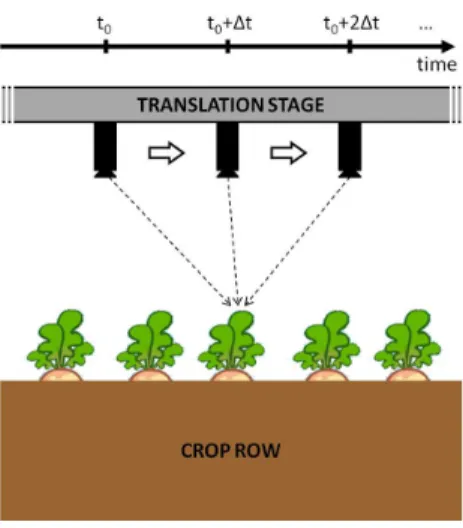
Figure 2: Example of experimental setup used to implement Structure from Motion. The camera is translated along the crop row so as to image every point from various view angles (represented by dashed arrows).
2.1. 3D reconstruction using Structure from Motion
Stereovision enables an object 3D structure to be retrieved from 2D im-ages acquired from different view angles. Using SfM, the view angles are obtained by moving a single camera around the object of interest. The mo-tion is either free or forced by a translamo-tion stage as illustrated in Fig. 2. In this latter case, the camera is translated at a given speed and acquires an image every time interval ∆t. If ∆t is small enough, images are overlapping so every point is seen from various view angles. Techniques based on ray intersection then allows us to retrieve the 3D position of such a point as well as the associated camera positions and orientations (Kraus, 2007).
In this method, we implemented SfM with Micmac (Ign, 2013), a digital surface model freeware developed by the National Institute of Geographic
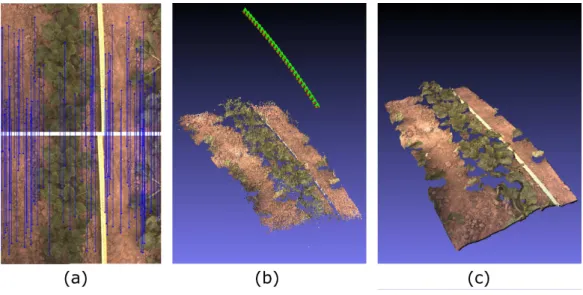
and Forest Information. In the following, we briefly describe the three usual main steps of SfM and their Micmac implementation. For more information, the reader can refer to the associated documentation (Ign, 2013). These steps are also illustrated on a real example in Fig. 3.
As shown in Fig. 3a, the first step consists in identifying points that are seen in several images. For this purpose, Micmac implements the Scale-invariant feature transform (SIFT) (Lowe, 1999), which has been designed to provide feature descriptors that are invariant to scale, rotation, translation and expo-sure. Then, basically, for every couple of images, a feature point in the first image is matched with the most similar feature point in the second image (in terms of Euclidean distance). This step thus allows many points of the scene to be detected in different images.
In the second step, the 3D position of every matched feature point is es-timated together with the camera internal calibration and its position and orientation for every image. To do so, Micmac implements an iterative pro-cess in which, at the iteration N, ray intersection and matched feature points are used to orientate the Nth
image with respect to the (N −1) previous ones (the first image being arbitrarily orientated). A distortion model (usually ra-dial) with several degrees of freedom (one for the focal length, two for the position of the principal point, and others for distortion coefficients) is used to estimate the camera internal calibration from the image set. At the end of each iteration, a bundle adjustment (Hartley and Zisserman, 2004) is also performed in order to limit error accumulation. A sparse point cloud de-scribing the positions of feature points is therefore obtained as illustrated in Fig. 3b.
Figure 3: Main steps of 3D reconstruction: (a) Feature point detection and matching for a pair of images; (b) Sparse 3D point cloud (camera positions and orientations in green); (c) Dense 3D point cloud.
Lastly, in the third step, the estimated camera orientations and positions are used to retrieve the 3D positions of non feature point pixels, thus generat-ing a dense point cloud. In Micmac, a matchgenerat-ing process usgenerat-ing normalized cross-correlation is implemented. For a given pair of overlapping images, a pixel in the first image is associated with the pixel that is on the epipolar line in the second image and that maximizes the cross-correlation criterion. This operation is repeated for every couple of images so that the estimated position of a given point be less noise-sensitive. The computed dense point cloud is shown in Fig. 3c.
2.2. Retrieval of plant structural parameters
Once the crop row structure has been estimated, the 3D model has to be processed in order to extract plant structural parameters.
First, we set the point cloud to an appropriate scale in order to get height and area values in SI units (resp. cm and cm2).
The following step is to discriminate plant-related pixels from background-related pixels. Because the process may be applied to a large amount of data, this discrimination has to be automatic. Moreover, various backgrounds may be found (soil, sand, grass, wood, etc) so we use both height (H) and color within a clustering algorithm to improve the plant/background discrimina-tion, the underlying hypothesis being that the plants of interest are greener and higher than the background.
In this study, both the vegetation index ExG and the two variables intro-duced by Lati et al. (2013) were compared. ExG is derived from the RGB values R, G and B as follows:
ExG = 2G − R − B
R + G + B . (1)
The variables used by Lati et al. (2013) are based on the CIE xyY color space that is obtained from the RGB space. Under various assumptions including Planckian illumination (natural light), using log-chromaticity allows the illu-mination color variations to be easily identified. Lati et al. (2013) have used such information through the two variables log (x/y) and log (Y /y) derived from the xyY values.
With ExG, pixels belonging to the plant class (resp. background class) have high (resp. low) ExG values, which makes their identification more straight-forward. Using the space spanned by the variables of Lati et al. (2013) may allow us to better address misclassification occurring under natural light. Once both classes have been discriminated, plant height is estimated by com-puting the plant highest height minus the mean ground height. The latter is
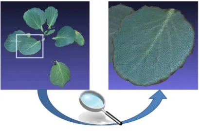
Figure 4: Reconstructed leaf surface.
the mean height of background-related pixels located in a local neighborhood centered on the plant.
Finally, a triangular meshing of the plant point cloud is performed and leaf area is estimated by summing every triangle area. Fig. 4 illustrates this last step by showing an example of reconstructed leaf surface.
3. Experiments
3.1. Data
Two data sets were created in order to assess the performance and ro-bustness of our method regarding sensors, acquisition techniques, lighting conditions and crop row structures.
3.1.1. Image acquisition
For the first data set, we used a digital single-lens reflex camera (Canon 500D) to acquire 1176×784 pixel images. Four plant species having
differ-ent structures were imaged: sunflowers (Helianthus annuus), Savoy cabbages (Brassica oleracea var. sabauda), cauliflowers (Brassica oleracea var.
botry-tis) and Brussels sprouts (Brassica oleracea var. gemmifera). The camera
was orientated towards nadir and images were acquired approximately every 10 cm by manually moving the camera at about 1 m above the ground level (depending on plant height).
The second data set was collected in sugar beet (Beta Vulgaris L.) fields in Vimy (northern France) within the framework of AKER project1. Two sugar
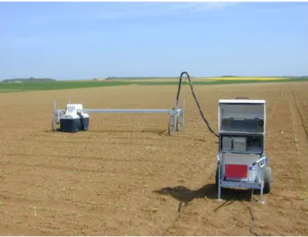
beet varieties (Eleonora and Python) subjected to four different nitrogen ap-plications were imaged at two growth stages using the Becam phenotyping platform2 (Benet and Humbert, 2009) presented in Fig. 5. A 6 mm lens was
mounted on a digital CCD camera (Teledyne Dalsa Genie C1024) acquiring 1024×768 pixel images (note that the sensor quality was lower than for the first data set). The camera was set up on the translation stage, orientated towards nadir at 1.20 m above the ground level and acquired images every 4 cm along the crop row. With this setup, every point of the scene was im-aged from a dozen different view angles.
For both data sets, before image acquisition, a measuring tape was placed into the scene in order to scale the spatial unit of the 3D model.
1AKER is a project funded by the French National Research Agency and partly devoted
to sugar beet phenotyping
2The Becam phenotyping platform was developed by Irstea for plant counting and
Figure 5: Becam phenotyping platform.
Table 1: Height (H) and leaf area (LA) ranges for the two data sets (min - max).
Data set 1 Data set 2
Sunflower Savoy cabbage Cauliflower Brussels sprout Sugar beet H (cm) 15 - 65 10 - 17 19.5 - 22.5 11.5 - 17.5 × LA (cm2) 27 - 1201 99 - 331 360 - 538 80 - 573 378 - 622
3.1.2. Reference measurements
Plant height was measured manually from the mean ground level to the highest point of the plant. To measure leaf area, limbs were harvested, placed on blank sheets and flattened with a pane of glass. They were then scanned and after extraction of leaf-related pixels by image processing, their area in cm2 was estimated using the calibrated pixel size.
In the second data set, only one mean measurement of leaf area (carried out on four to six plants) was available for each crop row.
The ranges of height and leaf area for the two data sets are reported in Tab. 1. Note that height was not measured for the second data set.
3.2. Implementation
In order to fulfill phenotyping-related constraints, we implemented Mic-mac in such a way that the proposed method was automatic and reasonably fast (a few dozen minutes using a personal computer). First, the option ”ground geometry” was selected because it did not necessitate any user in-teraction. This option is well adapted for the reconstruction of many plant species, especially in early growth stages, however it does not allow occluded regions to be handled. Second, the time needed for feature point detection was shortened by considering the crop row linear structure. For the two data sets, most points of the study zones were only seen in a dozen successive images so the detection process was restricted to these images.
Concerning structural parameter retrieval, the point cloud was first scaled using a measuring tape placed in the study zone. Note that for the Becam setup, images were acquired using a known constant baseline length. There-fore, the scaling parameter could potentially be automatically retrieved by fitting the mean baseline length estimated from the 3D model (in arbitrary unit), to the actual length (in SI unit).
Discrimination was performed by clustering pixels around two class centers using the k-means (KM) algorithm (Lloyd, 1982), and assigning the label ”plant” to the class containing the greenest and highest pixels.
The plant surface was finally approximated using the ball-pivoting algorithm (Bernardini et al., 1999) implemented in Meshlab (Meshlab, 2014).
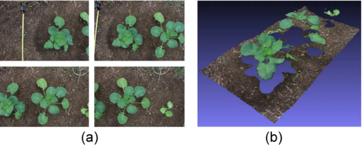
Figure 6: Brussels sprout row reconstruction performed with 18 images. (a) RGB images; (b) 3D model.
3.3. Method performance assessment
Discrimination methods were compared using the overall accuracy (OA), which is the percentage of well classified pixels.
In order to assess height and leaf area estimation, we used the well-known coefficient of determination (R2) and root mean square error (RMSE). We
also indicated the mean absolute error (MAE) because it has proven to be a more reliable measure of average error than RMSE (Willmott and Matsuura, 2005), especially when comparing estimation results obtained with samples of different size.
We compared the estimated leaf area with the leaf cover area, which is a simple measure of leaf area defined by the point cloud projected area onto the background plane.
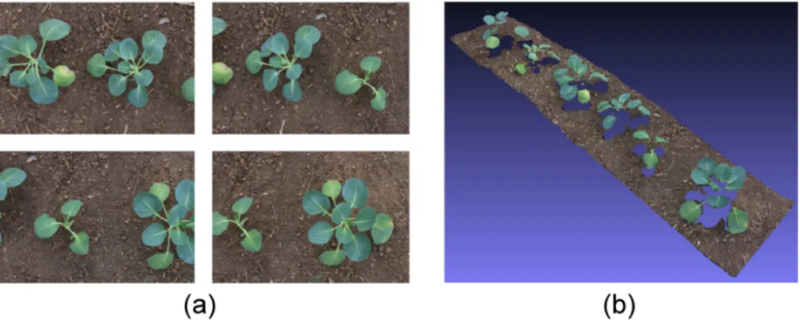
Figure 7: Savoy cabbage row reconstruction performed with 38 images. (a) RGB images; (b) 3D model.
4. Results and discussions
4.1. 3D reconstruction
Three 3D models obtained with the first data set are presented in Fig. 6 (Brussels sprouts), Fig. 7 (Savoy cabbages) and Fig. 8 (sunflowers). The 3D model of sugar beet row obtained from the second data set is shown in Fig. 3c. In every case, the estimated leaf orientations and background shape were accurate. Every plant was well reconstructed even though the acquisition techniques and sensors were different within the two data sets.
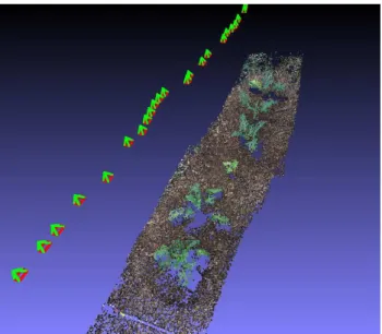
For the first data set, the translation motion was performed manually, by moving the camera horizontally above the ground level. As a result, the camera altitude, view angle and baseline distance between two successive positions were differing from one image to the other (see Fig. 9). However, this did not affect the reconstruction process, which proves that the method is easy to implement because it does not need a specific imaging setup. For the second data set, the camera was forced to move along the translation
Figure 8: Sunflower row reconstruction performed with 16 images. (a) RGB images; (b) 3D model.
Figure 9: Sparse point cloud computed with images acquired from varying orientations and positions.
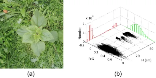
Figure 10: Example of low-contrasted scene. (a) Original RGB image; (b) Distribution of ExG and H.
stage but the sensor quality was lower than for the first data set. However, an accurate 3D model was obtained as well, thus showing the efficacy of Micmac even when using poorer sensors.
The reconstruction was performed using a personal computer with a 3.60 GHz processor and 4 GB of RAM. Overall processing times per image ranged from 30 to 60 seconds, depending on the crop row structure complexity and the number of images. Even though these processing times are longer than those obtained with a stereocamera (especially because the feature point detection is performed for several couples of images instead of one couple of left and right images), they are quite acceptable for such applications.
4.2. Plant/background discrimination
The interest of using height for discrimination (especially in low-contrasted areas) is demonstrated in Fig. 10. In the RGB image shown in Fig. 10a, the sunflower and background have similar ExG values ranging from 0 to 0.8, so
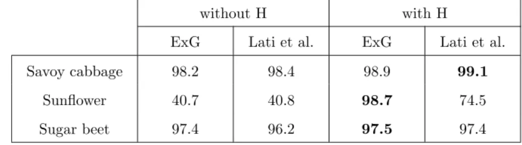
Table 2: Comparison of discrimination overall accuracy obtained without and with height. Color information is given either with ExG or the two variables of Lati et al. (2013). For each of the three considered crop structures, the best results are in bold.
without H with H
ExG Lati et al. ExG Lati et al.
Savoy cabbage 98.2 98.4 98.9 99.1
Sunflower 40.7 40.8 98.7 74.5
Sugar beet 97.4 96.2 97.5 97.4
the overall ExG distribution contains only one mode (see the green histogram in Fig. 10b). Consequently, color is not relevant enough to discriminate plant and background classes. On the other hand, the red histogram displaying the height distribution contains at least two distinct modes (one for the back-ground and several for the plant), which shows that height information can remove the ambiguity occurring when using color only.
More detailed discrimination results are provided in Table 2. KM cluster-ing methods based on color with and without height are compared, color information being given by either ExG or the two variables introduced by Lati et al. (2013). We considered images from the two data sets, i.e, Savoy cabbage and sunflower for the first data set, and sugar beet for the second data set.
We observe that height information is very important when the contrast be-tween plant and background is low (i.e., for sunflower), since the maximum overall accuracy increased from 40.8% to 98.7% when H was used. We also note a positive influence when the contrast is high because in such cases (i.e., for Savoy cabbage and sugar beet), the best overall accuracy was still
Figure 11: Height estimation results obtained with the first data set.
obtained using height information.
On average, for the two data sets, the best results were obtained combining H and ExG. Using both variables also addresses one of the problems raised by Lati et al. (2013), i.e., misclassification occurring under natural lighting. Indeed, our approach well discriminates such regions because height infor-mation somewhat compensates these heterogeneous lighting conditions. Therefore, we used both ExG and H before retrieving height and leaf area.
4.3. Plant height estimation
Fig. 11 shows the height estimation results obtained with the first data set. For every species, estimated heights are plotted against actual heights. We obtained a strong linear correlation and low average errors between esti-mated and actual values (R2 = 0.99, RMSE = 1.1 cm, MAE = 0.85 cm). The
RMSE was similar to the measurement error caused by rough backgrounds and moving leaves, which demonstrates that the crop row 3D models provide
Figure 12: Height map of a Savoy cabbage row (in cm).
Figure 13: Height map of a sunflower row (in cm).
extremely accurate estimates of plant height. Furthermore, the proposed method obtained high R2 and low RMSE and MAE for every species, thus
proving that the method can handle various crop structures.
The good estimation accuracy observed in Fig. 11 indicates that realistic height maps of crop rows can be obtained as illustrated in Fig. 12 and Fig. 13 for Savoy cabbage and sunflower respectively. Highest leaves of Savoy cab-bages were situated in the centers of the plants, whereas the lowest leaves were situated on the borders. The specific structure of sunflower, i.e., flat leaves at different heights, was also well retrieved. One can also note that the resolution and accuracy of these maps also allow a good estimation of
Figure 14: Leaf area estimation results obtained with the first data set.
local leaf inclination in the whole plants.
4.4. Leaf area estimation
Both data sets were used to assess the leaf area estimation process. For the first data set, in Fig. 14, estimated leaf areas are plotted against actual leaf areas for every species. We obtained a strong linear correlation and low average errors between estimated and actual values (R2 = 0.94,
RMSE = 85 cm2, MAE = 59 cm2), which shows the potential of our method
for leaf area estimation under outdoor conditions. In addition, the estimation results were good for every single species since the relative MAE were 12% for sunflower and Brussels sprout, 16% for cauliflower, and 21% for Savoy cabbage. These results prove that the performance remained stable for the considered plant structures.
The leaf area estimation results obtained with the second data set are shown in Fig. 15. For each row, the actual mean value is compared with the mean
Figure 15: Estimated leaf areas obtained with the second data set. The errors bars are the sample standards deviations computed from four to six plants.
value estimated with the proposed method, and the estimated mean leaf cover area. Sample means and standard deviations (shown with error bars) were computed from four to six plants. The estimated mean leaf areas were close to the actual mean leaf areas since the RMSE and MAE computed with these mean values were 66 cm2 and 45 cm2 respectively (i.e., 13% and 9%
resp.). The actual mean leaf areas were in the intervals specified by sample standard deviations except for row 6. In this latter case, the results were less accurate because of overlapping leaves that were not handled by our method. We also see that leaf cover area did not provide a good estimate of leaf area in this case. High leaf inclination was observed for such developed plants, which made projected leaf area and actual leaf area very different.
5. Conclusions and further work
This study presents a method to retrieve crop row structure and struc-tural parameters, i.e., plant height and leaf area. It has been designed in order to fulfill phenotyping-related needs to some extent (non-destructive, automatic, robust, fast).
The crop row 3D structure is retrieved using SfM so the camera calibra-tion parameters are automatically estimated from the data. A 3D model is computed from 2D images acquired by a single moving camera, and various processing steps are then implemented before retrieving structural param-eters. First, the point cloud is scaled to get measurements in centimparam-eters. Then, plants and background are discriminated with a robust and automatic method that uses both height and color information in order to handle low-contrasted scenes. A triangular meshing is finally performed to approximate the leaf surface.
This method was tested on two data sets collected under outdoor conditions. Its robustness was proven against various crop structures, acquisition tech-niques, sensors and lighting conditions. For the five studied plant species, accurate crop row 3D models were computed. The proposed discrimina-tion approach led to better results than those obtained with color-based approaches. Finally, plant height and leaf area were well estimated since high correlations and low average errors were obtained between estimated and actual values.
However, the method does not consider occluded leaves and further investi-gation is needed to retrieve leaf area for such plant structures. Though we did not encounter wind-related problems, it is also a major obstacle when
using SfM in field instead of a stereocamera. The plants may be not in the same position from one image to the other, which would lead to poorer re-construction results. This problem could be overcome by using two or more cameras acquiring simultaneously images from different view angles.
Acknowledgments
This study was funded by the French National Research Agency, within the program ”Investissements d’avenir” with the reference ANR-11-BTBR-0007 (AKER project). We are grateful to the French Sugar Beet Technical Institute (ITB), which made the Becam platform available to us and carried out leaf area measurements within AKER project.
References
Andersen, H.J., Reng, L., Kirk, K., 2005. Geometric plant properties by relaxed stereo vision using simulated annealing. Computers and Electronics in Agriculture 49, 219–232.
Benet, B., Humbert, T., 2009. R´ealisation du systeme Becam portique pour l’acquisition d’images sur deux raies de betteraves. Technical Report. Cemagref.
Bernardini, F., Mittleman, J., Rushmeier, H., Silva, C., Taubin, G., 1999. The ball-pivoting algorithm for surface reconstruction. IEEE Transactions on Visualization and Computer Graphics 5, 349–359.
Ch´en´e, Y., Rousseau, D., Lucidarme, P., Bertheloot, J., Caffier, V., Morel, P., Belin, E., Chapeau-Blondeau, F., 2012. On the use of depth camera for
3D phenotyping of entire plants. Computers and Electronics in Agriculture 82, 122–127.
G´ee, C., Bossu, J., Jones, G., Truchetet, F., 2008. Crop/weed discrimination in perspective agronomic images. Computers and Electronics in Agricul-ture 60, 49–59.
Hartley, R.I., Zisserman, A., 2004. Multiple View Geometry in Computer Vision. Second ed., Cambridge University Press, isbn: 0521540518.
He, D., Hirafuji, M., Kozai, T., 2002. Growth prediction of a transplant population using artificial neural networks combined with image analysis, in: Third Asian Conference for Information Technology in Agriculture (AFITA 2002), Beijing, China, pp. 266–271.
Ign, 2013. Micmac documentation. Retrieved July 24, 2014, from http://logiciels.ign.fr/?Micmac.
Ivanov, N., Boissard, P., Chapron, M., Andrieu, B., 1995. Computer stereo plotting for 3-D reconstruction of a maize canopy. Agricultural and Forest Meteorology 75, 85 – 102.
Kise, M., Zhang, Q., 2008. Development of a stereovision sensing system for 3D crop row structure mapping and tractor guidance. Biosystems Engi-neering 101, 191 – 198.
Kraus, K., 2007. Photogrammetry: geometry from images and laser scans. de Gruyter ed., Walter de Gruyter & Co, isbn: 9783110190076.
Lati, R.N., Filin, S., Eizenberg, H., 2013. Estimating plant growth param-eters using an energy minimization-based stereovision model. Computers and Electronics in Agriculture 98, 260–271.
Leemans, V., Dumont, B., Destain, M., 2013. Assessment of plant leaf area measurement by using stereo-vision, in: 2013 International Conference on 3D Imaging (IC3D), Liege, Belgium, pp. 1–5.
Lloyd, S., 1982. Least square quantization in PCM. IEEE Transactions on Information Theory 28, 129–137.
Lowe, D.G., 1999. Object recognition from local scale-invariant features, in: Proceedings of the Seventh IEEE International Conference on Computer Vision, Kerkyra, Greece, pp. 1150–1157.
Meshlab, 2014. Retrieved July 24, 2014, from http://meshlab.sourceforge.net/.
Meyer, G., Neto, J., 2008. Verification of color vegetation indices for auto-mated crop imaging applications. Computers and Electronics in Agricul-ture 63, 282–293.
Rosell, J.R., Llorens, J., Sanz, R., Arn´o, J., Ribes-Dasi, M., Masip, J., Es-col`a, A., Camp, F., Solanelles, F., Gr`acia, F., Gil, E., Val, L., Planas, S., Palac´ın, J., 2009. Obtaining the three-dimensional structure of tree orchards from remote 2D terrestrial LIDAR scanning. Agricultural and Forest Meteorology 149, 1505 – 1515.
terrain maps for precision agriculture. Computers and Electronics in Agri-culture 60, 133 – 143.
Santos, T.T., de Oliveira, A.A., 2012. Image-based 3D digitizing for plant architecture analysis and phenotyping, in: Workshop on Industry Applica-tions (WGARI) in SIBGRAPI 2012 (XXV Conference on Graphics, Pat-terns and Images), Ouro Preto, MG, Brazil, pp. 21–28.
Shrestha, D., Steward, B., Kaspar, T., 2003. Determination of early stage corn plant height using stereo-vision, in: 6th International Conference on Precision Agriculture and Other Precision Resources Management, Min-neapolis, MN, USA, pp. 1382–1394.
Vigneau, N., 2010. Potentiel de l’imagerie hyperspectrale de proximit´e comme outil de ph´enotypage : application a la concentration en azote du bl´e. Ph.D. thesis. Montpellier SugAgro, France.
Weiss, U., Biber, P., 2011. Plant detection and mapping for agricultural robots using a 3D LIDAR sensor. Robotics and Autonomous Systems 59, 265 – 273.
Willmott, C.J., Matsuura, K., 2005. Advantages of the mean absolute error (MAE) over the root mean square error (RMSE) in assessing average model performance. Climate Research 30, 79–82.
Woebbecke, D.M., Meyer, G.E., Bargen, K.V., Mortensen, D.A., 1995. Color indices for weed identification under various soil, residue, and lighting con-ditions. Transactions of the ASAE 38, 259–269.