Distributed visibility servers

(1)

Distributed Visibility Servers

by

Eric A. Brittain

Submitted to the Department of Electrical Engineering and Computer Science in Partial Fulfillment of the Requirements for the Degree of

MASTER OF SCIENCE

IN ELECTRICAL ENGINEERING AND COMPUTER SCIENCE AT THE

MASSACHUSETTS INSTITUTE OF TECHNOLOGY

May 24, 2001

The author hereby grants to M.I.T. permission to reproduce and distribute publicly paper and electronic copies of this thesis and to grant others the right to do so.

Author

Department of iectrical Engineering and Computer Science May 24, 2001

Certified by

Seth J. Teller Associate Professor of Computer Science and Engineering Thesis Supervisor

Accepted by

'rthur C. Smith

Chairman, Department Committee on Graduate Theses

BARKER MASSACHUSETTS INSTITUTt

OF TECHNOLOGY

JUL 11 2001 LIBRARIES

(2)

Distributed Visibility Servers

by

Eric Brittain

Submitted to the

Department of Electrical Engineering and Computer Science on May 24, 2001

In partial fulfillment of the requirements for the degrees of Master of Science in Electrical Engineering and Computer Science

Abstract

This thesis describes techniques for computing conservative visibility exploiting viewpoint prediction, spatial coherence and remote visibility servers to increase the rendering performance of a walkthrough client. Identifying visible (or partially visible) geometry from an instantaneous viewpoint of a 3-D computer graphics model in real-time is an important problem in interactive computer graphics. Since rendering is an expensive process (due to transformations, lighting and scan-conversion), successfully identifying the exact set of visible geometry before rendering increases the frame-rate of real-time applications. However, computing this exact set is computationally intensive and prohibitive in real-time for large models.

For many densely occluded environments that contain a small number of large occluding objects (such as buildings, billboards and houses), efficient conservative visibility algorithms have been developed to identify a set of occluded objects in real-time. These algorithms are conservative since they do not identify the exact set of occluded geometry. While visibility algorithms that identify occluded geometry are useful in increasing the frame-rate of interactive applications, previous techniques have not attempted to utilize a set of workstations connected via a local area network as an external compute resource. We demonstrated a configuration with one local viewer and two remote servers.

Thesis Supervisor: Seth Teller

(3)

Acknowledgements

First, I would like to thank God for giving me the strength to complete this thesis.

Without His love and support, this work would not be possible. I would like to extend

special thanks to my advisor, Seth Teller, who has supported me from the very first day I

arrived at MIT. I would also like to thank the members of the Computer Graphics Group

for their support.

I would like to thank my family for loving and supporting me while I am away at

school at MIT. Without their support, I would not have been able to accomplish this task.

I would like to send a special thank you to all my friends who supported me during this

(4)

List of Figures

Figure 1 A Traditional Rendering Pipeline ... 17

Figure 2 V iew Frustum Culling ... 17

Figure 3 O cclusion Culling ... 18

Figure 4 O cclusion in 2D ... 19

Figure 5 k-d Tree ... 21

Figure 6 Region-to-Region V isibility ... 25

Figure 7 2D V isibility Cell D ecom position ... 27

Figure 8 V isibility Tree ... 28

Figure 9 D raw ing tim e...32

Figure 10 O cclusion culling tim e ... 33

Figure 11 O verall Fram e rate... 35

Figure 12 O ccluder Selection O ption... 44

Figure 13 O ccluder Selection Trackball V iew ... 45

Figure 14 Client Rendering Perform ance W indow ... 48

Figure 15 Client Trackball W indow s ... 49

(8)

List of Tables

Table 1 D escription of Server O ptions... 46 Table 2 Description of Client Options ... 47

(9)

List of Equations

(10)

Chapter 1: Introduction

1.1 Overview

This section of the thesis provides an overview of the visibility problem and the

approach that was taken to accelerate its computation. Visibility determination is the

problem of identifying graphical primitives in a scene that is visibility from a synthetic

camera. In real-time 3D walkthrough applications1, computing the exact set of visible primitives in a scene that contains several million graphical primitives is prohibitive. The

Z-Buffer [7] visibility algorithm produces a final output image by rendering all primitives

into a special buffer (known as Z-buffer) and overwriting previously written pixels in the

buffer that were further away from the camera (depth comparisons). Given a scene with

n primitives, each pixel on the screen has the capability of being "overdrawn" n times. If

the scene contains several million primitives and has high depth complexity, the Z-Buffer

algorithm is too slow to be used in a real-time application.

In an attempt to render very large scenes in real time, many computer graphics

researchers have resulted to computing conservative visibility to augment the widely used

Z-Buffer algorithm. A visibility algorithm is said to be conservative if it never

(11)

incorrectly identifies a visible primitive as invisible. This is possible because the

Z-Buffer algorithm is typically the last stage of the visibility process and will resolve all

final visibility relationships. The goal of conservative algorithms is to find a small

superset of the visible set of primitives and render them using the graphics pipeline. In

the worst case, the conservative algorithm would return all primitives in the scene.

However, it is the goal of these conservative algorithms to return a set of primitives much

smaller than the complete set of primitives and thus decrease the rendering time.

Up until this point, most visibility algorithms have been designed to work on

single processor or multiple processor parallel machines. Our search into the literature

did not reveal any work seeking to compute visibility by a cluster of workstations. In this

thesis, we discuss methodologies and results of computing visibility on a distributed

cluster of workstations in hopes of computing visibility faster than computing it using a

single processor system.

1.2 Motivation

In order to render 3D scenes for an interactive computer graphics application,

several steps (or stages) are usually performed in series (or in parallel). First, a sequence

of transformations is established to dictate how the objects in the scene will appear on the

screen (known as viewing and model transformations). Secondly, each object in the

scene is tested against some visibility criterion to determine if it will appear in the output

(12)

next stage; otherwise it is removed from the rendering pipeline. Finally, each object is

rendered using the Z-Buffer algorithm and finally displayed on the screen.

Most real-time computer graphics systems that compute visibility do so by

performing all needed visibility calculations on the same machine that is rendering the

scene. Typically, each object is tested in real-time and determined to be either potentially

visible or invisible. The work in this thesis seeks to decouple the visibility computation

from the normal real-time rendering pipeline.

Motivated by the University of California at Berkeley's Network of Workstations

project (NOW) [4], we sought to develop a distributed algorithm that could use multiple

workstations connected via a Local Area Network (LAN) to accelerate the visibility

calculations. The goal of the Berkeley NOW system was to provide software and

hardware support for using a NOW as a distributed supercomputer on a building-wide

scale. While the Berkeley system used advanced switching network to achieve high

performance communications, we are using off-the-shelf Ethernet components for our

system. The rationale for this decision was that since single CPU networked systems are

cheaper than shared memory computers, it would be interesting to see if we could build a

system out of these cheaper CPUs and achieve comparable performance. In building

such a system, we had to change the existing visibility algorithms to work in this new

(13)

1.3 Related Work

Several papers have been published on the topic of computing visibility. In the

context of computing exact visibility [16] and [17] describes the output image in terms of

visible polygon fragments. While these algorithms can find the exact set of visible

polygon fragments, they tend to be complex and difficult to use in interactive

applications. The Z-buffer algorithm [7] is an exact algorithm that resolves visibility at

the pixel level. It is widely used and has been implemented in hardware [3].

Resolving visibility at the pixel level through repeated depth comparisons is a

drawback of the Z-buffer algorithm. Models that have a high depth complexity result in

"overdraw" during rendering. Thus, the Z-buffer will obtain the correct image once all

graphics primitives (visible or hidden) have been processed by the graphics hardware.

Through the use of Z-buffer, conservative visibility algorithms have surfaced.

Instead of computing exact visibility, these algorithms compute a conservative subset and

use the Z-Buffer to resolve exact visibility. Conservative algorithms have the property

that it may misclassify an invisible object as visible. However, it should not classify a

visible object as invisible. Several walkthrough systems (e.g. [1], [10], [15] and [19])

utilize conservative visibility to create interactive walkthrough systems. Occlusion

culling algorithms have been developed to compute a conservative superset by removing

objects from the rendering pipeline that are not visible. The visibility algorithms

presented in this thesis are modeled after the research in [9] and [10].

In addition to computing visibility faster, we reason that computing visibility on a

(14)

now, visibility algorithms have focused on reducing the set of visible objects for a single

moving observer. Using the Distributed Visibility Server system, we could allow

multiple users in the same environment to share computed visibility that would otherwise

be recomputed on each client.

1.4 Organization of Thesis

Chapter 2 provides background for the Distributed Visibility Server System.

Chapter 3 provides a detailed look into the System Architecture for the visibility server

and rendering client. Chapter 4 provides results from an experiment using the servers.

Chapter 5 and 6 presents conclusions and future work respectively. Finally, Appendix A

(15)

Chapter 2 Background

In this chapter, we provide an overview of the Distributed Visibility Server

system. In Chapter 3, we provide a detailed description of the algorithms and system

components of the Distributed Visibility Server system.

2.1 Visibility Computation

In this thesis, we seek to accelerate visibility computation by using one or more

remote visibility servers connected via a local area network. There are two ways of

computing visibility: visible surface detection and hidden surface elimination. Visible

surface detection seeks to find the set of primitives that are visible from the view of the

user. The following systems are examples of visible surface detection algorithms: [15],

[18] and [19]. Hidden surface removal seeks to remove primitives from the rendering

pipeline that are hidden from view of the user. The following are examples of hidden

surface removal algorithms: [9], [10] and [20]. The goal of both techniques is to

eliminate surfaces that are not visible from the user's point of view.

We seek to accelerate hidden surface removal computation in this thesis. Hidden

surface removal computation is also known as occlusion culling. Occlusion culling refers

to the identification of primitives that are blocked from the user's field of view by one or

(16)

because our algorithms are not required to find the exact set of hidden or blocked

geometry. Instead our algorithms underestimate the set of hidden geometry. However,

conservative algorithms strive to make the underestimate as close to the actual set as

possible.

2.2 Traditional Rendering Pipeline

In this section, we will describe a traditional rendering pipeline2 that is used in many computer graphics walkthrough systems. Later, we will show how we will

augment the traditional rendering pipeline to include visibility information from the

distributed visibility servers.

In a simplified view of the rendering pipeline, view frustum culling and occlusion

culling is applied to the model geometry (see Figure 1) before it is rendered on the

screen. Since rendering geometry is an expensive task, it is important to try to eliminate

any invisible objects from being processed. Therefore, the culling stages seek to remove

as much geometry as possible without removing objects that are visible from the user's

field of view.

The View Frustum Culling stage seeks to eliminate geometry from the rendering

pipeline that is not in the user's current field of view. As shown in Figure 2 in 2D , the

black circle represents the camera's position in the environment. In 2D, there are 4

2 We have purposely made this rendering pipeline as simple as possible to highlight the stages that are important for the Distributed Visibility Server system.

(17)

planes that make-up the view frustum: 2 side planes, the near plane and far plane. In 3D, there are 6 such planes. Any objects intersecting the view frustum are classified as visible and passed to the occlusion culling stage. In this figure, the circle and the square are visible while the triangle is invisible.

Geometry View Frustum Occlusion

Culling Culling

Render

Figure 1 A Traditional Rendering Pipeline

Far Plane Ee _Eye Near Plane

Figure 2 View Frustum Culling

The Occlusion Culling stage seeks to eliminate geometry from the rendering pipeline that is in the user's field of view but is hidden or blocked by other objects. As seen in Figure 3 in 2D, both the square and the circle are in the user's field of view (intersecting the view frustum). However, the square is occluding the circle. When rendering the objects in this environment, only the square will be visible. Therefore,

(18)

occlusion-culling algorithms would seek to detect this phenomenon and cull the circle

from the graphics pipeline.

Far Plane

Eye Near Plane

Figure 3 Occlusion Culling

2.3 Occlusion Culling in 2D

In this section of the thesis, we will describe the basic occlusion culling algorithm

we use to identify hidden objects. The occlusion culling algorithm we have chosen is

closely modeled after the work in [10]. We will describe the algorithm in two

dimensions for clarity, however it extends naturally to three dimensions.

In order to determine whether an object is occluded, there are several visibility

relationships we can consider. For example, we could consider an object occluded if it is

fully occluded by a single object. As an example of other occlusion relationships, an

object could be occluded by a set of objects or a single object could occlude several other

objects. However, in this thesis, our algorithms are designed to detect whether a single

(19)

A1Y

B

77i

4

Figure 4 Occlusion in 2D

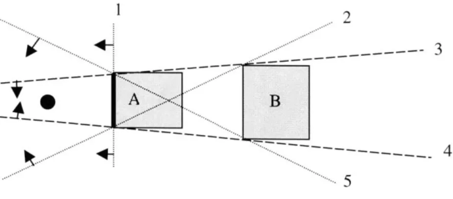
Given two objects A and B (see Figure 4), we discuss how we can detect if A occludes B. The first step is to compute the silhouette of both A and B as seen from the eye point. Secondly, using the silhouette points of A and B, we form supporting planes and separating planes as described in [10]. In Figure 4, lines 2 & 5 form the supporting planes while lines 3 & 4 are the supporting planes. Thirdly, we form a plane with the potential occluder, A, to ensure the eyepoint occluder is between the eyepoint and the occludee, B. In Figure 4, this plane is denoted by line 1. It is important to note that all planes are oriented towards the eyepoint. Finally, to test whether object A fully occludes object B, we test the eyepoint against the occluder plane and supporting planes (lines 1, 3 and 4 respectively). If the eyepoint is in the positive half-space of these three planes, we can conclude that A fully occludes B. It is important to note that the construction shown above only works with convex objects.

If A does not fully occlude B, we can test whether A partially occludes B.

Testing the eyepoint with each of the separating planes and the occluder plane

(20)

accomplishes this task. If all plane tests are positive, we can conclude that B is partially

visible with respect to A. This is important if there are other tests we can perform to see

which parts of B are visible and search to find objects that may occlude them.

If A does not fully or partially occlude B, we can conclude that B is visible with

respect to A as its occluder. However, we may find other objects in the environment to

occlude B. If no such object exists, we conclude that B is visible.

2.4 k-d Tree Hierarchical Data structure

As stated earlier, we are interested in accelerating the interactive rendering of

large computer graphics models. These large models could contain millions of polygons

spanned over several thousand objects. In the previous section, we described the

occlusion relationship between two objects. Since some models can contain many

objects, it would be inefficient to consider the visibility relationship between all pairs of

objects in the environment. Given n objects, we would have to perform at most n2

visibility computations. In order to deal with this complexity, we use a hierarchical data

structure known as a k-d tree [5].

A k-d tree is a binary tree data structure that has been historically used for storing

a finite set of points from a k-dimensional space. We are using the k-d tree to store our

objects (that are contained of points) in our 3-dimensional environment. Our k-d tree is

constructed as a hierarchical decomposition of the volume that defines the objects in our

environment. At each level of the decomposition, a split plane is chosen to divide the

(21)

objects according to criterion. We typically seek to divide the number of objects on each

side of the partition into equal parts. The decomposition occurs recursively until the

maximum level of recursion is reached, a minimum number of objects is obtained or

there are no other objects to split.

Each level of the decomposition constitutes a node in the binary tree. Each node

of the k-d tree is either a root, internal or leaf node. As with binary trees, every k-d tree

can only have a single root. The root node defines a boundary around all objects in the

scene. Internal nodes correspond to the various internal levels of decomposition. Finally,

the leaf nodes define the lowest of decomposition. Each leaf contains a list of objects

that intersect its boundary.

0 5 2

Figure 5 k-d Tree

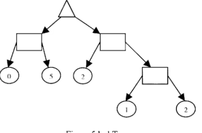
Figure 5 shows an example of a k-d Tree. The triangle node denotes the root of

the tree. Since the k-d tree is a binary tree, each node has zero or two child nodes.

Internal nodes in the tree are denoted by the squares. As internal nodes, they represent

various levels in the hierarchical decomposition of the 3D space. The circle nodes with

numbers inside of them denote leaf nodes. The number denotes the size of list of objects

(22)

that some objects may cross boundaries and are listed in more than one list. We can

reason that the k-d tree shown above has no more than 10 objects in the environment due

to potential overlaps.

As discussed in the previous section, we can determine if a single convex object

occludes another convex object. We can also determine in a similar fashion if a single

convex object occludes a node (or cell) of the k-d tree. Since a cell of the k-d tree is

denoted by a bounding box representation, it constitutes a convex object. If we determine

that a single convex object fully occludes a cell, we can conclude that all objects fully

contained in that cell are also occluded. Using the k-d tree helps to accelerate visibility in

the case where a single object occludes many objects close in proximity. By using k-d

cells, a single visibility computation can discern the visibility relationship between

(23)

Chapter 3: System Architecture

In this chapter, we will describe the key system components and algorithms of the

Distributed Visibility Servers system.

3.1 Model

In this section, we will describe the best types of models used for the Distributed

Visibility Server (DVS) System and any pre-processing needed before visibility

computation can occur. The DVS system works best with models with static objects.

Our visibility algorithms utilize spatial coherence with respect to the visibility it

computes and assumes occluders or subsequent occludees will not move in the

environment. It is possible to have dynamic objects in an environment used by our

system; however, our system will not compute visibility for these moving objects or use

them as occluders for other objects.

As stated earlier in this thesis, the DVS system is designed to accelerate visibility

computation for models containing a small number of occluder objects with respect to the

total number of objects in the environment. As we will describe in the next chapter, our

results are presented from a computer graphics model of the MIT campus. The MIT

model contains several large buildings that typically occlude a large percentage of the

(24)

contains over 1 million total polygons. In our experimentation, we used 40 occluders for

this model that contained over 600 objects.

Before visibility computation can begin, two preprocessing steps are performed:

k-d tree construction and occluder selection. The k-d tree precomputation step is

designed to create the k-d tree for the model a prior and store the tree in a binary output

file. This step is not a required step however it allows the client and the associated

servers to start faster. Since both the client and server need the k-d tree to compute

visibility, having the k-d tree precomputed accelerates that process. A precomputed k-d

tree also allows the client and server to communicate about the cells of the k-d tree with

the same tree structure. Otherwise, the client and server would have to synchronize on

the k-d tree construction algorithm (i.e. k-d tree max depth, splitting criterion, etc.).

The second precomputation step that is performed is Occluder Selection. This

step is designed to identify large potential occluder objects in the environment. While

this step could be performed automatically with a program with heuristics for selecting

potential occluders, we designed a non-automated program that allows users to create

occluders in the environment. Selecting occluders manually enables the user to select

simple convex occluders constructed from one or more complex objects containing

several thousand polygons. More information about the Occluder Selection module of

(25)

3.2 Region-to-Region Visibility

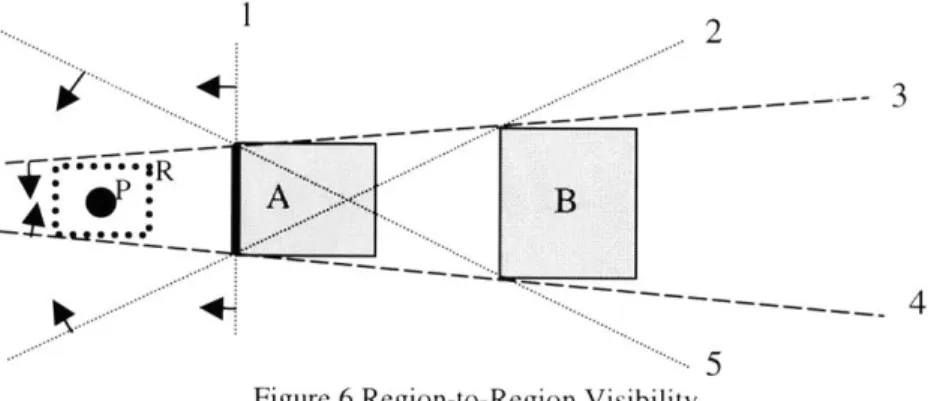
In Chapter 2 of the thesis, we discussed how a walkthrough client could determine if one object, A, occludes another object, B, from the user's point of view. In this section of the thesis, we will discuss how we can define a convex region that maintains the visibility relationship that object A occludes object B.

Region-to-Region visibility refers to computing visibility for an object that persists for a set of points in a region. As seen in Figure 6, the eyepoint, P, is enclosed in

a region, R. As long as the eyepoint remains inside this region, object A still occludes object B. This visibility relationship holds because all points of region R are in the positive half-space of the supporting planes 3 and 4.

.2

_A

B

Figure 6 Region-to-Region Visibility

The advantage of region-to-region visibility lies in its efficiency in determining if the visibility relationship defined by the region still holds. To determine if an object is still occluded, we must ensure that the point P is still in region R. This can be done efficiently with comparisons with the minimum and maximum points that define region

(26)

R. Without the region R, the eyepoint would have to be tested against all supporting

planes and occluder planes each time the user moves.

3.3 Algorithm

3.3.1 Overview

In order to accelerate the computation of visibility results for a walkthrough

client, both the precomputed k-d tree and pre-selected occluder files are needed. The

precomputation step is described in detail in section 3.1 Model.

In section 3.2 Region-to-Region Visibility, we described the basics of

region-to-region visibility. In order to find the region-to-region R for our visibility computation, we divide

the 3-D world into cubic regions of space (3D grid). For a particular region of space, we

resolve the visibility relationships of all k-d tree cells and that region. During real-time

walkthrough, as long as the eyepoint remains inside the region R, we treat the visibility as

constant. As soon as the eyepoint moves outside the region R, the visibility must be

recomputed.

5 While actual visibility relationships may change, we consider the visibility constant

(27)

Y

... _ ___ ._ vi.. ... _

.... ... ....

X

Figure 7 2D Visibility Cell Decomposition

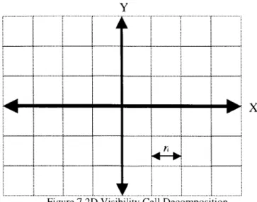
Figure 7 shows a grid layout of cells size nxn in 2-dimensional space. In

3-dimensional space, there would be cells extending n units high along the Z-axis.

Beginning at the origin, cells are defined according to cell size n. This single parameter

enables a consistent enumeration of all cells in the environment. Also, given the

eyepoint, it is straightforward to compute the min and max of the cell containing the

eyepoint. In Equation 1, we have listed the formulas for computing the minimum and

maximum points for the cell that contains the eyepoint.

CellMin.X Leye.X / nj * n CellMin.Y = Leye.Y/n I * n CellMin.Z Leye.Z in j* n CellMax.X = CellMin.X + n CellMax.Y = CellMax.Y +n CellMax.Z = CellMax.Z + n

(28)

3.3.2 Visibility Tree

In order to compute visibility for an entire region, we will use the k-d tree as a

tool to accelerate visibility. In this section of the thesis, we will outline the algorithms

used to compute visibility.

As mentioned in the preceding section, the Distributed Visibility Server (DVS)

system uses user regions to test visibility for objects and levels of the k-d tree spatial

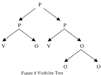
hierarchy. We use a visibility tree to record the visibility relationship between the user

region and the k-d tree. The visibility tree is a binary tree that is similar in structure-to

the k-d tree. At each level of the visibility tree, each node is one of three nodes: visible,

partially visible or occluded. We denote these three cell types as VCell, PCell, and

OCell respectively.

P

P P

V 0 V 0

0 0

Figure 8 Visibility Tree

In Figure 8 we show a sample visibility tree. We have abbreviated VCell, PCell

and OCell as P, V, and 0 respectively. This visibility tree would be returned as the result

(29)

3-dimensional environment, the rendering algorithm uses the visibility tree to determine the

visibility state of the k-d tree cells and objects in the environment. For example, view

frustum culling checks for intersection of k-d tree cells with the view frustum. If the cell

does not intersect with the frustum, objects inside that cell are culled from the rendering

pipeline. However, our occlusion culling algorithm checks the visibility tree for the cell

type. If the cell is classified as an OCell (occluded cell), the cell can be completely

culled from the rendering pipeline because all contained geometry is hidden. Otherwise,

it is successfully passed through the rendering pipeline.

3.3.2 Computing the Visibility Tree

In Appendix B, we list the recursive function for building a visibility tree. In

order to build the tree, the root cell of the visibility tree, the user region, a list of

occluders and eyepoint must be specified to the ComputeVisibilityTree function. The

Occluded function is a helper function designed to determine whether a generic BBox

region of space is visible from a user region given a list of occluders.

3.3.2 Computing Visibility Distributely

The graphics client uses the Distributed Visibility Server (DVS) system to

accelerate the computation of occlusion culling. When roaming in the environment, the

graphics client seeks to use view point predication to determine the next user region the

(30)

visibility from the visibility servers before the client enters the reason. If the user enters a

region that has no prefetched data, the client must compute the results locally.

The view point predication mechanism of the graphics client consists of a simple

directional test. While the eyepoint is in its current region, the predication algorithm

determines which neighboring cell the user would enter if he would continue moving

forward along a straight line. The next cell is determined by shooting a ray from the

eyepoint to the 26 neighboring cells of the current cell. The first cell the ray intersects is

the next cell. The client sends requests to the servers for the next predicted cell it

encounters. If the client has visibility information for a neighboring cell already cached,

a new visibility request is not sent. Additionally, if a visibility request is outstanding and

the results have not been returned, a new visibility request is not sent.

As the new visibility results arrive to the client, they are cached using a least

recently used (LRU) replacement strategy. The client has a maximum number of

visibility regions it can cache before visibility regions must be removed. Once the

visibility region is removed from the cache of the client, it must be requested again if the

(31)

Chapter 4: Results

In this chapter we highlight the performance of the Distributed Visibility Server

(DVS) system on our MIT campus model. In the experiment outlined below, we used

three (3) Dell 300 Mhz Windows NT workstations with 128Mb of RAM and 10Gb of

hard disk space. One of the Windows PCs served as the client workstation while the

other machines served as the server.

In order to study the performance gains of the DVS system, we ran our system

using four different setups using an identical camera path through the model. The first

setup was performed with no occlusion culling. This measurement is useful to

understand the baseline performance of the system. The second setup measured the

effects of performing view frustum culling only. View Frustum culling has been shown

to yield good results when the majority of the model is not in the field of view. We

studied this phenomenon separately. The third setup measured the effects of performing

view frustum culling locally and occlusion culling locally. This setup did not use any

visibility servers to accelerate occlusion culling. The final setup measured the effects of

performing view frustum culling locally and occlusion culling remotely. In this scenario, we used 2 visibility servers.

We will show three graphs. The first graph shows the draw time measured in

(32)

computing occlusion measured in milliseconds. Finally, the last graph shows the frame

rate of the four setups.

4.1 Draw Time

M, E Draw ime 20D00 1800 1600- 1100-12DO 1000 600 aMot 0

0 rOC - 10 LO~ M N~C~ 0 MO WO N WO 'IT M N~ ;'-0 0M M r- WO LO It M~ N\ 0 03) 00

N-CM LO O 1q Nl- 0 CO CO 0) j It r N 0 CO WO 0) Cdj tOO CO) (O 0) 01 LO 00 - t 01 N- LO M

CJCCJC C'ITOC 'IT LO LO

Frame -Nome -25 per. Mo. Ag (VF) -- 25 per. Mov. Ag (VF/Occ

Figure 9 Drawing time

(local)) -25 per. Mov. Ag. (VF/Occ (2 retae))

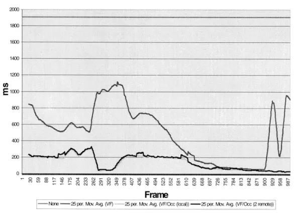
Figure 9 shows the draw time of the four setups of our experiment. The time is measured in milliseconds for each frame along camera path. In this graph, it is important

(33)

Server (DVS) significantly reduced the draw time for both locally and remotely computed occlusion culling. The plot of the draw time for the local and remotely computed visibility is nearly identical. Since the amount of geometry drawn should not vary based on where visibility was computed, this is what we would expect for the draw time.

4.2 Occlusion Culling Time

Occlusion Cull Time

200 180 160 140 120 U) E 100 80 60 40 20 0

M r- 01 _C'4to _couO t -Mo _LO~ (0 M~ -) LO C1 o Mo 0 M r CM - (0 no 0M MO N M It 1- N- 0 t C) CO (0 - 0) 0 t-- - to) 't C) N- C'J o0) U to -~ to) to - m 0 0) CD 0 O L C0O

01\ 1 1 CO CO) COce CO) lzr L0 to Lr O to to ) CD r0 rO-N-N- o o aoo ) a)0a)

Frame

25 per. Mov. Avg. (VF+Occ (local)) 25 per. Mov. Avg. (VF+Occ (2 remote))

Figure 10 Occlusion culling time

(34)

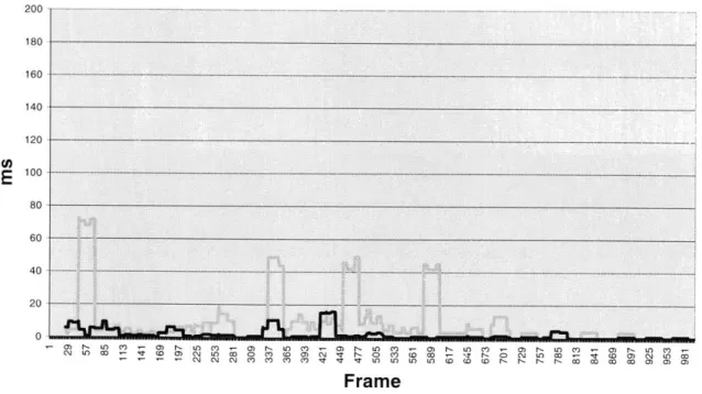
-Figure 10 shows the time spent on two of the four setups that used occlusion

culling in our experiment. The time is measured in milliseconds for each frame along

camera path. It is important to note that the time the local occlusion culling graphics

client spent computing visibility was significantly higher than the time for the client

using remote visibility servers. There are a few spikes in the plot for the client using

remote resources. These spikes are due to visibility results not being available for the

graphics client. This phenomenon could be due to slow view point predication or slow

network connectivity. The time noted during these spike represents the time the client

(35)

4.3 Frame Rate Comparison

Frame Rate Comparison

U-Mi 30 25 20 15 10 0) C2 0): N- ro N- U) 0 ) N ) 0 M) ) N L- U M) ) M) 0 - LO U )- LO M) - ~ N- N- N- j M))0 M 0 M 4 I 't U) )MUO (0 to0 r,- N- N- N- M0(M (M(M0M0M0M Frame

I None - 25 per. Mov. Avg. (VF Only) -=-25 per. Mov. Avg. (VF+Occ (local)) - 25 per. Mov. Avg. (VF+Occ (2 remote))

Figure 11 Overall Frame rate

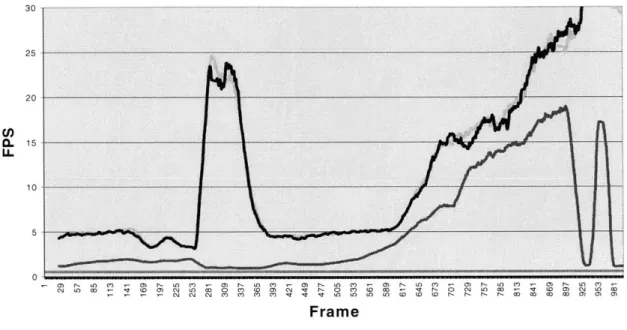
Figure 11 shows the frame rate measurement for the graphics client for our 4 setups. It is important to note that both setups that contained occlusion culling outperformed the setup with no culling and the setup with view frustum culling only. Of the two setups that contained occlusion culling, the frame rate plots are nearly identical. Upon closer inspection, the plot of the client utilizing remotely computed visibility did out perform the client using locally computed results in several key places. While this particular plot does not suggest that computing visibility remotely offers significant gains, we believe our system will achieve significant performance improvements using a model that has more demanding occlusion culling properties. Additionally, the future

(36)

work section of the thesis provides insight into other possible configurations that can also

(37)

Chapter

5:

Conclusions

This thesis showed that employing remote visibility servers to compute

conservative visibility is an effective technique in increasing the rendering performance

of a single walkthrough client. The Distributed Visibility Server (DVS) system was

designed to accelerate the visibility computation of graphics clients in a walkthrough

environment. We have described the design and implementation of the visibility servers.

Also, we have studied the performance of the servers using a model of the MIT campus.

We have presented results confirming the occlusion culling algorithms

implemented in this thesis have significantly increased the rendering performance of

non-visibility computing graphics clients in a walkthrough environment. Additionally, we

compared the occlusion culling times of two visibility computing walkthrough clients.

One client computed visibility locally while the other used the visibility servers when

possible. Our studies showed that the client using the visibility servers spent 79.5% less

time computing occlusion culling than the client computing visibility locally. However, when comparing the rendering performance of a graphics client computing visibility

locally versus remotely we did not observe significant performance increases when using

two servers. Due to communications bottleneck, the rendering throughput of our system

did not improve significantly. Our detailed statistics suggest that the client using the

(38)

updates from the remote visibility servers. In order to increase the rendering

performance, the amount of time spent communicating with the server must be less than

the amount of time spent computing visibility.

In this thesis, we have outlined one possible configuration of the visibility server

system with graphics clients. In our experiment, we used one client with two visibility

servers. However, there are other visibility server configurations that can substantially

increase the rendering performance of walkthrough clients. These configurations are

(39)

Chapter 6: Future Work

In the previous chapters, we have discussed the feasibility of the Distributed

Visibility Server system to accelerate the computation of visibility for a walkthrough

graphics client. The system we developed works with static environments that have a

small number of large occluders. Throughout this thesis, we have discussed a

configuration of our system that consists of one or more visibility servers and a single

graphics client. In this chapter, we will discuss two other possible configurations. These

configurations allow visibility information to be cached between rendering clients and

may offer additional computational benefits.

6.1 Multiple Clients

The first configuration consists of multiple walkthrough clients operating in the

same static environment with visibility servers. Currently, each client is responsible for

opening a connection to the server and sending visibility requests. Since both the client

and server were developed using the client-server architecture much like traditional

WWW servers, it is possible for one or more servers to serve multiple clients. This

works particularly well in the case of two clients operating in the same environment

because visibility results can be cached from client to client similar to web pages for a

(40)

For example, assume two clients, client A and client B, are operating in the same

environment. If the clients are in close proximity to each other, it is possible for client B, to enter a visibility region that was previous occupied by another client A. If this

happens, client A would first request and receive the visibility results from the server.

However, when client B requests the same visibility information for the same region, the

server will not have to recompute the results. The server can simply store the results in a

look-up table and send the results to client B without recomputation.

6.2 Multiple Clients, No Servers

The second configuration consists of multiple walkthrough clients in the same

static environments with no visibility servers. In this scenario, no dedicated servers

would be used to compute visibility information. However, since the clients are

operating in the same visibility environment, it is possible for the clients to share

visibility computation. This configuration is possible if the clients send visibility

requests to each other instead of dedicated servers. It would be interesting to measure the

(41)

Appendix A: Implementation

In order to study the performance of using a set of distributed visibility servers in

this thesis, a number of hardware and software technologies were used. In this section of

the thesis, we will discuss the hardware and software technologies used.

Al. Software Technologies

All software for the visibility servers and the graphics client were written using

Sun Microsystems's Java 2 Programming Language [1] (see http://java.sun.com for more

information). Our rendering client used the optional Java3D rendering API. Java3D is a

package available for Java programs to render 2D and 3D scenes. Java3D has

capabilities for building a scene graph and a mode for immediate mode rendering.

Java3D has both OpenGL and Microsoft Direct Draw bindings. Our system used the

OpenGL bindings with an Intergraph Intense 3D Pro board discussed in the Hardware

Technologies selection below.

The test model used in this thesis was in the Virtual Reality Markup Language

(VRML) [7]. A VRML loader is contained in the Java3D package. Therefore, no custom

(42)

A2. Hardware Technologies

Since all of the software was written using the Java programming language and

supporting packages, we could have run our system on a host of hardware platforms.

However, in order to eliminate any performance variations from using heterogeneous

components, we decided to run our experiment on similarly configured workstations.

Most of our visibility servers were Dell Computer Corporation 300 Mhz

Windows NT workstations with 128Mb of RAM and 10Gb of hard disk space. Since our servers stored cached visibility results, RAM proved to be a factor that could affect the performance of our visibility computation. Through experimentation with the graphical models we were using, we found that 128MB for our servers was reasonable.

Our rendering client was also a Dell Windows NT workstation with 128MB of RAM, 10Gb of hard disk. We added an optional Intergraph Intense 3D Pro OpenGL hardware accelerated board. This board allowed us to render over 3 million polygons per second. The optional graphics board enabled us to use a graphics model that contains several million polygons.

A3. Running the system

In order to take advantage of the remote compute resources of the visibility servers, both the client and the servers must be started on their respective machines. In this section we will describe how to start the k-d tree precomputation, occluder selection, client and server programs.

(43)

A3. 1. Running the KD Tree Precomputation Program

The k-d tree precomputation program is responsible for computing the k-d tree for

both the client and the server to use. Precomputing the k-d tree enables the client and the

server to start faster and ensure both programs are assuming the same k-d tree. This is

important when a server is computing visibility for a client that should have the same k-d

tree structure.

C:\>

java

precomputeKDTree #levels inputFile OutputFile

In order to start the k-d tree precomputation, three parameters are needed. The

first parameter denotes the maximum number of levels to recurse when creating the k-d

tree. The second parameter denotes the input file model file. The third parameter denotes the output file for the binary k-d tree.

A3.2. Running the Occluder Selection Program

The Occluder Selection program is designed to allow the user to manually select

occluders in the environment. The Occluder Selection program needs one input

parameter, the input file. The program loads the input model and allows the user to interactively create occluders for the model.

(44)

C:\> java occluderselection inputFile

Figure 12 Occluder Selection Option

Figure 12 shows the options dialog box for the Occluder Selection program. The

options box contains several parameters for specifying occluders in the environment. For

example, the Geometry Objects widget, allows the user to select the set of objects to draw

in the output window. Using this parameter, the user can select a set of potential occluder

objects and later use the 'Add Box' button to create a new occluder. The sliders at the

bottom of the options window allow the user to resize the newly created box. Figure 13

(45)

allows the user to spin and rotate the model in view. Below we show the model we used

for the interactive walkthrough application.

Figure 13 Occluder Selection Trackball View

A3.3. Starting the Server

The Visibility Server is responsible for providing visibility results for one or more

graphics clients. In order to provide the results, the visibility server must be given some

configuration information about the environment the client will be operating in. Below is

a table listing the different options a visibility server receives. These options are fed to

the server in a text-based configuration file.

(46)

Options

Description

KDTREEURL Specifies the URL location of the pre-computed KD-Tree.

NUMKDLEVELS Specifies the number of levels for the pre-computed KD-Tree.

OCCLUDERURL _{Specifies the URL location of the pre-computed occluders for this database.} NUMTHREADS _{Specifies the numeric value for the number of threads for this server.} PORT _{Specifies the port the server will list for visibility request on.}

Table 1 Description of Server Options

The following instruction assumes the server will be started on a Windows-based

PC 6. _{Given a text-based option file with the values specified in Table 1, the visibility} server is started from the command as follows:

C:\>

java

visibilityServer confirmation. file

After the above command is executed, the visibility server will first load the pre-computed KD-Tree and Occluder Database file. Secondly, it will create the number of threads specified by NUMTHREADS value. Finally, it will wait for incoming request

by the client to compute visibility information.

A3.4. Starting the Client

The Client is responsible for rendering the scenes according to the navigational input specified by the user. In order to provide rendered scenes, the client must be given configuration information about the environment the client will be operating in. Below is

(47)

a table listing the different options a client receives. These options are fed to the client in

a text-based configuration file.

Options

Description

ENABLESTATS This Boolean option toggles general statistics are turned on/off.

ENABLEFRSTATS This Boolean option toggles frame rate statistics on/off.

ENABLEMEMSTATS This Boolean option toggles memory statistics on/off.

ENABLECTSTATS This Boolean option toggles computer time statistics on/off.

ENABLEOCCSTATS This Boolean option toggles occlusion statistics on/off.

WALKFARPLANE Specifies the walkthrough camera far plane.

TRACKFARPLANE Specifies the trackball camera far plane.

MAXWALKSPEED Specifies the walkthrough camera maximum velocity.

WALKSPEED Specifies the walkthrough camera speed.

TRACKSPEED Specifies the trackball camera speed.

MAXTRACKSPEED Specifies the trackball camera maximum speed.

FILE Specifies the file (on the internet) to load. This option is a URL value.

KDPRECOMPUTE Specifies a file for a pre-computed KD-Tree.

KDVIZPRE Specifies a file for pre-computed KD-Tree visibility information.

SHOWKDVIZ This Boolean option toggles KD-Tree visualization on/off.

KDLEVELS Specifies the number of levels to build the KD-Tree.

KDSLEEP Specifies the number of milliseconds to sleep during KD-Tree construction.

DRAWTRACK This Boolean option toggles draw trackball mode on/off.

DRAWWALK This Boolean option toggles draw walkthrough mode on/off.

DRAWVIZ This Boolean option toggles draw visualization mode on/off.

SERVERS Specifies a list of visibility servers to client uses.

CONTACTSERVER This Boolean option toggles contact server on/off.

DEBUGMODE This Boolean option toggles debug mode on/off.

GRIDSIZE Specifies the grid size for the client to request visibility information.

NUMRECTHREADS Specifies the number of threads the client program use to receive information from the server.

CAMERAPOS Specifies the camera initial position (X, Y, Z).

CAMERAHEADING Specifies the camera initial heading (in radians).

CAMERAPITCH Specifies the camera initial pitch (in radians).

CAMERALOG Specifies the file to save the camera position data in.

PERFLOG Specifies the file to save the performance data in. Table 2 Description of Client Options

6 The following MS-DOS instruction assumes the proper Java Classpath and supporting libraries have been properly specified.

(48)

Given a text-based option file with the values specified in Table 2, the client is

started from the command as follows. The following instruction assumes the client will

be started on a Windows-based PC7.

C:\>

java

Visibilityclient confirmation.file

After the above command is executed, the client will first load the pre-computed

KD-Tree (if available) and the geometry database. Secondly, it will create the number of

server threads specified by NUMRECTHREADS value. Finally, render the scenes

based on the navigation input from the user and send out visibility request to the specified

visibility servers.

Figure 14 Client Rendering Performance Window

7 _{The following MS-DOS instruction assumes the proper Java CLASSPATH and}

(49)

In order to study the performance of the client application, we

incorporated real-time statistics gathering tools for measuring rendering performance. In

Figure 14, we have a screen shot of the client application rendering statistics. The

rendering statistics are split into four sections: database rendered, timing, memory and

server occlusion task history. The database rendered section allows the user to observe

the percentage of the database that is view frustum culled, occlusion culled and sent to

the rendering pipeline. The timing section allows the user to observe the percent of time

spent culling the database and rendering geometry. The memory section allows the user

to monitor the memory used during the application. The server occlusion task history

allows the user to monitor the number of occlusion tasks sent out and received. These

statistics are useful in debugging the application and allowing introspection into the code.

(50)

Figure 15 shows a bird's eye view of the walkthrough client application. This view allows the user to visualize the internal characteristics of the visibility algorithm. In the view above, the view frustum of the user is shown in yellow (transparent). Several white and yellow wire frame boxes are overlaid on the model. The wire frame boxes represent cells of the k-d tree subdivision. The green k-d cells intersect the view frustum and are potentially visible. The white boxes represent k-d cells that do not intersect the view frustum. Figure 16 shows the configuration of the program for the view in Figure

15. In this particular run of the program, view frustum culling was turned on for both

cells of the k-d tree and objects. However, occlusion culling was turned off. If occlusion culling was turned on and cells were invisible, Figure 15 would show occluded cells drawn in red.

(51)

Figure 16 Client Rendering Options Window

(52)

Appendix B: Visibility Tree

ComputevisibiIityTree(KDTree cell, BBox regionBBox, List Occluders, Point eye)

{ if (cell.type == PARENT) if (occluded(cell.BBoxO, regionBBox, Occluders, eye) return OCell; }

KDTree left = cell.getchild(left);

KDTree right = cell .getchild(right);

leftResult = computevisibilityTree(left, regionBBox, Occluders, eye)) rightResult = computevisibilityTree(right, regionBBOX, Occluders, eye))

if (leftResult == OCell && rightResult == OCell)

{

return OCell;

}

if (leftResult == VCell && rightResult == VCell)

{ VCell.left = leftResult; vCell.right = rightResult; return VCell; } PCell.left = leftResult; PCell.right = rightResult; return PCell; } else { // CHILD cell

for each object o in cell

{ if (occluded(o.bbox), regionBBox, Occluders, eye)) Mark o as occluded } }

(53)

return VCell;

} }

Occluded(BBox occludeeBBox, BBox regionBBox,

List Occluders, Point eye)

{

// Define a ray from region to occludee center Point occCenter = occludeeBBox.center(;

Point regioncenter = regionBBox.center(; Vector ray = occCenter - regionCenter;

// Potential occluders

List potentialoccluders = gather(occluders,

ray,

regioncenter); for each potentialoccluder P {

Plane[] vizPlanes = computevizPlanes(eye,

occludeeBBox, P); if (eye.inPositiveHalfspace(vizPlanes) return TRUE; } return FALSE; } 53

(54)

Bibliography

[1] _{Arnold, K., Gosling, J. and Holmes, D. The Java Programming Language,}

Third Edition. Addison Wesley, 2000.

[2] Airey, J. M., Rohlf, J.H., and Brooks, Jr., F. P. Towards Image Realism with Interactive Update Rates in Complex Virtual Building Environments. ACM

Siggraph Special Issue on 1990 Symposium on Interactive 3D Graphics 24, 2

(1990), 41-50.

[3] Akeley, K. RealityEngine Graphics. SIGGRAPH '93 Conference Proceedings (1993), 109-116.

[4] Arpaci, R., Vahdat, A., Anderson, T., and Patterson, D. Combining Parallel and Sequential Workloads on a Network of Workstations. Technical report, Computer Science Division, University of California at Berkeley, 1994.

[5] Bentley, J. L. Multidimensional Divide and Conquer. Communications of the

ACM, 23 (4): 214-229, 1980.

[6] Basch, J., Guibas, L., Silverstein, C., and Zhang, L. A Practical Evaluation of

Kinetic Data Structures. Proceedings of the 13th International Annual Symposium of Computational Geometry (SCG-97), 1997.

[7] Beeson, C. An Object-Oriented Approach To VRML Development. VRML

97: Second Symposium on the Virtual Reality Modeling Language, ACM

Press, February 1997,

[8] _{Catmull, E. E. A Subdivision Algorithm for Computer Display of Curved}

Surfaces. PhD thesis, University of Utah, Dec. 1974.

[9] Coorg, S., and Teller, S. Temporally coherent conservative visibility. In

Proceedings of the 12th Annual ACM Symposium on Computational Geometry (1996).

[10] Coorg, S., and Teller, S. Real-Time Occlusion Culling for Models with Large

Occluders. In Proceedings of the Symposium on Interactive 3D Graphics (1997).

(55)

[11] Greene, N., Kass, M., and Miller, G. Hierarchical Z-buffer visibility.

SIGGRAPH '93 Conference Proceedings (Aug. 1993), pp. 231-238.

[12] Greene, N. Hierarchical polygon tiling with coverage masks. In SIGGRAPH

96 Conference Proceedings (Aug. 1996), ACM SIGGRAPH, Addison

Wesley, pp. 65-74.

[13] Funkhouser, T., Sequin, C., and Teller, S. Management of Large Amounts of Data in Interactive Building Walkthroughs. In Proc. 1992 Workshop on

Interactive 3D Graphics (1992), pp. 11-20.

[14] Hudson, T., Manocha, D., Chohen, J., Lin, M., Hoff, K., and Zhang, H. Accelerated occlusion culling using shadow frusta. In Proc. 13th Annual

ACM Symposium on Computational Geometry (1997), pp. 1-10.

[15] Luebke, D., and Georges, C. Portals and mirrors: Simple, fast evaluation of potentially visible sets. In 1995 Symposium on Interactive 3D Graphics (Apr. 1995), P. Hanraham and J. Winget, Eds,. ACM SIGGRAPH, pp. 105-106. ISBN 0-89791-736-7.

[16] Naylor, B.F. Partitioning Tree Image Representation and Generation from 3D geometric models. In Proc. Graphics Interface '92 (1992), pp. 201-221.

[17] Sutherland, I. E., Sproull, R. F. and Schumaker, R. A. A. Characterization of Ten Hidden-Surface Algorithms. Computing Surveys 6, 1 (1974), 1-55.

[18] Teller, S., and Alex, J. Frustum Casting for Progressive, Interactive Rendering. MIT LCS TR-740.

[19] Teller, S., and Sequin, C. H. Visibility preprocessing for interactive walkthroughs. Computer Graphics (Proc. Siggraph '91) 25, 4 (1991), 61-69. [20] Zhang, H., Manocha, D., Hudson, T., and Hoff III, K.E. Visibility culling

using hierarchical occlusion maps. In SIGGRAPH 97 Conference

Proceedings (Aug. 1997), T. Whitted, Ed., Annual Conference Series, ACM

Distributed visibility servers

Distributed Visibility Servers

Distributed Visibility Servers

Abstract

Acknowledgements

Contents

List of Figures

List of Tables

List of Equations

Chapter 1: Introduction

1.1 Overview

1.2 Motivation

1.3 Related Work

1.4 Organization of Thesis

Chapter 2 Background

2.1 Visibility Computation

2.2

Traditional Rendering Pipeline

2.3 Occlusion Culling in 2D

A1Y

B

77i

4

2.4 k-d Tree Hierarchical Data structure

Chapter 3: System Architecture

3.1 Model

3.2 Region-to-Region Visibility

B

3.3 Algorithm

3.3.1 Overview

X

3.3.2

Computing the Visibility Tree

3.3.2 Computing Visibility Distributely

Chapter 4: Results

4.1 Draw Time

4.2 Occlusion Culling Time

4.3 Frame Rate Comparison

Chapter

5:

Conclusions

Chapter 6: Future Work

6.1 Multiple Clients

6.2 Multiple Clients, No Servers

Appendix A: Implementation

Al. Software Technologies

A2. Hardware Technologies

A3. Running the system

A3. 1. Running the KD Tree Precomputation Program

java

Options

Description

C:\>

java

Options

Description

C:\>

java

Appendix B: Visibility Tree

Bibliography