Digital data processing techniques for radar mapping.

ESL-TM-343

DIGITAL DATA PROCESSING TECHNIQUES FOR RADAR MAPPING

by

Robert W. Roig January, 1968

Contract No. AF-33(615)-3227

This technical memorandum consists of the unaltered thesis of Robert W. Roig, submitted in partial fulfillment of the requirements for the degree of Doctor of Science at the Massachusetts Institute of Technology in January, 1968. The research reported herein was conducted by the author at the M. I. T. Electronic Systems Laboratory under a National Science Foundation fellowship grant. The publication of this work was

made possible through the support extended to the Massachusetts Insti-tute of Technology, Electronic Systems Laboratory, by the United

States Air Force (Avionics Laboratory, Research and Technology Divi-sion), under Contract No. AF-33(615)-3227, AF Task No. 504211, M. I. T. Project DSR 76143. This report is published for technical in-formation only, and does not represent recommendations or conclusions

of the sponsoring agency.

This document is subject to special export controls, and each transmittal to foreign governments or foreign nationals may be made only with prior

ap-proval of the Air Force Avionics Laboratory (AVNT), Wright-Patterson Air Force Base, Ohio.

Electronic Systems Laboratory Department of Electrical Engineering

Massachusetts Institute of Technology Cambridge, Massachusetts 02139

DIGITAL DATA PROCESSING TECHNIQUES FOR RADAR MAPPING

by

ROBERT W. ROIG

S.B., Massachusetts Institute of Technology (1950)

S.M., Massachusetts Institute of Technology

(1958)

E. E., Massachusetts Institute of Technology

(1964)

SUBMITTED IN PARTIAL FULFIILMENT OF THE REQUIREMENTS FOR THE DEGREE OF

DOCTOR OF SCIENCE

at the

MASSACHUSETTS INSTITUTE OF TECHNOLOGY January 19 68

Signature of Author ___ -' /t_ *.

Department of Electrical Eg.ineering, January 17, 1968

Certified by

7.

Thesis Co-Supervisor

Thesis Co-Supervisor Accepted by

by

ROBERT W. ROIG

Submitted to the Department of Electrical Engineering on 17 January 1968 in partial fulfillment of the requirements for the Degree of Doctor of- Science.

ABSTRACT

Alternatives for the organization of the data processing problem for high quality radar mapping are examined under the constraint of a "digital" implementation. The comparison is made on the basis of the functional requirements that each formulation, of the organiza-tion problem, places on the implementing apparatus. Quantizaorganiza-tion effects on the quality of the radar maps produced, are studied by generalizing the "spread function" quality indication of linear radar theory to a statistical measure, termed the "M" function. This is essentially the covariance between the radar map function and the scatterer density function which gives rise to the radar signals. It is shown that the "Ml" function is computable in useful form for

a radar in which the data is quantized. The results show that a quantizer step size equal to the rms quantizer input will be adequate in most cases of practical interest.

The sis Co -Supervisor s Godfrey T. Coate

Lecturer in Electrical Engineering Alfred K. Susskind

Associate Professor of Electrical Engineering

A CKNOWLEDGEMENT

I wish to thank the National Science Foundation, whose support in the form of a fellowship grant, made this research effort possible. The stimulation and encouragement of Mr. Godfrey Coate in the radar aspects and Professor Alfred Susskind in the digital aspects were vital to the successfful completion of this research effort. To them, and Professor J. Francis Reintjes, who served as a reader on my thesis committee, I express my sincere thanks. Especial thanks are due to Miss Sandra Botelho who did a remarkable job of

typing the finished manuscript directly from my not-too-legible script. The encouragement and support of the entire

staff of the M. I. T. Electronic Systems Laboratory, were invaluable. Professor George C. Newton, who has guided my academic career at M. I. T. owns my especial gratitude.

Abstract Page ii Acknowledgement iii List of Illustrations v List of Symbols vi I. INTRODUCTION A. Objectives 1

B. Background and Motivation 2

C. Summary of Results 8

II. A MODEL OF THE RADAR MAPPING PROBLEM 15 III. ALTERNATIVES FOR ORGANIZATION OF : 40

DATA PROCESSING

IV. QUANTIZATION EFFECTS 52

V. COMPARISON OF THE IMMEDIATE AND 94

DELAYED FORMULATIONS FOR DIGITAL IMPLEMENTATION

APPENDIX A 108

A Spatial Model of Radar Signals for Realistic Geometries

APPENDIX B 117

Joint Characteristic Functions of Quantized and Continuous Random Variables

APPENDIX C 121

Computation of the "M" Functions for Radars with Quantized Data Channels

BIB LIOGRA PHY 138

BIOGRAPHICAL NOTE 13 9

LIST OF ILLUSTRA T IONS

1 Radar Mapping Geometry Page 31

2 . 'ua (t) Mapping 33

3 Delayed Processing 42

4 Immediate Processing 44

5 Quantizer 53

6 Variations in Data Quantization 55

7 Sketch of Effective Tapering vs. Actual 77 Tapering

8 Processing Apertures 82

9ad.L) pulse amplitude modulation' function

A aperture area

Ad_dm am -d) _d overlap area of

point-scatterer-signal-function and proce ssor-weighting-function apertures in

signal space.

AL area under main lobe of L

(

;u )'

also area of resolution cefiin n certain cases.

''A normalizing.constant in statistical

model of U m)

As sampling area in signal space

c radiation propagation velocity

C(uLd; u) part of Md; um) due to quantization

CR range compression ratio

CS azimuth compression ratio

e(t) transmitted signal (in complex

analytic form)

e u) (t; 'received signal due to unit point scatter located at u

m

The general scheme of notation is as follows: overscores indicate a set of coordinates; an underscore indicates a complex quantity ~ lack of

an underscore indicate a real quantity; the real and imaginary parts of a complex quantity are indicated by subscripts 1 and 2 respectively attached to the same symbol as the complex quantity but without under-scores, i.e. e (t) = e (t) + j e 2(t). The subscript q indicates a

quantity that has been sampled and quantized; the subscript s indicates a quantity that has been samplead but not quantized.

E (t) received signal

E;

LL6iJU)

f (t; d ) temporal weighting function for

map point ud

g9(t) antenna gain at tithe: t relative

toe unity.for scatterer at u

m

G (S) geometrical attenuation factor

'relative to unity:for 'scatterer at :u and radar at S.

h(t, t'; u) response at time t from a unit

point scatterer located at u , to an impulse transmitted at time t' iCUa XUH;

um)

response at ua from a unit point

scatterer located at u , to an m

impulse transmitted from u '

I (ud)

complex map function

c.>n 65

1:

.imaginary part of

K a'u; ud) spatialweighting function for mapspatial weighting function for map point ud

L m(U; u3) Inverse matched smoothing function

M(Ud; Um)'" correlation coefficient of Y(Um) 2 andtI(ud)12 defined as the radar map quality function.

n(t) noise component of E (t)

-- N(ud)

component of I(u

d )

due to noise

vii

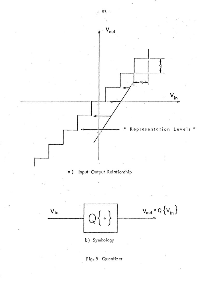
Q4,*9·3~~~

~quantization

operator

q quantizer step size

Real part of

tRmx(t) Mdistance- from antenna to u

at time t

R

(S)

distance from antenna to u

x when radar is at S m

R propagation distance coordinate

of signal space

Ra = T =propagation distance

a 2p

aperture

Rd "range" coordinate -of map space

RM Rx,R "range" coordinate of scatterer space

S . trajectory distance coordinate of

signal space

S trajectory distance aperture

a

S "azimuth" coordinate of map space

S "azimuth" coordinate of scatterer

m

space

S radar position along trajectory at

time of transmission of nth pulse

t time

T(u -u ) scatterer density correlation

X y-'

fuinc

tion

T reference time or time of

trans-n mission of nth pulse

T transmitted pulse length

p

u,, ux, UY scatterer space coordinates

u U_S signal space coordinates

d . map space coordinate

un ( t ) mapping of t onto a

one-dimensional subset bf signal space.

U speed along the trajectory

0 I

v r(U%;u) spatial model of received

signal from unit point scatterer

at u

in

Vr(Ua: )spatial model of received signal

V 2r/q = quantizing "frequency"?Z;

(VR) ratio of the volume under the

incoherent part of

Mi(d;

um ) to the volume under' the side-.

lobes of the dominant part

w('; ud) weighting function amplitude

or "aperture" function

w:w

₂

,

3

,w

4

amplitude wei'ghtings due to

quantization

Wa(Ua; d) effective amplitude weighting, for

dominant part of M(u'd;-u), due to quantization "after-the -multiplier ".

W spatial bandwidth in radian measure

P

ratio of bit storage capacity required

for immediate formulation of process-ing to that required for the delayed fo rmulation

mrnatched" processor

r-

Ud smoothing function for a

quantized weighting function

(but without data quantization)

b(8u -u )

Dirac delta function in one or

x m

more dimensions

l]~(u.) - - spatial noise component of

-r (U0)

AX wavelength

dummy time variable

(uva; ud) product of V (u ) and K*(UC; ud)

pulse phase modulation function

(ua) -. equivalent phas-e- error due to

quantiz ation

complex scattering coefficient for a point scatterer located at

rn

y(um) scatterer density function

I. INTRODUCTION A. Objective

The purpose of the research reported in this thesis has

been to develop analysis techniques which would be useful in the

design and evaluation of fine-resolution radar mapping systems in which the extraction of map data from signal data is accomplished "digitally". By this we mnlean systems in which the data manipulation or "processing" is accomplished, at least in part, on digitized

number representations of the data. Specifically, we have sought and attained useful results in

(l)Modeling radar signals, particularly the conversion frorm "temporal" to "spatial" models of the signals encountered in air-borne mapping radars.

(2)Organizing the data-processing operations and identifying tweo competing formulations of data processing for detailed study.

(3)Determining the effects of quantization of radar data on radar mapping performance by generalizing the conventional "spread function"

(or spatial impulse response) criterion of radar performance to a statistical performance function which is calculable for "quantized" data processing.

(4)Specifying the functional requirements which various radar performance objectives will impose on the implementing digital apparatus .

"pulse-coLnpres sion, synthetic-aperture" type, intended for use in .making "fine-resolution" maps of the earth's surface from a moving

vehicle, in particular an aircraft. As is well known, the "synthetic-aperture" radar obtains an improvement in azimuth resolution over a conventional radar by performing a weighted, coherent summation of the received signals over an interval of time during which the carrier vehicle moves an appreciable distance. This summation is comparable to that accomplished by a real antenna on the field vectors in its

physical aperture; hence the term "synthetic aperture". The first-order theory of such radars is well understood and operating models have been constructed. 2 5

Existing. implementations of combined synthetic aperture and pulse compression radars are almost exclusively in the domain of analog apparatus, with the optical processor the most successful to date. In operation, the radar data processor must accomplish a

separate summation for each resolvable element in the map finally obtained. The rate at which resolvable elements can be scanned by

synthetic-aperture radars, carried on modern aircraft, is very high, being upwards of 10 resolvable elements per: second. The time duration

of the radar signals which enter into the summation pertinent to a single resolvable element is relatively long by electronic standards, being on

the order of seconds. These facts have combined to make high-density analog signal storage media, such as photographic film, a prerequisite for successful implementation of analog processors.

The first-order theory of synthetic aperture radars shows that the required summation is very similar to the computation of a Fourier transform, an operation which optical systems can perform quite naturally and accurately on signals recorded as photographic

.trans-parencies. Hence, the present pre-eminence of optical processors. There are two areas of application of fine-resolution mapping radars where optical processors have some serious disadvantages. One is in the area of "real-time viewing" of processed radar data, i.e. on the aircraft carrying the radar. In fact, optical processing of radar data is customarily done at a ground-based facility, due to the difficulties involved in the mechanical and chemical manipulation of photographic film. Furthermore, the optical processor requires precise adjustments which are difficult to maintain in an aircraft

environment. This difficulty is compounded when the radar is required to operate over a wide range of geometrical parameters (i. e. range intervals, "squint" angles, etc.), since precise mechanical adjustments of processor components (e.g. lens positions and orientations) are necessary in order to change from one mode of operation to another.

There is, of course, a tremendous incentive to develop an all-electronic alternative to the optical processor for this real-time

application. Electronic analog implementations are, however, caught between the choice of providing a large array of summers each stable over intervals on the order of seconds, or providing

temporary analog-electronic data storage to compress the signal time duration. The former choice is impractical from an equipment size and weight standpoint, while a satisfactory technology does not exist for the latter. Various hybrid schemes (e.g. electro-optical) can be proposed to fill the operational need, each sharing to some extent the problems of the optical processor in the vehicle environ-ment.

The second area where the optical processor is less than totally satisfactory is that of extremely fine resolution, approaching to within an order of magnitude of the theoretical resolution limit of half the transmitted wavelength. In this regime the first-order theory of synthetic aperture radars is no longer adequate, and the "natural" fit of optical systems to the desired processing operation no longer

exists. More exotic optical components than simple lenses and masks are required. An even more troublesome problem arises when the random motions of the carrier vehicle are considered.

When the motion of the carrier vehicle departs from a defined nominal trajectory, these deviations must be measured and accounted for in the data-processing operation. The "first-order" method of

-5-in such a way that the modified signal is very nearly the same as that which would have resulted if the carrier vehicle had exactly followed the desired trajectory. The extent to which this procedure can be successful depends on the magnitude of the deviations, and on the resolution desired from the processed radar data. For the very fine resolution regime we are considering here, this procedure will, in general, be inadequate and the departures from the nominal trajectory will require a separate modification of the radar data and/or processor weighting function for each and every map "point"

(i. e. resolvable element)to be produced. It is difficult to conceive of a practical way of doing this with an optical processor.

In contrast with the "real-time" processing regime, there appears to be very little effort to extend the synthetic-aperture

radar technology into this very fine-resolution area. This is possibly because the need is less urgent and possibly because the full potential of synthetic-aperture radars have not yet been realized at the lower levels of performance for which optical processors are eminently

suited.

With this qualitative assessment of the "state-of-the-art" in synthetic-aperture radars, we can now motivate our concern with ."digital" implementations of radar data processing for fine-resolution

mapping radars. In performing computations involving weighted sums, or integrals, digital apparatus has three potentially advantageous

(3) flexibility in modification of weighting functions.

A concomitant disadvantage is a relatively low density of data storage, although the trend of technological advance is steadily providing

increased storage density. The exploitation of the advantages and the minimization of the disadvantages may lead to radar mapping systems which compare favorably with alternative analog systems in capability per unit cost. Our objective is to make some valid judgements among various ways of organizing a "digital" system to accomplish a given

set of radar performance specifications.

In comparing digital implementations, we must distinguish between categories of radar performance. Our discussions will be

primarily concerned with categories of radar performance that lie in the "real-time viewing" and the very fine-resolution categories

discussed previously, i. e. in the operating regimes where optical processors are least efficient. While these categories are the logical starting points for motivating the investigation of digital

techniques, they need not be regarded as their limits of applicability. The results in the present research will be applicable to the design of a digital processor at -any level of performance. Where numerical

results are given we will confine ourselves to these two extremes of radar-performance requirements.

-7-The advantageous characteristics of digital instrumentation

are just the ones required to circumvent the difficulties which

electronic-analog implementations encounter in the "real-time"

viewing category of radar operation. The stability of digital integration over arbitrary time intervals enables the designer to consider many alternate formulations of the data-processing problem which are denied to the analog implementation. -In particular, a formulation where the processing operations are

performed directly on the received signal samples can be considered. No mechanical tolerances are involved in digital processing and the "processor weighting functions" can be programmed to any desired accuracy for any mode of operation in a straightforward manner. Processing delay is at a minimum since only electronic operations are involved. If the area coverage and desired resolution are modest, (i. e. if we require a map in which not over 10 resolvable elements per second are to be processed for immediate display) the digital data storage requirements will not be found to be a-priori unreasonable in the light of present-day technology.

Under the "non-real-time", wide-area-coverage, fine-resolution category of radar operation, the digital computer provides the necessary flexibility to allow the construction of arbitrarily accurate weighting

We dis"4nguish accuracy from precision - the former refers to functions being evaluated, the latter to the number of figures retained in the compu-tation.

functions. In fact the digital computer may inherit this opera-tional regime by default, just as has already occurred in the

largest and most highly-developed ground-based search radars.

Since we are not placing any a-priori time or equipment constraints

(either directly or implied) on the implementation of a processor for this category of performance, we can conceive of this processing being accomplished on a large general purpose digital computer with

perhaps some specialized peripheral equipment. Implementation thus becomes more of a programming than an equipment problem, a

situation which is very likely to lead to real economic advantages for digital radar-data processing.

C..Summary of Results

The problems that will normally occur in the design of a digital radar-data processor may be classified, perhaps somewhat arbitrarily, as formulation, function, and implementation. The designer will first investigate the methods by which the desired results may be obtained and from these select a formulation for organizing the data-processing operation. Each formulation will specify a sequence of operations which must be performed on the raw data to obtain the final result. The

functional requirements that each operation places on the apparatus which will accomplish that operation must be determined and will also influence the selection of a formulation. Finally, hardware must be designed

In this research program we have been primarily concerned with the closely related areas of formulation and function, under the constraint of a digital implenientation. We have explored the most promising formulation possibilities and deduced the functional requirements implied for each choice.

As in most engineering problems, the first task has been to develop a model of the physical situation, in this case, a cause and effect relationship between "scatterers" and radar signals, and a definition of the end result sought from the "processing" operations to be performed on the received signals. Our starting point has been "dense scatterer" theory modified to fit the

geometry of synthetic aperture radar. This gives what may be termed a "temporal" model of radar signals and processing since the signals and weighting functions are defined as a one-dimensional time variable, and the processing integration is over this variable.

2, 5 Inherent in most expositions of synthetic aperture radar is a transformation to a spatial domain of signal and weighting function definition, followed by a processing integration over this spatial domain. The method of transformation has always seemed to the author to be excessively hueristic and intuitive, and inherently difficult to apply except for very idealized geometries.

In this thesis, in Section II, we accomplish the transformation from a temporal to a spatial model by defining a spatial model of

radar signals, based on a redefinition of the temporal "unit-point-scatterer" impulse response of dense-scatterer theory as a

sampling of a spatial function over a defined spatial domain. The temporal radar model can then be obtained as a particular "sampling"

of this spatial model and conditions of equivalance are easily

established. The definition of the spatial domain is not unique, but must be justified, in any particular case, by show'ing that any valid sampling over this spatial domain leads to a possible radar

signal in the temporal domain. The method is applied to the usual simplified geometry case in Section II, and to a more realistic situation in Appendix A. The justification for a spatial model is that the resulting weighting functions are simplier in form and the spatial integrations are easier to implement.

Based on this model we have identified two methods of organizing the data processing operation which appear to be

advantageous and which, in some form or combination, encompass a whole range of possibilities, although we consider then] only in their "pure" form. These are defined in Section III as the "delayed" formulation and the "immediate" formulation. In the delayed formula-tion, each map point representaformula-tion, of the scatterer distribution viewed by the radar, is computed sequentially from all the data pertinent to that map point. Hence, the data must be held in storage until all that is pertinent to that point is available, and the storage medium "interro-gated" repeatedly for the computation of many map point

representa-tions. h the immediate formulation each data value is multiplied by all the weightings appropriate to all the map points which will be affected by that data,. and the integrations appropriate to many map points are carried forward simultaneously. Hence, the data storage takes the form of an array of partial sums. Most present day processors use the "delayed" formulation, the optical

5

processor being the premier example.

Before we can compare these competing formulations in the context of a digital implementation, we must be able to say

something about the effects of data quantization and obtain some estimate of the allowed coarseness of quantization. (This analysis is given in Section IV supplemented by Appendices B and C. ) We

accomplish this by developing a generalization of the conventional "spread function" measure of radar performance, which applies to "linear" radars. The "spread function" is essentially the response of the radar over the map coordinate space, to a scatterer configura-tion consisting of only a single unit point-scatterer at a given locaconfigura-tion. We show that the meaning of the spread function in terms of map

quality can be interpreted as being a special case of the correlation between the radar map produced and the "scatterer-density function" which gave rise to the radar signal, when the scatterer density function

is modeled as an ensemble member of an infinite (spatial) bandwidth random process, and the radar is linear. We term this correlation an

in which the data is quantized. The computations depend on a generalization of a result by Widrow3 which is developed in

Appendix B. An "exact" computation of the "M" function is given

in Appendix C together with an approximate solution which h.as a simple interpretation.

The approximate solution for the "M" function is composedr of the sum of a "dominant" part, which is closely related to the

spread function of the corresponding "linear" (not quantized) radar system, and an "incoherent" part which is proportional to a weighted sum of signal amplitudes. The effect of the incoherent part is to

raise the "side-lobe" level of the "M" function relative to that obtained with infinitely fine quantization of data. We take as a criterion of the allowed coarseness of quantization, the the "volume" under the incoherent part should be less than the volume under the "sidelobes" of the dominant part of the "M" function. For the case of "uniform" aperture functions (i. e. complex, unit-point-scatterer signal functions and processor weighting functions with constant magnitude over a finite region of signal space and zero outside this region) a quantizer step size equal to the rms quantizer input makes the volume under the incoherent part negligible with respect to the volume under the sidelobes of the dominant

13

-will be adequate for "tapered" aperture functions even though these can have "M" functions with dominant parts with much lower side-lobe levels than the uniform aperture functions.

We also distinguish between systems in which quantization of data is accomplished "after multiplication" by the weighting function, and those systems in which the received signals are quantized

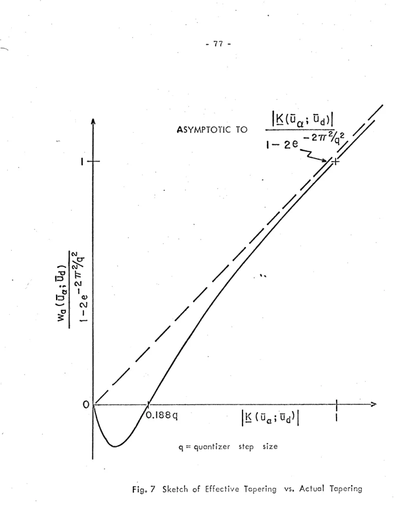
"before multiplication" by the weighting function. For uniform aperture weighting functions, the "M" function is identical for both systems. For tapered aperture weighting functions, the dominant part of the "M" function for "after-the-multiplier" quantization of data, is proportional to a linear spread function in which the tapering of the processor weighting function has been distorted. In Section IV we show that the effective tapering can be restored to a predetermined desired form by a modification of the actual tapering.

With the results on quantization available, we can make some direct comparisons between the delayed and immediate formulations of data processing. This is the subject of Section V. Here we are making comparisons of a very practical nature in the context of very general properties of the competing formulations. In the actual development of a radar system, ingenuities of design in the implemating hardware may make one formulation preferable to the other for reasons we cannot consider here.

(1)In certain cases (in particular for azimuth only processing and moderate resolution applications and where uniform aperture weighting functions are adequate) the generation of weighting functions

is simplified by the immediate formulation of data processing. (2)The immediate formulation will always require more data storage capacity than the delayed formulation by a factor ranging between 3 and 10, the higher ratios accompanying the finest

resolution requirements.

(3)The delayed formulation will always require faster summing circuits, the exact ratio depending on the number of parallel summers provided in the delayed formulation. However,. large numbers of parallel summers, become, in effect, additional data storage capacity which then reduce the relative advantage of the delayed formulation in this regard.

Because of the large quantities of data that will be required for the very fine-resolution, wide-area-coverage, non-real-time applica-tions, the advantage of the delayed formulation in data storage capacity will probably be decisive. The real-time processing applications, where resolution requirements are modest and area coverage require-ments (in terms of resolution cells to be evaluated per unit of distance traveled) are low, may be better served by the immediate formulation. This will be particularly true if large arrays of analog multipliers can be economically fabricated and the data is quantized "after-the-multiplier".

-15-II. A MODEL OF THE RADAR MAPPING PROBLEM

From the viewpoint of data-processing, the system consisting of a radar and a group of reflecting bodies is simply a stochastic "modulator", a device which modifies a given input signal in a way which is functionally dependent on the particular configuration of remote bodies, in the radar field of view during the conduct of a particular radar "observation" experiment. A sufficient radar

signal model is one which specifies this functional dependence in terms of the "size", or reflectivity of their remote bodies, their coordinates relative to the radar, and the variations of these parameters with time over the radar observation interval. No known model of radar signals purports'accomplish this task exactly, and it is likely that any model which did would be too complex for practical use.

The discussion in this thesis is concerned only with "mapping" radar observations, in particular with mappings of the earth from aircraft. Such observations are differentiated from other types by the following characteristics.

(1) The remote bodies are linear time-invariant "scatterers" of electromagnetic waves and their positions are fixed relative to each other.:

(2) The distribution of scatterers is "dense" in the scatterer space.

Extension of the model to include slowly moving isolated scatterers, e.g. terrestrial vehicles, can be accomplished but will not be

(3) Time variations in the geometry of the radar-scatterer system are completely described by the motion of the radar in a coordinate system in which the scatterers are at rest, and this motion is presumed known or measurable to arbitrary accuracy.

An appropriate model for this situation is the "dense" scatterer model used by Bar-David , extended to include certain geometric attenuation factors. In this model an elementary object called a

"point scatterer" is defined, and real scatterer configurations are modelled as simple summations of these objects. The functional dependence of the received signal on the scatterer parameters is made independent of the form of the transmitted signal by assuming linearity for the elementary radar-point-scatterer system, i. e. by assuming the existence of an impulse response description.

Let u (or u ) represent coordinates in a "scatterer space" being

x y

mapped by our radar, and let um denote a particular point in this scatterer space. Then a "point-scatterer" is defined by a function, h(t,t';u ), which is the response (at the radar's "receiving" terminals) at time t to a unit impulse transmitted at time t' when only a "unit" point scatterer is present, at the point u m, in the scatterer space. With e (t) representing the complex analytic form of the real

trans---C

mitted signal ec (t), we have

er (t;uM) - L(t, t" ur ) e (t')dt' (1)

In general, a complex function representing the received signal in complex analytic form.

17

-for the complex received signal and

el

m

t

{-r

m }

for the real received signal- from a unit point scatterer at um When a collection of scatterers is present in the scatterer space, the complex received signal is taken as

Er (t)=

j

-mer(t; r) + n(t)

(2)

m where

Yt a complex reflection coefficinet for the -M th

m point scatterer

n(t)= an arbitrary additive noise process in complex analytic form.

In the limit of a continuous distribution of point scatterers in the scatterer space being observed, we generalize to {(Ux), a complex "scatterer density function" and let

The transmitted signal is "analytic", by assumption, and we will assume that h(t, t'; um ) is such that e (t; um ) retains this analytic

character. By "analytic" we mean that e (T; um) for -r = t + jc is finite over the whole half-plane where cr > 0. As is well known this implies that the real and imaginary parts of e (t; tr) are a filbert

-- r n

Transform pair and that the Fourier Transform of e r(t; uT) is zero for negative frequencies. Consequently reception of e (t;u m ) is

equivalent to reception of e (t; um).

E

(t) dux

Y()e

(t; ) + n(t)

X -r -x

(3)

: d ux / dt'

(x)

(t')h(t, t'; ux)+ n(t)

Again the actually received real signal is

Erl (t) i = Er (t)

The central pointis that the specific form assumed for h(t, t';u ) becomes the definition of a point scatterer. _mr If we

associate a particular type of physical body with a "point scatterer", e. g. a perfectly conducting sphere, then h(t, t';um ) will be related to

the solution of a rather complex boundary value problem. A more practical approach is to assume an h(t, t'; um ) with a simple form,

which obeys the known energy and propagation velocity constraints on electromagnetic radiation, and adopt the convention that for every E (t) there exists a T(Ux) which could have generated it according to Eq. 3. The defined purpose of our radar will be to extract a re-presentation of x \ux) 2 from E (t); the interpretation of |UxF) 2 in terms of actual reflecting bodies is then a separate problem which we will not consider. As a practical matter, the interpretation problem is always solved empirically, i.e. by testing.

Let ud represent the coordinates of a point in "map space", i.e. the coordinate system in which the radar data processor will construct a representation of lY(ux). Let I(Ud) be a

complex map function and let I(d)\ 2 be the desired representation of Y(ux Ud) 2 _{We will consider linear operations on Er(t) of}

the form

I

(ud)

rft) (t; ud)dt (4)

in which the integral is to be evaluated for every ud point where a value of lI d) is desired. The function f (t; d) is termed the "processor weighting function". Its selection to optimize some aspect of jI(ud) |2 is a topic that has received considerable

attention. 1,6,7 Bar-David1 showed that when '(u_) and n(t) are complex normal random processes, and f(t;ud) is correctly chosen, the linear operation given in Eq. 4 yields a maximum a-posteriori probability estimate for (Ux Ud) = for all ud, and he obtained a solution for this f(t; ud). If we put Eq.3 into Eq. 4 we obtain

(u )d t (u e ( u t; u d ) (ud ) (5)

d x x- '--r d d

Or

I(ud) =duX() u r d; x) ( 6)d

and

L(Ud;

x)

= ddt e (t; r

)f

(td) (7)

is termed the radar "smoothing function". Its squared magnitude

is called the radar "spread function". We may note the "spread function",

L

-d

Ud

T

2 is an "impulse response" in the sense that a single "unit point scatterer" located at u = u has a scatterer density function representation of Y(ux) = (u-um). The "map" which would result from the radar "viewing" this "scene" is just

l"ud

u;r-The interchange of the order of integrations in Eq. 5 which allows us to write Eqs. 6 and 7 is valid because of the linearity of the defined data processing operations. In Section IV of this thesis we will be concerned with the effect that quantizing E (t) has on

2

|u1

2

and this interchange of order of integration will no longer be valid. However, we will want to compare radar operation in the quantized case to the linear model of Eqs. 6 and 7. This will be done by devising a representation of radar operation in which 'T(ux) is a random process.

As a practical matter, Eq. 7 is the usual basis for selecting the processor weighting function, f (t; ud), rather than some theoretical

- 21

-a sh-arply pe-aked ch-ar-acter ne-ar ud = u and falls off to very

small values outside the small region occupied by this peak, we have an intuitive feeling that the radar maps produced will be of

high "quality", i. e. will show fine details in the structure of

i(ux)

1

2 _{with good fidelity. The more sharply peaked the spread}

function, and the lower the skirts, or "sidelobes", the better the expected "quality" of the radar map. Quantitative measures of radar mapping quality are usually defined in terms of the spread function, and we will have occasion to discuss these more fully in

subsequent sections. For the present we need only the well known fact that the weighting functions, f (t; ud), which produce the most desirable spread functions have arguments (i. e. phase functions) which are equal to the argument of er (t; d) and have magnitude

functions which are similar to e (t;ud) (i.e. f(t; ud)l wvill have

appreciable value only where ler(t; ud) has appreciable value) but not niecessarily exactly the same. The phase matching condition is essential to producing a sharp central peak in the spread function.

The m~agnitude of the processor weighting is often adjusted empirically to produce a desirable shape in the spread function in the region out-side the central peak. Of course the result actually obtained depends on both f(t;ud) and e (t;u) but the freedom to select e (t; um) will be

limited by practical design poblms and the physics of the situation. limited by practical design problems and the physics of the situation.

the major portion of its extent in t, the processor is said to be

"matche d". +

The foregbing radar mapping model may be called a "temporal" model, since the desired processing operations are defined as integrations on time, t, and the received radar signal E (t) is obtained as a function of the single independent

-r

variable, t. There is, however, an alternate model which we

shall term "spatial", which will lead us to better ways of synthesizing the processor weighting functions and to simpler processing. In this section we will give a general development of the spatial model and illustrate it by an idealized example. In Appendix A we give an example using a more realistic geometry.

Consider the unit-point-scatterer impulse response function, h(t, t';u ). _m The simplest form that this function can take, consistant with a constant radiation propagation velocity5 and with conservation

of energy, is an impulse delayed by the round-trip propagation time,

Once e (t; um) is specified, there is, of course, only limited freedom

-r m

in shaping the spread function through choice of f(t; ud).

+It is well known that a matched processor maximizes Xne expectatihn cQ-e ratb of I(ud)( to N(ud)j when n(t) is "white noise"

23

-attenuated by the spherical-wave law and amplified by the directional characteristics of the radar antenna, i.e.

h(t, t';u )

6

tt-t-

x(t)4rmx(t'))

(8)

m mx mx

where xR (t) distance from the radar to the point scatterer at point u at time t

g (t) = antenna "gain", relative to unity for the antenna

orientation and position at time t, in the direction of the point u

m

c = propagation velocity

and 6(t) = the unit impulse (Dirac delta function) at t = 0

If the radar antenna follows a known (or measurable) path in the fixed coordinate system containing the scatterer space, and its

velocity along that path is newr zero, then a one-to-one correspondence can be made between distance, S, along the path and time, t. We can then write S = S(t) and we can always find a form for mx(t) like

mx ,R _mx (t) = R mx(S(t))_mx Similarly

gm

(t ) G m(S( t)) rm (t ) mx

This particular model for h(t, t'; u ) is real. Hence we shall drop m

Now, if we define a "propagation distance", R, by

R(t)

_{2 (t}

(t_ Tn

_n)

where T = an arbitrary reference time we can write for h(t, t'; um)

h(t, t';um)

=

i (u(t), u

a ( t ' )

;

u

)

(9)

where

unit) = (R(t), S(t))

and

i(u

a

_,

ua u

_a

m )

_m

G(S)G

m(S')6[-

(R-R'-

_(gA

n

_a

RrnS')

(9A

with u = (R, S) u ' = (R',S')

We have obtained the spatial function i(uu ';1u ) for a special a 0a m

h(t, t'; u) but the process is by no means limited to this special choice of h(t, t';u ). Furthermore, the i we have obtained is dependent upon the particular choice made for the spatial variables

R and S, and indeed these need not be limited to two. In general, if'we are given an i(u_a , u ';u ) function and a one-to-one mapping from "t" onto a one dimensional subset of the ua, space, i.e.

-

25-Eq. 9, then we can define a spatial radar model by

vr( a; um) _/i(ua,u _a (t'); _{u m )e c} (t')dt_' (10)

v (u~)

-

Y

(u)

v

r(ua;

+

x)

2v (u)

( 1)

I(d)

-

du Vr(Ua)K (ua; ud)

(12)

where again we desire to have | I'(d) 12 be a representation of

Y(um=

ud). We'now inquire as to the conditions under which I '(ud) 2 will be equivalent to I I(ud)

12;

under what conditions the actually received radar signal, E (t), can be

used to obtain V (u ); and what are the advantages of processing according to the spatial model rather than the temporal model.

The questions of equivalence betweenlI'(ud)12 and 1k(ud) 2 and construction of V (u

)

from E (t) are easier to answer in

-r a. -r

reverse. That is, simple comparison of Eqs. 9, 10, and 11 with Eqs. 3 and 4 shows that

For completeness we introduce a spatial noise process, i(ua), which should correspond in some sense to n(t), the temporal noise process in Eq. 2. The effects due to this spatial noise process will be carried along in the equations but we will temporarily ignore the noise in

discussing the relationship between the temporal and spatial models of the radar signals. We will return to noise processes at the end of this section.

E (t)= V (u (t)) -r

r

r(t;u) =

vr(ua (t);Tr)

and I(ud) = fdt Vr(U (t)) K

(u

(t); (13)

provided

n(t) =

(u

a

(t))

and

f(t;u)

=

K(u

(t);u

)

- d - d

(This last condition is certainly easy to meet. It merely requires that K(ua; u d) bear the same relationship to v (u a ; u = ud) as

f(t;ud) bears to e (t;m _{dr m} = ud) _d i.e. identical argument and "similar"

magnitude.) Hence given Vr (u) and the ua = u (t) curve we could certainly construct E (t) but the reverse process is not assured,

-r

a-priori. But E (t) is, in fact, a sampling of V (ua) over the u

-r -- r a

space, specifically at the points ua = ua (t). Then a set of conditions

under which E (t) suffices for the construction of V (u_{r -r} a_a.) is well

known, namely that V (ua ) be strictly "bandlimited" as a function

of each u coordinate, and that the u = ui (t) points be regularly

a a. a

distributed over the ua space at intervals along each coordinate that are less than the inverse of the bandwidth associated with that coordinate. Similarly it can be shown that I(Ud) as given by Eq. 13

27

-will be strictly proportional to I'(ud) if both V (ua(t)) and K(u a (t);ud) are adequate samplings of V (ua) and K(u ;Ud

)

This last statement can be paraphrased in terms of smoothing functions, i.e.

(ud) fdu i (ux)(d;U d ) + (ud) (14)

where

rI

UdiTm) =

af r

T a(; a m)$ (ua.; ud) (14A)

and

N' (ud) = du a a (uKu a ud )

while repeating Eq. 6

I(u d ) = f^duX (~x)(F ;-- -+lTU ) d (6)

and comparing Eqs. 7 and 13

-(u

d;

m) = dt v (u (t); U )K:(u a (t); ud)

Hence I'(Ud) and I (ud ) are proportional if F(ud; u) and

r,'(ud;U

)

are

proportional for every

um

point

where

(u) fO;

-- d m - m

and the latter will be the case if both v (ua (t); u) and K(u a (t); u d )

are adequate samplings of v (ua;um )and K(u'ud ) respectively, for

every um point which is "illuminated" by the radar.

All of the foregoing suggests that the roles of the spatial model and the temporal model should be reversed, i. e. we should regard

the spatial model, and in particular i(u, ua'; ud), as fundamental and the temporal functions, in particular h(t, t';ud) as derived quantities pertinent to a particular radar observation " experiment". In view of the arbitrariness cf i(ua , u

t';

u ), it will be impossible

to justify such a viewpoint in a completely general context.- How-ever, for particular h(t, t';u m) and i(u ,ua ';u ) combinations, a

simple test for the validity of i as a continuous function can be given; namely "does Eq. 9 hold for every sampling of the u space obtained from ua = un (t) by independent linear displacements of the u (t) coordinates relative to t, i.e. is the connection between i and

h valid for the sampling given by

R= R(t + T)

u

(t)

(14 B)

a

T S =s(t)

for every T?" As a minimum, this will require that u(t) be a one-to-one mapping from t onto a one-dimensional subset of the u space.

We will henceforth refer to the ua space (sometimes denoted

up)

as the "sinal space". The functions v (a ;u ) and K (u ;

d)

up s "ina pae -r a' m CL d are then mappings from scatterer space into signal space, and front signal space into map space respectively. For most of the rest of this theses we can regard these as "given" functions. Their joint product and summation over the signal space by Eq. 14 defines

29

-the "smoothing function," F, of -the radar, which in turn provides

a connection between the "scatterer density function" Y(u ), and its complex-map representation I(Ud), via Eq. 14. The mapping u = u (t), with a suitable interpolation rule, provides the means of converting the actually received radar signal E (t) to the spatial

-r

signal Vr(u). (The interpolation can be actual, as is provided by the CRT spot size in a "signal film" recorder, or implied as in a computer integration algorithm. ) We assume that the ua= a (t) mapping meets the minimum sampling requirements on v (u

;u

m )

(and hence on V

(U

) and K(u ; ud)) and hence we can drop the -r a. - a d

primes which distinguish the smoothing (-) and (I) functions in the temporal and spatial models.

The foregoing general development can now be applied to a specific radar mapping problem. Here we will consider only an idealized geometry, which does, however, preserves the essence of the problem. Appendix A gives the extension to a realistic geometry.

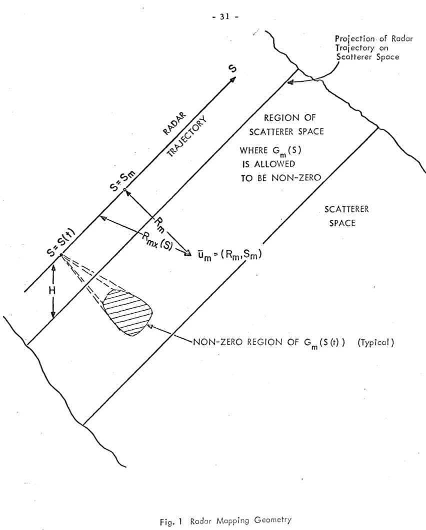
First let us stipulate a scatterer space confined to a plane and a radar trajectory which is a straight line at a constant height, H, above this plane. Let S be distance along this trajectory and the radar (to be precise the "phase-center" of the radar antenna) travels along the trajectory at the constant speed U . Take the scatterer

o

space coordinates, i.e, the components of u at the scatterer m

point "m", to be R and S where R is the length of the perpendicular from "m" to the radar trajectory, and S is

m

the value of S where this perpendicular meets the radar

trajectory. Then

Rmx(S) Rm + (S-S ) (15)

and the geometry is shown in Fig. 1. This will be recognized as an idealization of the usual synthetic aperture geometry for "broadside" operation.

For the transmitted signal, take a complex pulse train of the form

-_ ;*~

(

t-

Tn) w_o(t- Tn)

e

(t) = a(t-T )e ej (16)

n where

a(p) = a pulse amplitude function, non-zero over an interval 0 <1¢<T << T - T

.-- p n+l n

Tn T-1 .. = a set of time instants, equally spaced on t.

@(F) = a non-linear phase modulation function. 0o = the carrier "frequency" (in radian measure)

-31-'

Projection of Radar

Trajectory on

Scatterer Space

<>'~'/

/

REGION OF

t/7

/O

SCATTERER SPACE

/~:

/9c

/

WHERE G

m

(S)

IS ALLOWED

TO BE NON-ZERO

SCATTERER

SPACE

/

''

5,

um -

( R mS m )

/-NNON-ZERO REGION OF Gm (S

(t))

(Typical)

Starting each pulse at a given phase can be regarded. as

equivalent to "coherent detection" of the received signal. By limiting the extent of the signal space in the R dimension, we can specify ua (t) as the following one-to-one mapping from t onto

the one-dimensional sublset of signal space shown in Fig. 2:

R(t) c (t-T ): T < t<T R = 2 n n - n+l

(0u

(t) -S) Ut' allt(17)

a

t

S(t)

=

U t; all t

0

Hence 0 < R < (Tn - T n ), - < S < defines a "strip" in

signal space over which v (u ;um) is sampled.

Combining ec(t) from Eq. 16. the ua(t) mapping of Eq. 17 and the i(u u ':u ) function of Eq. 9A gives for v (u ; u )

a a m --r a. m by substitution in Eq. 10 -r= ea _{d ,4,31} U _{Si 2}

-R'(S)+R

_{R '( S}

R

m

_M

(S')

2

_: a

m

L j

m

2

0 0 (17A) GO (S) G (S') m m where R'(S') = -2U (S' - S ) S < S' < S 2U n n n and S UT n o n

- 33

-·

_(O) LU <

u~~~~~

ZU

o

0

0~~~~

o .--F-~~~~~~~~~~~~~~~~~~~~F0

~~~~~~~~~~~C

~_l.- 0 D 4-a.

~

DL

~

~

~

~

~

~

~

~

. Iu S C~~ .Q~~~~~~~~~~~~~F_{O II o,~~~~~~~~~~~~~~~~~~~~~~~~~~~~~~~}

1:3

U-~~~~~~~~~~~ I I Z~~~~~~~~ L.~~~~~~~~~ I o: C3~~~~~~~~~~~: w~~~~~~~~ ar~~~~~~~~~~~:

This integral is of the form

_

f(xo)

f(x)

6(g(xj))

d=

x

dx X= X

where

x0 =[ g(x) = o

Finding the values of S' which cause the argument of the delta

function in Eq. 17A to go to zero is straightforward but

algebraically complex.

Sufficiently accurate solutions for most

practical applications are

2U

S ' = S

+

° [ R - R (S

on n c m

where

S < S '< S n- on n+l O<R <2 (Sn+l S o

Using G (S')

G (S) since this function varies very little over

m m

the intervals (S

n+- S

), we obtain

n+l n

-- r(Ua;u

m )

= O

(S) a

c (R - R (S

)

4 (u G(18)

ej {c (R-Rr(S))eJX (R-R (S))

where

X

-

c - "wavelength" of the carrier and the sum on n

-35

-has disappeared because each term of the sum defines v (Ua;U ) over a single rectangle in signal space (the rectangle (S nl-S) _{n+l n} x ₂ (T _n+ - Tn)) and the v (U; u ) so

1 --r a

obtained is continuous across the rectangle boundaries.

Having found vr (u; uM), our model is essentially complete. There remains only the task of specifying the T instants (or the Sn positions) so that ua (t) is an adequate sampling of signal

space, for every um point which is illuminated by the radar. But vr (ua;u ) will be confined to the allowed strip of signal space only if

G (S) = 0

for R _m > - T ) - R - (S + ) R S))

2 Tn+l a mx m -2- mx(Sm

where S = the "azimuth aperture", i. e. the length of the a interval for which G (S) is non-zero._m

R T the "range aperture'.

a 2 p

The "bandwidth" of v (u,; ) along S, the sampled dimension, -- r x(S)

is determined by the 2(S) ej factor. The non-zero width of G (S), i. e. Sa, must be finite if we are going to map a

m a

non-zero map width (by the foregoing limits on G (S) as a function of Rm) so v (u ;u _m ) cannot be strictly "bandlimited" along S. This

is the usual dilema of sampling; so we will not belabor the point.

The "effective" bandwidth. WS, of v (ua ;

u

)

along S can easily

be shown to be W s -~ = a rad. /unit dist. The usual criterion

m

for sampling of complex waveforms is that (Sn+- Sn < The sampling requirements thus yield a set of constraints on G (S) as a function of S and R , and on the spacing of transmitted pulses.

We can now consider the question of the utility of the spatial model vs. the temporal model, at least for the example we have just given. A weighting function based on Eq. 19 for v (T

;'

m )

would have the form

.K = w( u )e

(R-R(ud)

R (S

where

w(ua;u d ) = an aperture weighting function Ud = (Rd'Sd)

Rdx(S) = J R + (S - Sd) -j 47rR(i -X)

Here the factor e has been segregated to adjust the'~patial carrier" frequency of the remainder of K along the R coordinate from 4wr/X to 4?r/Xi radians per unit distance. Loosely

37

-speaking, Xi can be regarded as the "intermediate frequency wavelength". When the proper precautions are observed+, the

-j4rR( I _ 1)

e part of K can be introduced into the signal processing before the conversion of E (t), the received temporal signal, to Vr(ua), the "received" spatial signal. The other strange

4r

factor, e , is introduced to bring the average spatial frequency of K as a function of Rd to zero. This is permissable since the only effect is to shift the phase of I(ud) as a function Rd. while only \I(d)1t

is of interest in the final result.

+

-j47rR ( i - X) +j(t-Tn)(o i 2

The factor e =e (where ei= 3

represents a frequency "translation" when applied to the received signal. Hence, the "proper precautions", consist of (l)insuring that the full

j(t-T ) (c -ci )

complex form of E (t)eo is available after the translation

-r

if W. is less than the bandwidth of E (t) and (2)insuring that the

"local-1 .-- r

oscillator" phase is reset to zero at each t= T instant or some equiva-n

lent operation is performed to retain pulse-to-pulse phase continuity in the received signal. Requirement (1) above may be avoided if G (S)

j(t-T,) O- i )

is such that the V (ua) constructed from E (t)e n is analytic

--r a --r

along the S coordinate in signal, ua , space. Or the "local-oscillator"

may be phase modulated as a function of S to accomplish this same purpose. As long as V (Ua ) is analytic along one coordinate in ua,

The temporal weighting function f (t; ud) which corresponds to the K(u, ; ) in Eq. 20 would be obtained by the substitution

= u (t) where u (t) is given by Eq. 17. It is fairly evident

that the two dimensional function, K, will be easier to work with in most types of physical apparatus than the one dimensional function, f. At the very least it is easier to visualize.

-The method we have used to derive v ('u; ; ), the complex spatial return signal from a point scatterer, is not unique. The more usual procedure is to visualize the construction of a "signal film" by recording successive "range traces", which are intensity

modulated by the return signal, side by side. For the simple geometry of our example either method is equally effective. How-ever, when the geometry is not so simple, in particular when the

radar trajectory is somewhat unpredicatable (although still measure-able), the method developed here provides a sound and easily applied analytical connection between a spatial signal model and its temporal counterpart. The present method also provides a model which is independent in conception from any particular implementation of

processing, but is equally applicable to all implementations.

There remains only the question of the correspondence of the noise processes n(t) and TI(ua). If n(t) is assumed to be broad-band "white-noise", as is usually done, then T_(u _{a )} should be taken

as a multidimensional "white-noise" process, i.e. having a flat broadband spectral density along every coordinate in

signal space. Then every sampling of signal space, by Eq. 14.B, will yield a statistically equivalent white noise n(t) = 1(ua (t)) .

However, it is also clear that no sampling of the signal space is "adequate" from the standpoint of the noise processes. This means that no construction of V (u) from E (.t) gives a

broad--r a -r

band ](ua) component but instead yields a V r(U) with an (ua )

component which has "bandlimited" spectral distribution, of band-width approximately equal to 27r divided by the sampling distance (in radians per unit distance) along each coordinate.

The distinction is largely academic, however. For this band-width is greater than the bandband-width of K(ua; ud ) along each coordinate

in signal space. This must be so because K(u (t);ud) is an adequate

sampling of K by assumption. Since the only use to be made of V (ua) is to "filter" it by K(u ;Ud), no significant penalty is incurred by considering the V (ua) obtained from E (t) to have a broadband "white-noise" component along every coordinate in signal space.

III. ALTERNATIVES FOR ORGANIZATION OF DATA PROCESSING In this section we will discuss the functional requirements implied by the processing equation given in Section II(Eq. 12)

I(Ud)

=

V

r

ar

a

(U

a;

Ud)

(12)

By this we mean sequences of operations which must be performed

on the received signal, E (t to obtain I(uda)

for

every ud

point of interest. There are, in fact, several alternative sequences, of which two will be discussed in detail here. We refer to these alternatives as "formulations" of the data-processing problem.

In this and succeeding sections we will assume signal space coordinate, ua, of propagation distance, R, and trajectory distance, S, as used in Section II and in the more detailed example of Appendix A. (In Appendix A, S is a "nominal-trajectory" distance.) Although

other signal space coordinates are possible, these will suffice for our purposes. We also assume a two-dimensional scatterer

space u = Rx, Sx ) (or u , or, when a particular point is to be

X ¥ y

designated, u = (R , S m)) and a two-dimensional map space of

coordinates ud =(Rd, S d ) .

The operations for obtaining | I(ud)

2

defined by the processing

equation (Eq. 12), given v (u a ;u ) (and hence by implication

KQ;U

d)) present a significant realization problem only because the -number of map points to be processed is enormous. It is generally

desired t- evaluate II(ud)2 for values of ud which correspond to an interior point of each contiguous resolvable element (or "box") in the scatterer spaced scanned by the radar. A rather ordinary