Development of the in vivo flow cytometer

(1)

Development of the In Vivo Flow Cytometer

by John P. Novak S.B. Aeronautics/Astronautics MIT 1980 S.B. Mechanical Engineering MIT 1980 S.M. Mechanical Engineering MIT 1995 S.M. Nuclear Engineering MIT 1995

SUBMITTED TO THE DEPARTMENT OF MECHANICAL ENGINEERING IN PARTIAL FULFILLMENT OF THE REQUIREMENTS FOR THE DEGREE OF

DOCTORATE OF PHILOSOPHY IN MECHANICAL ENGINEERING AT THE

MASSACHUSETTS INSTITUTE OF TECHNOLOGY

SEPTEMBER 2004

and to distribute publicly paper and electronic copies of this thesis document in whole or in part.

Signature of Author:

Department of Mechanical Engineering July 16, 2004 Certified by:

Charles Lin Assistant Professor of Biophysics Thesis Supervisor Accepted by:

Ain Sonin Chairman of Graduate Studies

C. Forbes Dewey

Professor of Mechanical Engineering

Roger Kamm MASSACHUSETTS INSIIUE Professor of Mechanical Engineering, Bioengineering

OF TECHNOLOGY

(2)

DEVELOPMENT OF THE IN VIVO FLOW CYTOMETER By

JOHN NOVAK

Submitted to the Department of Mechanical Engineering on July 16, 2004 in partial fulfillment of the

requirements for the Degree of Doctorate of Philosophy in Mechanical Engineering

ABSTRACT

An in vivo flow cytometer has been developed that allows the real-time detection and quantification of circulating cells containing fluorescent proteins or labeled with fluorochrome molecules in live animals, without the need to extract blood samples. A stationary laser beam is focused by a cylindrical lens to a slit of light that is then demagnified and focused across a blood vessel by an achromat and microscope objective. Fluorescent cells are excited one by one as they flow through the excitation laser light slit, creating a burst of fluorescence whose width is inversely proportional to their velocity. The fluorescence signal is detected through a confocal slit aperture using a photomultiplier tube. The analog signal from the photomultiplier tube is then digitized, filtered, and recorded as a function of time onto a computer. Computer programs post-process the data for the presence of cell signal, as well as various aspects of the cell signal such as height, width, and temporal location of the signal peak.

Two in vivo flow cytometers have been built: a single-slit, single-color system and a two-slit, two-color system. The single-two-slit, single-color system provides excitation at 632 nm, and the slit, color system provides excitation at 632 nm and 473 nm. The two-slit, two-color system can operate in several different modes: single-slit at 632 nm or 473 nm, double-slit at 632 nm or 473 nm, and double-slit with one excitation slit at 632 nm and the other at 473 nm. Thus far, the single-slit, single-color system has been used to study the circulation kinetics of different prostate cancer and leukemia cell lines with different metastatic potential, as well as the effect of different host environments (i.e., mouse versus rat). In addition, the device has been used to develop a new in vivo labeling method of white blood cells that does not result in significant depletion of the labeled cells, allowing for the possibility of autoimmune and transplant rejection studies. The two-slit, two-color system is being used to track two different cell populations, or one cell population labeled with two different markers, one of which can be the green fluorescent protein.

Thesis Advisor: Charles Lin

(3)

Chapter 1 Introduction: Research Problem Definition

and the Proposed Solution

The study of tumor cells circulating in the bloodstream and their ability to form secondary tumors has been an area of research focus for numerous years. The reason for this is that death due to such cancers as breast, prostate, and colon is primarily caused by

secondary tumors that metastasize from the primary tumor. However, despite the advances made in malignant tumor (i.e. cancer) research over the last several decades, many questions still remain to be answered about this medical malady. For example, it is hypothesized that the shedding of tumor cells into the circulatory system is one of the key steps in cancer metastasis, but it is not known at what stage or stages in tumor growth that this occurs'. It is also not known if the circulating tumor cell (CTC) count is

representative of metastatic potential of the tumor, and if the CTC count is indicative of tumor burden'. In addition, it remains to be discovered what correlation exists between

CTC count and the patient's (human as well as animal) response to malignant tumor

therapy (such as hyperthermia, ultrasound, and photodynamic treatment), and whether malignant tumor therapy may actually initiate or accelerate the metastasis process via an increase in the CTC count.

One of the current methods for the detection and counting of circulating tumor cells is (ex vivo) flow cytometry. This method involves the extraction of blood cells from the patient or test animal, the fluorescent labeling of specific cell populations, and the insertion of the blood cells into a flow cytometer. The standard flow cytometer, comprised of a light source (usually a laser), optics, light filters, light detectors, fluid lines, and electronics, passes the cells of the withdrawn blood sample in a single file through the light source and determines, via analysis of the fluorescent signal and the forward and orthogonally scattered light, the types and number of cells present.

Another contemporary device employed to detect and count tumor cells is a hemocytometer. The hemocytometer is a cell-counting chamber. It is comprised of a grid composed of small squares, a cover glass mounting support, and a cover glass. The cover glass is placed on top of the cover glass mounting support to create two counting

(6)

chambers. A solution created from a withdrawn blood sample and containing labeled tumor cells is introduced into the counting chambers using a pipette. The hemocytometer is placed on a microscope stage, and labeled tumor cells are selected and counted visually against the grid, located underneath the counting chambers (i.e., underneath the cover glass mounting support). Based on the number of cells counted, the number of squares of the grid occupied by the cells counted, the depth of the counting chamber, and the

volume of the blood sample withdrawn, the number of tumor cells in the blood sample is calculated.

Both of these methods do have merit in that both are sensitive and specific. However, a distinct disadvantage to both techniques is that they are invasive in that extraction of blood is required. In addition, each extraction of blood provides only a single time data point. Thus, obtaining a valid temporal population profile for an

unknown result or characterization of a process involving rapid changes in the number of circulating cells is problematic, and would require numerous blood extractions closely spaced in time. For test animals such as mice and rats, which have a limited blood volume, such biological studies would require the usage of many animals to avoid affecting their physiology (and, hence, invalidating the test results) due to excessive blood loss. However, the usage of numerous animals would then raise questions concerning host variability, again bringing into question the validity of the results. In addition, for numerous blood extractions as well as numerous hosts, and for the time delays involved between blood extraction and blood analysis, there is ample opportunity for sample contamination as well as damage to the cells of interest, resulting in erroneous data2.

Non-invasive methods such as positron emission tomography3, high-resolution magnetic resonance imaging4, intravital microscopy5, confocal imaging6_,

bioluminescence7, and two-photon imaging8 do exist, and have been used to visualize and study the different steps of tumor progression and tumor metastasis. However, even though these techniques span a wide range of spatio-temporal resolutions, none of them have been optimized for detecting quantitative changes in the number of circulating tumor cells. For example, confocal imaging can provide visual images of fluorescently labeled tumor cells flowing through a blood vessel, but counting usually must be

(7)

performed manually. For high cell velocities and/or large numbers of labeled cells, accurate cell counting is virtually impossible. The images can be viewed in slow motion after the acquisition of the data, but it can still be difficult (and fatiguing) to discern fast-moving individual cells or cells in a group. In addition, post-processing of the data requires that the images be stored during the test, resulting in extremely large computer

files. Software does exist for post-processing analysis, but is slow, difficult to use, and of limited accuracy. Finally, the acquisition of good images requires the usage of a high numerical aperture lens, limiting the depth of focus of the system and, hence, affording the possibility, except for very small diameter blood vessels, that labeled cells will pass

by out of the depth of focus of the system.

To remedy these problems, an in vivo flow cytometer has been developed with the capability to detect and count circulating fluorescently labeled cells in live, adult, fully-furred animals, without the need to extract blood samples. In addition, this technique allows for the continuous monitoring of the labeled cells of interest in one animal, and it yields quantitative information on the labeled cells without affecting the physiology of the host animal. The underlying principle of operation of the in vivo flow cytometer is confocal excitation and detection of the fluorescently labeled cells in circulation. Light from a laser is focused into a slit by a cylindrical lens and then demagnified and imaged across a blood vessel using an achromat lens and a microscope objective (see Figure 1.1). The blood vessel is chosen using another aspect of the cytometer called the transillumination section. The slit of light across the blood vessel excites fluorescent proteins within or fluorescent labels that have been attached to the circulating cells in the blood stream of which one would like to detect. The fluorescence that results when the fluorescent protein or the fluorochrome molecules are excited by the slit of laser light is gathered by the microscope objective and directed, using mirrors and dichroic beam splitters, to a mechanical slit which is confocal with the slit of laser light imaged across the blood vessel. This confocalness of the mechanical slit with the slit of laser light focused in the blood vessel provides blockage of light from sources not in the blood vessel. A photomultiplier tube directly behind the mechanical slit provides

(8)

microscope objective

fluorescently labeled cell _{blood vessel wall}

fluorescence

v photons =Milo,

aser beam

Figure 1.1 Excitation of a labeled cell by laser light slit

vessel. The analog signal from the photomultiplier tube is digitized and stored on a computer. Computer codes analyze the data for cell signal.

Fluorescent labeling of the cells to be detected with fluorochrome molecules is accomplished by intravenous injection of the fluorochrome molecules conjugated to

antibodies that specifically bind to the target cells. Alternatively, cells are labeled ex vivo and introduced into animals in adoptive transfer experiments. Fluorescent sources on the cells of interest can also be created by the transvection of a gene into the cells,

before the start of the experiment, which creates a fluorescent protein in them (such as

GFP).

Thus, this method allows for continuous acquisition of data from one animal with no need of blood extraction, eliminating the possibility of altering the physiology of the test animal due to too much blood loss, or the need to have numerous test animals

involved in the experiment. In addition, the possibility of erroneous data due to blood sample contamination or blood sample damage is completely eliminated. This technique also provides test results with minimal time delay, and no special preparation of the animal (such as the shaving of the fur of the animal) is required for data acquisition. Although this method allows for data acquisition on the cells of interest only through fluorescent tagging (since forward and orthogonally scattered light will not be able to be collected), this should not prove to be too heavy of a penalty, since the information desired can be obtained by analyzing the fluorescent signals recorded. Indeed, this

(9)

technique has already been used to examine the circulation kinetics of different prostate cancer and leukemia cell lines with different metastatic potential, as well as the affect of different host environments (i.e., mouse versus rat). In addition, the device has been used to develop a new labeling method of white blood cells that does not result in significant depletion of the labeled cells, allowing for the possibility for autoimmune and transplant rejection studies. In short, this method allows for acquisition of data (from mice and rats) which could be used to answer or help to answer many biological questions, including the above questions concerning time course of tumor cell shedding, metastatic potential of the tumor, tumor burden, and degree of correlation of CTC count with animal

responsivity to tumor therapy. If successful, this process could then be applied to human subjects in the future, although it is hoped that the data obtained from animal studies can be applied to humans as well.

In what follows, Chapter 2 gives a thorough physical description and explanation of the in vivo flow cytometers that have been built, and Chapter 3 discusses the computer codes that have been written to analyze the acquired data for cell signal. Chapter 4 discusses the various applications of the devices that has already occurred, as well as recommendations for changes to improve the in vivo flow cytometer systems and future tests to characterize the systems (i.e., find the detection limits of performance of the devices), along with more biological tests to perform.

(10)

Chapter

2 System Description

Introduction

Two in vivo flow cytometers have been designed and built. The first system is a single-slit, single-color system. The excitation wavelength is 632 nim, provided by a Helium-neon laser. This wavelength was chosen first because of its good penetrating

capability through tissue and blood, as well as its strong excitation capability of the fluorochromes DiD and PE-Cy5, to be utilized in planned experiments. In addition, this wavelength is sufficiently far from the emission wavelengths of DiD and PE-Cy5 where

fluorescent detection will take place, allowing for filtering of reflected excitation light from fluorescence light. The second system is a two-slit, two-color system, with excitation wavelengths of 473 nim and 632 nm. The 473 nim wavelength was selected because of its capability to fluorescently excite cells expressing the EGFP gene. A diode-pumped solid state diode laser provides the shorter wavelength excitation light, and a Helium-neon laser, like the first system, produces the longer wavelength excitation light. The two-slit, two-color option allows for detection of two different labeled cell

populations, as well as detection of cells possessing two different fluorescent sources. This second system can also operate as a two-slit, single color system, using either laser as the source for excitation. Operation of the system in this mode allows for accurate determination of cell velocity, since the distance between the slits and the time difference between the signal peaks can be accurately determined. Also, cell detection accuracy of the device is enhanced in this mode of operation since two voltage waveforms can be compared against one another. An acoustic optical modulator through which the laser beams are directed provides for this option of laser beam diffraction.

Both systems have three aspects to their physical construction: the

transillumination section, the fluorescent excitation section, and the detection section. The purpose of the transillumintion section is to provide visualization of the vasculature at depths of up to 100 microns on the area of the animal's body from which data is going to be acquired. This allows for selection of an appropriate blood vessel, both in type and size, as well as an appropriate location of data acquisition on the blood vessel, and

(11)

repeatability in finding the same data acquisition site. Discriminating between a vein and artery is required since there is a significant difference in the characteristics of the flow in these two types of blood vessels. Venular flow is much slower than arterial flow in general, and some cells will also slowly roll along the wall of a vein (something not found in arterial flow). Selection of a blood vessel of appropriate diameter is needed so that statistically acceptable data can be acquired in a reasonable time period, with minimal occurrence of more than one labeled cells traveling through the probe volume. Calculations indicate an arteriole approximately 30 microns in diameter will meet these requirements. Appropriate location of the data acquisition site is important to avoid overlying structures such a hair, hair follicles, melanin patches, and sebaceous glands, which will attenuate, through absorption and scattering, the excitation energy and the fluorescence energy. Repeatability in finding the same data acquisition site is required for valid temporal studies, since the flow or signal (excitation or fluorescence) at another data acquisition location can be different from the original site due to the changing influence of various physiological or environmental parameters.

The ear of the test animal is the area chosen to transilluminate. This area of the body is chosen because a significant amount of light is transmitted by the nonvasculature tissue of the ear due to its minimal thickness. Methocel 2% is used to adhere the ear of the animal to a microscope slide for transillumination and viewing. This adhesive is used to avoid irritation of the tissue, and to help match refractive indices at the surface of the ear to allow for a higher percentage of transmission of the transilluminating light into the ear tissue.

The fluorescence excitation section produces the slit of light which causes the fluorescence of the labeled cells. This section provides the excitation energy via a laser light and shapes the laser light into the appropriate dimensions using lenses and irises. The dimensions of the excitation slit are chosen such that the width of the excitation slit

is less than the diameter of the labeled cells (approximately 8 microns), and the height of the slit is comparable to the diameter of the blood vessel chosen for data acquisition. A

slit width of approximately 5 microns is used. A narrow excitation width is required so that excitation of more than one cell at a time is kept to a minimum, and that the slit of

(12)

skin to reach the blood vessel. An excitation depth of approximately 115 microns is required, equal to the maximum depth of blood vessel selection plus the radius of the blood vessel. The height of the slit is chosen to match the diameter of the blood vessel so that there is reasonable probability that all labeled cells traveling in the vessel will be excited, and that autofluorescence from nonvasculature tissue, which is a noise source, will be kept to a minimum.

The detection section determines the presence of a labeled cell through the detection of fluorescence photons. Lenses, dichroic beam splitters, and mirrors direct fluorescence photons gathered by a microscope objective through a filter and focus them onto a mechanical slit confocal with the excitation slit provided by the fluorescence excitation section. The photons passing through the slit are amplified by a PMT, which produces a triangular pulse-shaped voltage signal, indicative of a labeled cell present.

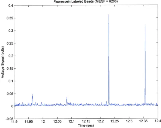
The above physical aspects of the in vivo flow cytometers are discussed further below. Included is a description of the specific components comprising each physical section of the single-slit and two-slit flow cytometer, the purpose of the components, and how the components operate together. In addition, results of sensitivity tests for the 473 nm channel of the two-slit, two-color system using fluorescently labeled beads are given and discussed.

Single-slit, Single-color System

The single-slit, single-color system is shown in Figure 2.1. As mentioned in the introduction, it is the first in vivo flow cytometer system that was built, and is comprised of a transillumination section, a fluorescent excitation section, and a detection section.

Transillumination Section

As discussed above, the purpose of the transillumination section is to

transilluminate the part of the test animal (the ear) from which data will be acquired to allow for selection of either a vein or an artery, as well as selection of a specific location on the selected blood vessel for data acquisition. The transillumination section of the single-slit, single-color system is shown in Figure 2.2. The transillumination section of the device is comprised of the sample stage, light emitting diode (LED), fiber optic cable,

(13)

In Vivo Flow Cytometer

Oscilloscope

Mirror M2

USBl device-/Ft

I'E Computer for Data Acquisition Preamplifier/Filter Three-axis Stage Achromat Lens AL3 <= f = 150 mm Optical Filter F2 Mirror M4 Mechanical

-- Slit 200 mic X 3 mm Achromat

-Lens AL1-+ ... f = 150 mm Dichroic BS1 Beam Splitter Mirror M3 Iris 11

I

Cylindrical Lens

I

f=150 mm

I-

Iris 12

F-

Iris 13 Iris 141

**N*'\T**

He-Ne Las 632 nm

K

Dichroic Beam Splitter

BS2 Achromat ~2Lens AL2 f = 30 mm - Filter F1

Mirror M1

Two Neutral 4-~~ Density Filters er

Computer for

Visual Picture Sample Stage

*

Focusing Lens LED I I 44 I Microscope Objective 40X NA=0.6

U

Fiber Optic Cable

Figure 2.1 The Single-slit, Single-color In Vivo Flow Cytometer

R

(14)

-Transillumination and Imaging Subsystem

M rror M rrca --- A ----is---- ---n -. .... .. ... ... .... M---n--- - --Achromat >Lens AL2 f = 30 mm Filter F1

F->

Sample Stage

Microscope

Dichroic Beam Splitter Objective

BS2 _{40X NA=0.6/} ₀₀ Computer for

Visual Picture

Focusing Lens

Ir\

U

LED

-T

Fiber Optic Cable

Figure 2.2 The Transillumination and Imaging Subsystem for the Single-slit, Single-color In Vivo Flow Cytometer

.9143

Ku K-A L-.41

N

S13 200mcX3 A l

---'4'111

7

(15)

microscope objective (Olympus 40X, 0.6 Numerical Aperture, infinity corrected), dichroic beam splitter BS2 (located underneath the sample stage and microscope

objective), charged-coupled-device (CCD) camera, achromat lens AL2 (focal length is 30 mm) located in front of the CCD camera, and optical filter Fl (located in front or the achromat lens).

The sample stage is where the test animal from which data will be acquired is situated. The sample stage, comprised of two separate subsystems, provides for

temperature and orientation control of the test animal. Temperature control is provided

by a heater tape (Minco HR5252R20.3L12A) wrapped around a plastic cylinder (into

which the animal is placed) and interfaced with a thermocouple (Physitemp SST-1), a variable DC regulated power supply (Physitemp MW1 22A), and a temperature controller (Physitemp TCAT2). The thermocouple provides temperature measurement of the animal's body, which is fed into the temperature controller. The temperature controller, where the desired temperature is specified, controls the on/off state of the DC power supply. The DC power supply provides electrical power to the heater tape. Thus, the DC power supply is on causing thermal energy to be created by the heater tape when the temperature measurement from the thermocouple is below the user-specified set temperature of the temperature controller.

Orientation control is provided by a three-axis linear stage, onto which is situated a custom-made rotatable plastic stage. The three-axis stage allows for translational positioning control of the animal, and the rotatable stage allows for angular orientation control of the animal. Both stages have an aperture in their center across which a microscope slide is positioned to which the test animal's ear is adhered. The two stages are interfaced via these apertures, with the rotatable stage having a piece of plexiglass tubing, which is centered around its aperture, that inserts into the aperture of the three-axis stage.

The LED (Future Electronics LXHL-MMID) provides the transillumination light. The circuit shown in Figure 2.3 adjusts the optical power output of the LED. The circuit functions by maintaining a constant voltage drop across the 1 00-ohm resistor (i.e., a constant current through the I 00-ohm resistor). This constant voltage drop is maintained

(16)

15-volt 1.5-amp Power Supply Switch LMS1587-ADJ Voltage Regulator Vin Vout Vtfd R C = 10 pIf R R = 0 to 500 ohms potentiometer = 100 ohms =43 ohms

R

- C = 10 pt

Figure 2.3 Controlling Circuit of LED

= 10 ohms

LED

i

(17)

resistor (i.e., potentiometer) increases in value, the voltage drop across the entire leg that is comprised of the 1 00-ohm resistor, the 43-ohm resistor, and the variable resistor (0 to

500 ohms) increases. Consequently, the parallel leg comprised of the 10-ohm resistor

and LED has its voltage drop (and, hence, current) increase, resulting in an increase in the power output of the LED. The capacitors in the circuit remove high frequency current

oscillations. The LED emits at a wavelength of 524 nm, which provides good contrast between blood vessels and surrounding tissue due to the high absorption of light at this wavelength by hemoglobin. The light from the LED is brought to the animal via a fiber optic cable, which, due to the ease of positioning of the fiber optic tip, allows for good illumination of the ear no matter how the animal is situated on the stage. The transmitted light through the ear enters and passes through the microscope objective, reflects off beam splitter BS2 (Omega Optical) situated below the mounting stage (the beam splitter transmits wavelengths above 600 nm and reflects those below, providing separation of the green LED light from red fluorescence emission), passes through optical filter Fl (Omega Optical) to attenuate its intensity, and is focused onto the CCD camera (Edmund Optics LCL-902C) by the 30 mm focal length achromat lens AL2 (Melles Griot). This achromat lens is located at a distance of 30 mm in front of the CCD camera so that only transilluminating light that has scattered at the focal plane of the microscope objective is in focus. The microscope objective and achromat lens together provide 6.67X

magnification. The image from the CCD camera is displayed on a computer screen (CRT), from which an appropriate blood vessel and data acquisition location are chosen. The pixel size of the CRT is 1.47 microns. The field of view of the transilluminating system is measured to be 800 microns X 1000 microns. The resolution of the

transillumination system is 0.43 microns.

The Fluorescence Excitation Section

The fluorescent excitation section is shown in Figure 2.4. It is comprised of a He-Ne laser, two neutral density wheels, four irises (I through 14), three mirrors (Ml through M3), a cylindrical lens, a mechanical slit, an achromat (ALl), two dichroic beam splitters (BS1 and BS2), and a microscope objective. The Helium-Neon laser provides the energy to fluorescently excite the labeled cell. As mentioned in the introduction, an

(18)

Fluorescent Excitation Subsystem

Mirror M2

Mechanical

-H

Slit 200 mic X 3 mm Achromat --Lens AL1 -f = 150 mm

BS1 Mirror M3 ---s ---p

---

Iris 12

I-

Iris 13

2:-:

Mirror

M1

IN

Iris

11 T

Cylindrical Lens f=150 mm Two Neutral Density Filters He-Ne Laser 632 nm S p

Sample

Iris 141

N

-,- N

N\I/

Microscope

Objective Stage

-k-

~

Theei ys - ---A- r---

---

(19)

---excitation of 632 nm was chosen for its good penetration through tissue and blood, and its efficient excitation of the fluorochromes DiD and PE-Cy5, to be used in planned experiments. Also, this wavelength is sufficiently far from the emission wavelengths of DiD and PE-Cy5 where fluorescent detection is taking place, allowing for filtering of any reflected excitation light from fluorescence light reaching the detection section. The power entering into the system from the laser is controlled by two neutral density wheels (New Focus Model 5215) situated in front of the laser, with each wheel containing five attenuating filters of different value. The collimated portion of the laser beam is obtained

by spatially filtering the laser light through an iris (iris 11). This spatial filtering is

required because the Helium-neon laser has a weak spatially incoherent component. Mirror Ml directs the laser light through iris 11. The resulting collimated beam of light is then directed, using mirror M2, into a 150 mm focal length cylindrical lens (Melles Griot), which focuses it into a slit of light onto a mechanical slit 3 mm by 200 microns (Edmund Optics R39-73 1). The iris immediately after the mechanical slit, iris 12, is used to obtain the desired length of the excitation slit at the sample stage. A 150-mm-focal-length achromat lens (ALl), situated 150 mm beyond where the mechanical slit is located, converts the slit of light into one rotated by 90 degrees and focused at the back focal plane of the microscope objective. (Both dichroics, BS1 and BS2, located in the beam path between the achromat ALl and the microscope objective, are transmissive at

632 nm. The dichroic BS1 [Omega Optical] is a short pass filter that turns off at

approximately 650 nm, transmitting light with a wavelength below 650 nm and reflecting light with a wavelength above 650 nm. The other dichroic, BS2, is a long pass filter that turns on at approximately 600 nm, reflecting light with wavelengths below 600 nm and transmitting light above 600 nm.) The laser excitation light then enters the microscope objective (the same microscope objective of the transillumination section) where it is refocused to the front focal plane of the microscope objective. The width of this slit of light at the front focal plane of the microscope objective is approximately 5 microns. This dimension is much larger than that predicted by diffraction theory and is primarily due to the underfilling of the entrance aperture of the microscope objective in the direction of the length of the slit of light at the back focal plane of the objective. This underfilling is required to provide an excitation slit of uniform intensity over a depth of

(20)

approximately 30 microns, the maximum diameter of the blood vessel that would be chosen for data acquisition. The amount of underfilling is determined by the dimension of the excitation laser light horizontal to the optical table at the entrance to the cylindrical lens, the ratio of the focal length of achromat ALl to the focal length of the cylindrical lens (which is one for this setup), and the back focal length of the microscope objective. The less the objective is filled, the more uniform will be the intensity of laser light with depth into the blood vessel. One could avoid this need of underfilling the entrance aperture of the microscope objective by using an objective of much lower numerical aperture, but this would compromise the number of fluorescence photons captured from the labeled cells. The length of this excitation slit of light is made equal to the diameter of the blood vessel chosen for data acquisition, and is adjusted using iris 12, which adjusts the vertical height of the slit created by the cylindrical lens and, hence, adjusts the width of the slit at the back focal plane of the microscope objective. The larger the vertical height of the slit passing through iris 12, the narrower the slit at the back focal plane of the objective (due to diffraction effects), the more the objective is filled in the width direction of the slit at the back focal plane, the longer the length of the excitation slit at the blood vessel. The position and orientation of the blood vessel from which data is to be acquired is adjusted by translation and rotation of the sample stage so that the data acquisition point is intersected by the laser slit, with the 5 micron dimension in the direction of blood flow, and the longer dimension spanning the diameter of the blood vessel. The power of the He-Ne laser at the sample stage is approximately 600 microwatts.

Detection Section

The detection section is shown in Figure 2.5. It is comprised of the sampling stage, microscope objective, two dichroic beamsplitters (BSI and BS2), two mirrors (M3 and M4), an optical filter (F2), an achromat lens (AL3), a mechanical slit attached to a three-axis stage, a PMT interfaced with a preamplifier and electronic filter, a USB data acquisition device, a computer (with accompanying data acquisition software), and an oscilloscope. The microscope objective in the detection section is used to gather the fluorescence photons originating at the sample stage. Calculations indicate that for

(21)

Detection Subsystem

Oscilloscope USB device P omputer for Data Acquisition Preamplifier/Filter Three-axis Stage Achromat Lens AL3 <~~ f = 150 mm Optical Filter F2 -Mirror M4 Mechanical Slit 200 mic X 3 mm ANr", n Dichroic BS1 Beam Splitter

Mirror N

Iris 14j

F->**

Microscope

Objective Sample Stage

Lens

A*

0

Cy

n ric, , Ae- ... ns....

(22)

isotopic emission of fluorescence photons, approximately ten percent are captured by the microscope objective.

NA micro=cope 0.6 -> sin(m.) = 0.6 => 0. = 36.87

0max = half angle of acceptance cone of microscope objective r = 2.50mm (working distance of the microscope objective)

y = 2.50mm -sin(90' - 36.87') = 2.00mm

A = area of photonemissionsphere intercepted by numerical aperture of microscope objective

2

r -y

A =2-)fr dy = dy

Surface area of sphere = 4 -)r - r2

-r1 1

Percentage ofphotons captured = x 100%= - xl00% = -x 100% =10%

4-7-r 4-r 10

(The actual percentage captured is slightly (although virtually negligible) less than this because emission of photons takes place off the axial centerline of the microscope objective.) These captured photons are channeled by the microscope objective down to dichroic BS2 located below the sampling stage. This dichroic is transmissive to the captured photons. (As mentioned in the previous section, this dichroic transmits light above 600 nm and reflects light below this wavelength). Consequently these photons continue to the mirror below the sampling stage, mirror M3, and are redirected by this mirror to a second dichroic beam splitter, BS2. This second dichroic is not transmissive to the captured photons (this dichroic transmits below and reflects above 650 nm) and, consequently, reflects the fluorescence photons. The captured photons are redirected by this second dichroic to another mirror, mirror M4, which directs them into the leg of the experimental setup where the detector is located. Here, to remove a large percentage of the extraneous light (such as reflected laser light, stray light from the environment, and autofluorescent light), the photons travel through an optical filter (F2) that heavily

attenuates light below 650 nm and above 700 nm. This filtered light is then focused by a 150-mm-focal-length achromat lens (AL3) onto a 200 micron by 3 mm mechanical slit, which is confocal with the slit of laser light spanning the blood vessel. A Hamamatsu R3896 photomultiplier tube with extended red sensitivity situated directly behind the mechanical slit is used to detect the fluorescence signal. The photomultiplier tube

(23)

converts the photons into a current and then amplifies the current. A Hamamatsu C6271 high voltage power supply socket converts this amplified current to a voltage, and then electronically lowpass filters the voltage signal (bandpass region of the electrical filter is

from DC to 10 kHz).

The spectral response of the R3896 (i.e., the current produced by the

photomultiplier tube as a function of wavelength) indicates that for the bandpass region of the optical filter in front of the detector (650 nm to 700 un), the photomultiplier tube produces approximately 62 mA of current for each watt of light power striking the cathode of the device. The amplification of the resulting current, contingent upon the acceleration voltage between the electron multiplying stages of the photomultiplier tube,

is a gain of 1X106. (The electron multiplying stages add electrons to the original pool of

electrons created by the fluorescence photons, enhancing the original current created by the photons. An acceleration voltage of 750 volts between the electron multiplying stages is used during data acquisition.) This amplified current is then converted to a voltage with a conversion ratio of 0.3 volts per microamp of current. Thus, the resulting output voltage from the PMT/socket device is given by the equation

V = (0.3VIpA)- (1000pA ImA)- (IXI06)- (62mA 1W)- (Pigh,). Maximum output voltage of the PMT/socket device is 10 volts.

The analog voltage signal from the PMT/socket device is fed into a USB device (Data Translation DT 9804). This USB device is an analog-to-digital converter which can sample the analog voltage signal, brought in by a BNC coaxial cable from the PMT/socket device, at a frequency up to 100 kHz. The digitizer in the device (which converts the analog signal to digital) has 32-bit resolution for the voltage range -10 volts to +10 volt. Consequently, the incoming voltage signal is digitized with a 0.3 millivolt resolution. Software on the computer allows this digitized voltage signal to be fed into a computer for storage and analysis.

The data acquisition software on the computer that has been or is presently being used to acquire and store the voltage signal from the USB device was obtained from the web free of charge (URL address is

http://www.datatranslation.com/support/results3_all.asp). The first data acquisition software used on the computer is called Scope. This software allows the user to set the

(24)

sampling rate (up to the maximum value capable of the USB device), as well as specify the location of storage of the data on the computer. However, the software does not allow for real-time processing of the data, only post-processing, after completion of the experiment. Consequently, this software was ultimately replaced by software that did allow for real-time processing. This software is called DT Measure Foundry, and is a more advanced version of Scope. In addition to being able to specify sampling

frequencies and file storage location, this software allows the user to write their own code within the data acquisition program so that the data can be processed during the

experiment.

Analysis of the digitized voltage signal involves smoothing of the voltage trace to remove the high frequency components of the trace, and then analyzing the smoothed data for signal (i.e., for the presence of fluorescently labeled cells). When Scope was the data acquisition software being used, the digitized raw data were stored during the experiment, and then smoothed at a later time after completion of the experiment. The disadvantage of this approach (of acquiring raw data at the sampling frequency and then performing post-processing smoothing), was that large data files needed to be stored. The raw data file and the smoothed raw data file, despite being binary files, were tens of megabytes in size. In addition, the smoothed data file, containing such a large number of points (6 million for one minute of data acquisition at 100 kHz) required tens of minutes of computer time to analyze for signal. To remedy these computer file storage problems, as well as expedite the analysis of smoothed data for signal, it was decided to smooth the sampled data during the data acquisition process (i.e., during the experiment), and to save only intermittent points of the smoothed data, equally spaced in time.

Since the maximum cell velocity expected was 5 mm/sec, and the slit width was 5

microns, the Nyquist sampling theorem indicated that approximately 2000 data points per second (time spacing of 5X104 seconds) needed to be saved. However, before this step was implemented, it was decided to verify that similar labeled cell counting results would be obtained. To this end, numerical tests were performed on data from nine different experiments.

Six data traces acquired at a sampling frequency of 50 kHz, three having a very high cell count and three having a low cell count, and three data traces acquired at a

(25)

sampling rate of 100 kHz with a low cell count, were chosen as test cases because of their difference in cell count as well as sampling frequency. The results of the offline

smoothing/counting process with no point decimation for each of these traces were as

follows:

Run Sampling Number of Time Length of Cell Length of Time

Number Frequency Points Used in Data Count Required to

(kHz) Averaging Acquisition Complete Cell

Process (sec) Count (sec)

1 50 50 60 2880 410 2 50 50 60 2648 360 3 50 50 60 2511 480 4 50 50 60 62 42 5 50 50 60 60 30 6 50 50 60 61 35 1 100 100 60 47 105 2 100 100 60 59 80 3 100 100 60 55 110

(As mentioned in the introduction chapter, the code that performs the post-processing smoothing is called binarysmoothingfile.m, and the codes that perform the cell counting are binaryreadingcellcountingnewJohn.m and

analysis8_newmod54_linearMFScope.m. They are discussed in detail in the next chapter.) Next, the computer code below, to be inserted into DT Measure Foundry for real time smoothing and point decimation, was written. The code allows for specification of the number of points to use in the smoothing process (nsm), as well as the amount of point decimation desired (jump). In the code below, the number of points to use in the smoothing process is chosen to be 100, and the amount of point decimation is chosen to be 24 (i.e., save 1 smoothed point in 25). The parameter p5025 is the row vector

containing the raw data points to be smoothed, pp5025 is the column vector of the raw data points obtained by transposing the row vector p5025, and g5025 is the column vector containing every 25h smoothed point

jump = 25

(26)

numberofloops = (length(p5025)/jump) - (nsm/jump) + 1 pp5025 = p5025' for j = 1:1:numberofloops lower = (((j-1)*(jump)) + 1) upper = (((j-1)*(jump)) + 1) + (nsm-1) g5025(j) = mean(pp5025(lower:upper)) end

DT Measure Foundry allows specification of the size of the vector p5025. This enables the user to control how many raw data points are smoothed and decimated at one time. This is important since computer speed is affected by this number. Too few points results in too much time used in transferring data, too many points results in too much time required for the code to execute. Computer performance appears optimal for a vector size of 2000.

Thus the row vector p5025 containing 2000 points was continually fed into the code, and the column vector g5025 was continually fed into a file, until all the data points of the data trace being smoothed and reduced in size had been processed by the above code. The smoothed/decimated file was then analyzed for cell signal. The results of this process applied to the above nine data traces is shown below. Included are the cell count and time required for cell counting for the original size file and the reduced size file, and the percentage difference in cell count and cell counting time between the original size file and the reduced size file for each trace

Run Sampling Original Reduced Percentage Original Reduced Percentage

Number Frequency Size Size Difference Time Time of

(kHz) File File Cell in Cell Required Required Original

Cell Count Count to to Cell Count

Count Complete Complete Time

Cell Cell Count Count (sec) (sec) 1 50 2880 2809 2.46 410 13 3.17 2 50 2648 2595 2.00 360 13 3.61 3 50 2511 2428 3.31 480 12 2.5 4 50 62 60 3.23 42 2 4.76 5 50 60 60 0 30 2 6.67

(27)

6 50 61 60 1.64 35 2 5.71

1 100 47 47 0 105 2 1.90

2 100 59 58 1.69 80 2 2.5

3 100 55 55 0 110 2 1.82

As one can see by inspection of the results, the agreement in cell count between the original size file and the reduced size file was excellent. In addition, the cell counting process for the reduced size file required only several seconds to complete for all the data traces. Thus it was decided to do real time smoothing and file size reduction (i.e., point decimation).

Therefore, data from the PMT/socket assembly fed into the USB analog-to-digital device would be transferred from the USB device to the smoothing/decimation computer code in blocks of 2000 points at a time via the software DT Measure Foundry. The data would be averaged and every 2 0th point would be stored into the column matrix g5025.

(Every 2 0th point instead of every _{2 5}th point would be saved to further enhance agreement

in cell count between the original size smoothed file and the reduced size smoothed file. The time penalty would be minimal.) The smoothed data in the g5025 column matrix would then be transferred to a dcf file (i.e., a specially formatted binary file that DT Measure Foundry or Scope can open and read), as well as displayed by DT Measure Foundry on the computer monitor. This reduced size file would be analyzed at a later time for cell signal using the codes binaryreadingcellcountingnewJohn.m and analysis8_newmod54_linearMFScope.m.

Alignment Procedure

Proper alignment of the components of the experimental setup is imperative for good performance by the single-slit, single-color in vivo flow cytometer, since the fluorescence signal from the labeled cells is minimal in power in comparison to the noise sources. Environmental light, laser excitation light, autofluorescent light are noise

sources that are all orders of magnitude larger than the fluorescent signal attempting to be detected. Therefore, precise alignment of the parts comprising the cytometer is necessary to achieve maximum excitation of the fluorescence molecules labeling the cells, as well

(28)

as maximum capture of the fluorescence photons from the labeled cells, and maximum attenuation of the light from noise sources. To this end, the following procedure was followed in aligning the single-slit, single-color in vivo flow cytometer:

1) The 30-mm-focal-length achromat lens (AL2) was secured into threaded tubing to

be attached to the CCD camera. The achromat was attempted to be positioned in the tubing such that, when the tubing was attached to the camera, the achromat would be located its focal length (i.e., 30 mm) in front of the camera. The tubing

was attached to the CCD camera. The output of the CCD camera was fed into a television screen. The CCD camera was pointed at a distant object and the image viewed on the television screen to which the CCD was attached. Since the object was a long distance from the camera, only parallel or quasi-parallel rays from the object would enter the camera. Consequently, if the achromat was its focal length in front of the camera, the image on the television screen of the distant object should be in focus. The image was viewed and, if blurry, the achromat was repositioned. This repositioning of the achromat lens continued until the distant object being viewed was in focus. Once the achromat AL2 was properly

positioned, the filter Fl was positioned in front of the achromat and secured into the threaded tubing.

2) The threaded tubing containing the achromat lens (AL2) and optical filter (F1) and interfaced with the CCD camera was then interfaced to the side of the structure underneath the sample stage holding the microscope objective and the dichroic beam splitter BS2. This resulted in the camera and achromat being precisely positioned along the horizontal axis of the support structure underneath the sample stage. The microscope objective did not required alignment because it was threaded into the support structure, which held it securely along the vertical axis (of the support structure).

3) A microscope slide with a dirty top surface was placed on the sample stage, and

the green LED was activated. The image of the top surface of the microscope slide provided by the microscope objective, achromat lens AL2, and CCD camera was viewed on the television screen to which the camera was interfaced. If the image of the top surface of the microscope slide was not in focus, it was bought into focus by vertical movement of the sample stage upon which the microscope slide was situated. Thus, since only parallel light from the microscope slide was focused onto the detector of the CCD camera, the top surface of the microscope slide was positioned at the focal plane of the microscope objective. (The focal plane of the microscope objective is the desired location for fluorescent excitation since it results in the gathered fluorescence photons becoming collimated after being collected by the microscope objective.)

4) The dichroic beam splitter underneath the sample stage, BS2, was positioned such that the image of the top surface of the microscope slide was centered on the

(29)

television screen.

5) Iris I1 was positioned between mirrors Ml and M2, and irises 12 and 13 were

positioned between mirrors M2 and M3. The aperture of the irises was positioned three inches above the optical table. A beam height of three inches was chosen

since this was the center height of the mounted components that would be placed in the laser light path.

6) The Helium-Neon laser was activated. Using the support upon which the laser is

situated, and mirrors MI and M2 (see Figure 2.1), the beam of the laser was directed through the aperture of the irises. Iris Il was closed down to allow only the collimated core of the laser beam to pass. Thus, a laser beam parallel to the surface of the optical table and having a height of three inches above the optical table was obtained.

7) Iris 14 was attached to the support structure (holding the camera, achromat AL2,

the microscope objective, and the dichroic beam splitter BS2) at its bottom port. Iris 14 was closed down to a small aperture yielding an opening centered in the middle of the port and, hence, centered about the vertical axis of the support structure.

8) Mirror M3, the mirror underneath the sample stage and support structure, was put

into place. The dichroic beam splitter BS 1 was positioned at a 450 degree angle in front of mirror M3. This mirror was then adjusted such that the He-Ne laser light struck the mirror at its center, and was redirected through the aperture formed by iris 14. The television screen displaying the output of the CCD camera was viewed. If the laser light was perpendicularly striking the microscope slide, the image of the reflection of the laser light off the top and bottom surface of the microscope slide would coincide with one another. (The dichroic beam splitter BS2 is slightly reflective at 632 nm, allowing one to view both of these

reflections. The reflection off the top surface of the microscope slide is a sharp circle of light while that off the bottom surface is a larger, diffuse, out-of-focus circle of light.) If the two reflections did not coincide, then mirror M3 had to be readjusted for orientation and position. This adjustment of mirror M3 had to continue until the laser beam was striking the center of mirror M3, traveling through the aperture of iris 14, and perpendicularly striking the microscope slide.

9) A 150-mm-focal-length achromat (achromat lens ALl) was secured into threaded

tubing. Also, a 150-mm-focal-length cylindrical lens was secured into threaded tubing. With the cylindrical lens positioned in front of the achromat (i.e., the laser light entered the cylindrical lens first), both pieces of tubing were placed through tubing rings attached to the optical table which elevated the center of the lenses three inches off the table (hence, the laser light was traveling down the axial axis of the lenses). The two pieces of tubing were slid back and forth relative to one another until the image formed after the achromat was a slit of light in focus at

(30)

expected, the distance between the two lenses was 300 mm, the sum of the focal length of each lens.) The two pieces of tubing were then secured together.

10) The two pieces of tubing were then slid towards the dichroic BS 1. Viewing the

television screen displaying the CCD camera output, a position was found which yielded a focused slit rotated 900 from the one formed in step (8), with parallel light in one direction. (That light was parallel in one of the directions of the slit could be verified by moving the sampling stage vertically and seeing that one of the dimensions of the slit stayed constant.) This meant that the 150-mm-focal-length achromat ALl was now positioned 150 mm from the back focal plane of the microscope objective.

11) The tubing containing the cylindrical lens and achromat ALl were secured in the

tubing rings through which they were slid. They were then detached from one another. A mechanical slit 200 microns by 3 mm was placed 150 mm beyond the cylindrical lens (at the point of sharpest focus of the slit of light formed by the cylindrical lens). This mechanical slit sharply defined the dimensions of the slit of light formed by the cylindrical lens. (The slit of light formed by the cylindrical lens was the object that was imaged by the achromat ALl at the back focal plane of the microscope objective in step (10).) Iris 12 was repositioned immediately after the mechanical slit to provide a means of controlling the length of the excitation slit at the test sample stage.

12) The mechanical slit in the detector leg was secured to a three-axis stage.

13) The achromat AL3 in the detector leg was secured into threaded tubing. The

threaded tubing was slid into tubing rings situated in front of the mechanical slit attached to the three-axis stage. The tubing rings allowed for the sliding along the axial axis of the tubing.

14) An iris was secured to the front and back of the threaded tubing. Both irises were closed down to small apertures.

15) The slit of light formed at the sample stage was partially reflected from the top

surface of the microscope slide and imaged to the detector leg. The mirror in the detector leg, M4, was positioned such that the slit of light passed through the aperture of both irises. (This would yield maximum collection by the achromat AL3 of the fluorescence photons originating at the sample stage.)

16) The irises were removed from the tubing. The tubing with the achromat was slid

back and forth until the sharpest image of the light slit from the sample stage formed at the plane of the mechanical slit. The tubing was secured in place.

17) The mechanical slit (in the detector leg) was repositioned such that the light slit

passed through the mechanical slit. Thus, the mechanical slit in the detector leg was now confocal with the slit of light formed at the sample stage.

(31)

18) The bandpass filter F2, used to reduce or eliminate light noise sources, was

secured into the tubing containing achromat AL3. The filter was placed in front of the achromat (i.e., the light entering the threaded tubing to be collected by the achromat and focused onto the mechanical slit first passed through the bandpass filter) to avoid compromising the focusing of the light by the achromat.

19) The PMT was placed immediately behind the mechanical slit to maximize the

collection by the detector of the photons passing through the mechanical slit, as well as to prevent extraneous light from entering the detector from the side.

Once the system was aligned, data acquisition using the device was begun. The experiments that were performed and the results obtained are discussed in the last chapter. Figure 2.6, shows the axial response curve of the slit,

single-Tn 2- 1.8- 1.6- 1.4- 1.2-0.8 0.6- 0.4-02 0--20 -150 -100 -50 0 50

Vertical Location Relative to Location of Sharpest Focus (microns)

100

Figure 2.6 Axial response curve of single-slit, single-color system

color system after alignment, obtained by reflecting the excitation laser light off the top surface of a microscope slide situated on the sample stage, and replacing the optical filter F2 in front of the PMT with a slightly less attenuating filter to allow the reflected laser light to reach the detector. The microscope slide was moved from -190 microns below the plane of focus to +100 microns above the plane of focus. The curve obtained shows

-.. .... .. ------. ...-- --- - - ----. --- ... - - - - -

---- -

-

----... .. . .. ... ... --- --- ----.... ... ... ... ...... / ... ..

(32)

that the laser light intensity of the excitation slit is fairly uniform for vertical lengths up to 40 microns, with the light intensity at the upper and lower edges at 75% of the peak excitation intensity at the plane of focus. The asymmetry of the curve is probably due to aberrations from the optics of the fluorescent excitation section.

Two-slit, Two-color System

The two-slit, two-color system is a more advanced version of the single-slit, single-color system. This device can provide one or two laser slits for fluorescence excitation of labeled cells, as well as one or two channels of detection. The excitation slits can be either single color or multicolor. The two excitation wavelengths from which to choose are 473 nm and 632 nm. As mentioned in the introduction, 473 nm was chosen because of its capability to excite cells expressing the EGFP gene, and 632 nm was chosen because of its tissue penetrating and excitation capabilities. The slit, two-color system is shown in Figure 2.7. Like the single-slit, single-two-color system, it is comprised of a transillumination section, a fluorescence excitation section, and a detection section.

Transillumination Section

The transillumination section is shown in Figure 2.8. As in the slit, single-color system, an artery or vein of appropriate diameter in the ear of the animal is

identified for data acquisition by transilluminating the ear vasculature with a green light emitting diode (LED), and imaging it using a 40X, 0.6 numerical aperture, infmity corrected objective and an achromat lens onto a CCD camera, whose output is fed into a computer monitor for display. The power output of the LED is variable, and is controlled

by the circuit shown in Figure 2.3. The dichroic beam splitter, BS3, is used to reflect the

transmitted light towards the CCD. This dichroic beam splitter is a band-pass filter that turns on at 410 nm and turns off at 750 nm, and has a transmissivity of 95% between these two wavelengths.

Initially, this beam splitter was a long-pass filter that turned on at 465 nm, and the

LED was a blue-emitting diode (peak emission at 460 nm). This combination of LED

(33)

Two-slit, Two-color In Vivo Flow Cytometer

Mirror M2

Computer

for

Data Acquisition USB Device >I Preamplifier/Filter

AL3

Mirror M7 Three-a Stage Mechanics 200 mic X --,<Achroma f=150 m

F2

4-Optical

Filter

xAs I Slit 3 mm

t

Lens

n

F31 AL4 V

-Yj-AOM Mirror

M3

ND Filters Beam

Block

Beam Expand 473 nm Laser

--H

Dichroic

Beamsplitter

BS2

Mirror

M6

T

Dichroic Beamsplitter BS1 Mirror M4 4- Height-reducing mirrors Cylindrical Lens

f =250 mm

IH-

4---Iris 12 Adjustable

I-

Iris 13 Achromat Lens AL1

f

=

150 mm

Two Neutral Density Wheels

H

He-Ne Laser 632 nm Slit Computer for Visual Picture Achromat Lens AL2 f = 30 mm -U- Fil Iris 141

Mirror

M5 Dichroic Beamsplitter BS3 ter F1

**K*N**

Microscope

I.

Objective Sample

7 Stage

Focusing Lens

(ft\

LED vu

Fiber Optic Cable

Iris

11 Mirror M1

SIR h.-

'\_1

00 .'

I

(34)

Transillumination and Imaging Subsystem

p / Computer for Visual Picture K - _2>-, Beamsplitter Achromat Lens AL2 f = 30 mm - Filter F1

7'*>

Sample Stage

/

Focusing Lens (I' 99

Microscope

Objective

kg)

LED

-1-Fiber Optic Cable

1AL 4 <Ii Dichroic BS3

N

.at A... ... n i 1 -r - -I USB Device ... ... M6

Development of the in vivo flow cytometer