Distribution, Patchiness, and Behavior of Antarctic Zooplankton,
Assessed Using Multi-Frequency Acoustic Techniques
by
Gareth L. Lawson
B.Sc., McGill University, 1996M.Sc., Memorial University of Newfoundland, 1999
Submitted to the MIT Department of Biology and the WHOI Biology Department in partial fulfillment of the requirements for the degree of
Doctor of Philosophy at the
MASSACHUSETTS INSTITUTE OF TECHNOLOGY and the;
WOODS HOLE OCEANOGRAPHIC INSTITUTION September 2006
© 2006 Gareth L. Lawson. All rights reserved.
MASSACHUSETTS INS'T' OF TECHNOLOGY
AUj
0 3 2006
LIBRARIES
The author hereby grants to MIT and WHOI permission to reproduce and to distribute publicly paper and electronic copies of this thesis document in whole or in part in any
medium now known or hereafter created.
r
Signature of Author
Joint Program in Oceanography/Applied Ocean Science and Engineering Massachusetts Institute of Technology and Woods Hole Oceanographic Institution June 28, 2006
Certified by
Dr. Peter H. Wiebe Senior Scientist, WHOI Thesis Supervisor Certified by
7Dr.
Timothy K. StantonSenior Scientist, WHOI Thesis Supervisor
Accepted by
Prof. Edward F.'DeLong hair, int Committee for Biological Oceanography Massachusetts Institute of Te gy and Woods Hole Oceanographic Institution
Distribution, Patchiness, and Behavior of Antarctic Zooplankton, Assessed Using Multi-Frequency Acoustic Techniques
by
Gareth L. Lawson
Submitted to the MIT Department of Biology and the WHOI Biology Department on June 28, 2006, in partial fulfillment of the requirements for the degree of
Doctor of Philosophy
ABSTRACT
The physical and biological forces that drive zooplankton distribution and patchiness in an antarctic continental shelf region were examined, with particular emphasis on the Antarctic krill, Euphausia superba. This was accomplished by the application of acoustic, video, and environmental sensors during surveys of the region in and around Marguerite Bay, west of the Antarctic Peninsula, in the falls and winters of 2001 and 2002. An
important component of the research involved the development and verification of methods for extracting estimates of ecologically-meaningful quantities from
measurements of scattered sound. The distribution of acoustic volume backscattering at the single frequency of 120 kHz was first examined as an index of the overall biomass of zooplankton. Distinct spatial and seasonal patterns were observed that coincided with
advective features. Improved parameterization was then achieved for a theoretical model of Antarctic krill target strength, the quantity necessary in scaling measurements of scattered sound to estimates of abundance, through direct measurement of all necessary model parameters for krill sampled in the study region and survey period. Methods were developed for identifying and delineating krill aggregations, allowing the distribution of krill to be distinguished from that of the overall zooplankton community. Additional methods were developed and verified for estimating the length, abundance, and biomass
of krill in each acoustically-identified aggregation. These methods were applied to multi-frequency acoustic survey data, demonstrating strong seasonal, inter-annual, and spatial variability in the distribution of krill biomass. Highest biomass was consistently
associated with regions close to land where temperatures at depth were cool. Finally, the morphology, internal structure, and vertical position of individual krill aggregations were examined. The observed patterns of variability in aggregation characteristics between day
and night, regions of high versus low food availability, and in the presence or absence of predators, together reinforced the conclusion that aggregation and diel vertical migration represent strategies to avoid visual predators, while also allowing the krill access to
shallowly-distributed food resources. The various findings of this work have important implications to the fields of zooplankton acoustics and Antarctic krill ecology, especially in relation to the interactions of the krill with its predators.
Thesis Supervisors: Peter H. Wiebe and Timothy K. Stanton Titles: Senior Scientists, Woods Hole Oceanographic Institution
ACKNOWLEDG MENTS
First and foremost, I thank my two advisors, Peter Wiebe and Tim Stanton. The research presented in this dissertation is highly inter-disciplinary and makes advances in the fields of both zooplankton ecology and acoustics, and thus reflects the fact that I received the full benefit of two dedicated co-advisors. Much as the ecological insights gained via this work would not have been possible without the acoustic methods I first had to develop, my completion of the degree would not have been possible without the advice and
support of both Peter and Tim. The rest of my thesis committee, Carin Ashjian, Glenn Flierl, and Meng Zhou, have likewise provided me with excellent advice in their
respective fields of expertise. I have an enormous amount of respect for all of my advisors and committee members; they have provided me with complementary but distinct role models, and I feel that I have gained from them a solid understanding of what makes a good scientist.
My personal funding was provided by a Fulbright Scholarship, a Natural Sciences and Engineering Research Council of Canada Post-Graduate Scholarship, an Office of Naval Research Graduate Traineeship Award in Ocean Acoustics (Grant N00014-03-1-0212), the Comer Science and Education Foundation, and the Woods Hole Oceanographic Institution (WHOI) Academic Programs Office. The generosity of these agencies in funding a Canadian foreign national through nearly six years of graduate school is very much appreciated. The research was supported by N.S.F. U.S. Office of Polar Programs Grant OPP-9910307 to Carin Ashjian, Cabell Davis, Scott Gallager, and Peter Wiebe.
I also would like to thank a number of collaborators for their generosity in providing the various ancillary datasets considered in this work. Maria Vernet shared her data on chlorophyll a concentrations; Chris Fritsen, Christine Ribic, and Alice Doyle provided
ice observations; Joe Donnelly, Melanie Parker, and Jose Torres provided data on fish catches; Kendra Daly provided data on krill abundance by species from net catches; Carlos Moffat and Jason Hyatt provided assistance and code for processing satellite ice
data; Ryan Dorland and Meng Zhou provided ADCP data as well as processing code; Jennifer Burns, Dan Costa, Ari Friedlaender, Christine Ribic, and Deborah Thiele provided data from predator surveys.
Finally, this research would not have been possible without the support and advice of a number of additional people. I am very grateful to Nancy Copley and Phil Alatalo, who performed all of the analyses of net catches considered here, assisted by various summer students, including Celli Hull and Gaelin Rosenwaks. Dezhang Chu and Andone Lavery provided excellent advice for matters concerning acoustics. Andy Solow and Mark Baumgartner provided much-appreciated assistance on statistical issues. Cabell Davis, Scott Gallager, and Qiao Hu helped with the interpretation of VPR observations. I would also like to acknowledge the support received at sea from the officers and crew of the RVIB N. B. Palmer and the Raytheon Polar Services Technical Support group, as well as all members of the BIOMAPER-II and MOCNESS teams: Phil Alatalo, Dicky Allison, Mari Butler, Mark Dennett, Karen Fisher, Andy Girard, Erich Horgan, Amy Kukulya, Peter Martin, Gaelin Rosenwaks, Jay Peterson, Alec Scott, Jan Szelag, Philip Taisey, Maureen Taylor, and Joe Warren. Various earlier versions of individual thesis chapters benefited substantially from the comments of Yoshi Endo, Ken Foote, Chuck Greene, Stein Kaartvedt, Andone Lavery, Jon Watkins, as well as three anonymous reviewers. The staff of the WHOI Academic Programs Office and Biology Department provided invaluable logistic assistance. Finally, I would like to thank all the friends and family who provided important support of a non-scientific kind.
Table of Contents
Chapter 1 - Introduction
1.1 M O TIV A TIO N ... 9
1.2 B A C K G R O U N D ... ... 11
1.2.1 History of krill research and the krill fishery... 11
1.2.2 Ecology of the Antarctic krill ... ... 12
1.2.3 Southern Ocean GLOBEC program ... ... 15
1.2.4 Zooplankton acoustics ... 17
1.3 OBJECTIVES AND THESIS STRUCTURE ... ... 19
Chapter 2
-
Acoustically-Inferred Zooplankton Distribution in Relation to
Hydrography West of the Antarctic Peninsula
A B ST R A C T ... 23 2.1 INTROD U CTIO N ... ... 24 2.2 M ETH O D S ... ... 27 2.2.1 Study area... ... 27 2.2.2 B IO M A PER -II ... ... 28 2.2.3 Environmental analyses ... 33 2.2.4 M O C N ESS ... 342.2.5 Taxonomic composition of zooplankton and micronekton ... 35
2.3 R E SU LT S ... 38
2.3.1 Environmental setting ... 39
2.3.2 Vertical distribution of volume backscattering... ... 42
2.3.3 Horizontal distribution of volume backscattering... ... 42
2.3.4 Volume backscattering relative to water masses ... .47
2.3.5 Multi-variate analyses ... 49
2.3.6 Taxonomic composition... 50
2.4 D ISC U SSIO N ... 56
2.4.1 Potential limitations of the acoustic technique ... 57
2.4.2 Seasonal changes in volume backscattering ... 61
2.4.3 Sources of acoustic volume backscattering ... 68
2.5 C O N CLU SIO N S... 72
Chapter 3
-
Improved Parameterization of Antarctic Krill Target Strength
Models
A B ST R A C T ... 75
3.1 IN TRO D U CTIO N ... 76
3.2 M ETH O D S ... 78
3.2.1 Theoretical krill scattering model ... ... 78
3.2.2 Model parameterization ... 80
3.2.3 Em pirical approach ... ... 84
3.3 R E SU LT S ... 90
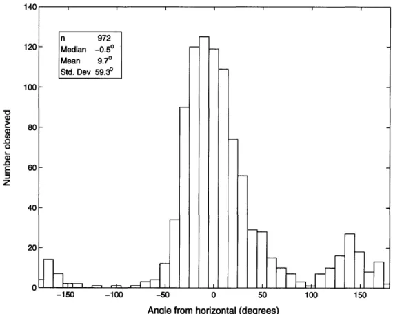
3.3.1 In situ observations of krill orientation ... ... 90
3.3.2 Scattering model predictions... 92
3.3.3 Model verification with empirical in situ target strength observations ... 95
3.4 D ISC U SSIO N ... ... 97
3.5 CONCLUSIONS... 106
ACKNOWLEDGMENTS ... 107
Chapter 4
-
Krill Distribution Along the Western Antarctic Peninsula and
Associations With Environmental Features, Assessed Using
Multi-Frequency Acoustic Techniques
4.1 INTRODUCTION ...
109
4.2 METHODS ...
114
4.2.1 Study area ...
114
4.2.2 Data collection ... 115
4.2.3 Acoustic analyses... 117
4.2.4 Estimation of krill biomass ... 125
4.2.5 Analysis of krill distribution in relation to environmental features ... 131
4.3 RESULTS ... 135
4.3.1 Application and verification of acoustic methodologies ... 135
4.3.2 Krill distribution... 154 4.4 DISCUSSION ... 182 4.4.1 Acoustic methodologies... 182 4.4.2 Krill distribution... 189 4.5 CO N CLU SIO N S... 199
ACKNOWLEDGMENTS ...
200
Chapter
5 -
Krill Aggregation Structure and Vertical Migration in Relation
to Features of the Physical and Biological Environment
5.1 INTRODUCTION ... 203
5.2 METHODS ... 206
5.2.1 Study area... 206
5.2.2 Data collection ... 207
5.2.3 Acoustic data analysis... 208
5.2.4 Measurements of aggregation features ... 212
5.2.5 Measurements of environmental properties ... 214
5.2.6 Statistical analyses ... 217
5.2.7 Analysis of individual aggregations ... 218
5.3 R E SU LT S ... 218
5.3.1 Diel patterns ... 224
5.3.2 Influence of krill length ... 232
5.3.3 Environmental influences ... 232
5.3.4 Influence of predators ... 243
5.3.5 Variability in density and size within individual aggregations... 258
5.4 DISCUSSION ... 263
5.4.1 Strengths and weaknesses of the acoustic analyses ... 265
5.4.2 Diel vertical migration ... 268
5.4.3 Variability in aggregation size ... 276
5.4.4 Behavior in relation to krill length... 277
5.4.5 Intra-aggregation variability in animal density and size ... 278
5.5 C O N CLU SIO N S... 280
Chapter 6 - Conclusions
6.1 ANTARCTIC ZOOPLANKTON ACOUSTICS ... ... 2836.2 ANTARCTIC KRILL ECOLOGY... 286
6.3 RELATION TO OTHER WORK... 289
6.4 BROADER IMPACT ... 294
Chapter 1
Introduction
1.1 MOTIVATION
The distribution of zooplankton is characterized by extreme variability at a range of spatial and temporal scales (Cassie, 1963; Haury et al., 1978); 'patchiness' is the term used to describe the intermittent nature and strong spatial heterogeneity typical of the distribution of many animals (Steele, 1974). Zooplankton patchiness likely stems from a complex interaction of physical processes, food availability, population dynamics, predation, and behavior (Folt and Bums, 1999). As a characteristic feature of marine systems, zooplankton patchiness must be taken into account in any consideration of ecosystem processes such as predator-prey interactions or carbon flux. In addition, patchiness has important consequences to the error associated with abundance estimates from low-resolution sampling techniques such as net surveys, and thereby to stock
assessment surveys for commercially-exploited species (McClatchie et al., 1994). Despite this convincing impetus, however, a comprehensive understanding concerning
zooplankton patchiness remains elusive, perhaps due to an historical lack of appropriate tools able to resolve small-scale variability (Greene et al., 1998).
Zooplankton play a pivotal role in the antarctic continental shelf ecosystem, providing both a trophodynamic link between phytoplankton and higher predators, and, via their faecal pellets, a mechanism by which newly fixed carbon can be exported from the euphotic zone (Priddle et al., 1992). The Southern Ocean is estimated to be responsible for 15% of global primary production (Huntley et al., 1991), much of which is consumed
by zooplankton. Understanding heterogeneity in the distribution of zooplankton as it relates to heterogeneity in that of primary producers is thus key to understanding carbon export in this important region, and to predicting the likely impacts of climate change.
Among antarctic zooplankton, much attention has focused on the Antarctic krill (Euphausia superba Dana), as the subject of one of the world's largest crustacean fisheries (Ichii, 2000), and the key prey item for numerous species of birds, seals, and whales (Laws, 1985). Many of these seal and whale species have still not recovered from over-exploitation in previous decades and centuries, such that understanding the
interaction of krill and their predators, and the potentially competitive impact of the krill fishery, is of great importance (Everson, 2000a). In addition, the krill is notable for its consistent formation of highly cohesive aggregations, and is a strong swimmer capable of overcoming most prevailing currents (Hamner et al., 1983). It therefore represents an attractive model species for the study of how active behaviors interact with physical oceanographic processes to generate patchiness in the distributions of zooplankton.
This thesis examines the forces that drive zooplankton distribution and patchiness in antarctic continental shelf regions, with particular attention given to the krill. The ultimate goal is to understand how physical oceanographic processes and environmental conditions are linked to krill distribution at the broad-scale and behavior at the level of the individual aggregation. The work is motivated both by the fascinating nature of the phenomenon of zooplankton patchiness in its own right, and by a desire to understand how krill distribution and behavior are linked to the dynamics of higher predators and the Southern Ocean ecosystem as a whole.
1.2 BACKGROUND
1.2.1 History of krill research and the krill fishery
Early recognition of the central importance of Antarctic krill to the diets of many higher-level Southern Ocean predators was made by the sealers and whalers of the 19th and 20th
centuries (summarized in Marr, 1962). Ecological interest in krill originated in attempts to manage the whale hunt on a scientific basis, resulting in the highly ambitious
Discovery Expeditions of the 1930s and 40s. The collected reports of the Expeditions painted the picture of an enormously abundant species, distributed in vast swarms about the entire antarctic continent (Marr, 1962), and which displayed a complex succession of life history stages (Fraser 1936). These somewhat qualitative studies laid the foundation for all later krill research.
With the precipitous decline in the whale catch during the 1960s (Laws, 1977), the potential of Antarctic krill as an apparently vast source of protein began to be considered (Moiseev, 1970). Estimates of krill abundance of the day ranged from 14 to 7000 million metric tons (Mt), implying the potential for a major fishery. Of particular notoriety was the 'krill surplus' hypothesis, which held that the deficit of 41.7 Mt of whale biomass culled by the whaling industry must have led to a 'surplus' annual production of 150 Mt of krill no longer being consumed and thus available for harvest (Gulland, 1970). Despite the concern of some that this potential surplus would simply be consumed by increasing populations of other apex predators (Laws, 1977), the notion of a harvestable 150 Mt at a time when the total combined yield of the world's fisheries was 60 Mt led to enormous optimism that a krill fishery would solve the problem of "supplying ever-increasing human populations with food" (Moiseev, 1970). Soviet exploratory fishing operations had demonstrated that krill were easy to find and catch (Makarov et al., 1970), and so by the end of the 1970s the krill fishery had begun in earnest. The Southern Ocean krill fishery peaked at a total catch of 0.5 Mt in the 1980s and presently extracts
approximately 0.1 Mt of krill annually, and thus is among the largest crustacean fisheries in the world (Ichii, 2000).
Recognition of the central role played by the krill in the antarctic marine ecosystem, coupled with the memory of the drastic over-exploitation of the Southern Ocean seal and whale populations of previous decades and centuries, however, has led to concerns that even light levels of fishing pressure might lead to a collapse of the food web (Nicol, 1994). Many antarctic top predators are dependent on krill as their primary prey item, and population dynamics for some species have been shown to vary with krill abundance, at least at a local scale (Reid and Croxall, 2001). This introduces the possibility of
competition between the commercial fishery and natural predators. The linkages between the dynamics and distribution of krill populations and those of their predators thus represent an important avenue of investigation.
Scientific interest in krill has also been prompted by the role this highly abundant secondary producer might play in global carbon cycling and its response to climate change. The extent to which the vast area of the Southern Ocean sequesters atmospheric carbon dioxide is of global biogeochemical relevance (Huntley et al., 1991). As a central member of the Antarctic food web, krill may exert a substantial influence over the degree to which carbon dioxide drawn down from the atmosphere and fixed into organic
particulate material by primary producers is exported from the shallow euphotic zone where primary production occurs and sequestered in the deep ocean (Priddle et al., 1992). The dense fecal pellets of krill and other zooplankton are known to constitute an
important mechanism for such carbon export (LeFevre et al., 1998), and the abundance and spatial distribution of the krill, in relation to that of primary producers, are likely to be important considerations in the Southern Ocean carbon cycle.
1.2.2 Ecology of the Antarctic krill
There are seven species of commonly occurring euphausiid in the Southern Ocean: Euphausia superba, E. crystallophorias, E. vallentini, E. triacantha, E. frigida, and
Thysanoessa macrura and T. vicina. The distributions of these various species show a great deal of overlap, but there is a general latitudinal gradation, with E. crystallorophias
mostly limited to continental shelf regions, E. vallentini restricted to waters north of the Antarctic polar front, and the other species found in between (Mauchline, 1980c;
Everson, 2000b). Of these species, perhaps the most abundant, and certainly the most commercially important, is the Antarctic krill, Euphausia superba.
The Antarctic krill has a circumpolar distribution strongly linked to large-scale
circulation features and characterized by enhanced concentrations located in two bands about the continent: one in continental shelf regions within the westerly-flowing East Wind Drift, and the other in oceanic waters between the easterly-flowing Antarctic Circumpolar Current (ACC) and the Antarctic Polar Front (Marr 1962; Amos, 1984). Both regions display large temporal variability in krill abundance between seasons (e.g., Lascara et al., 1999) and years (e.g., Brierley et al., 1997). The seasonal advance and retreat of the pack ice (from 20 million km2 in winter to 4 million km2 in summer) is generally believed to have a strong influence on the broad-scale distribution of krill, both through direct effects and indirectly through the association of the retreat of the ice with enhanced primary productivity at the ice edge (Miller and Hampton, 1989). Krill
distribution also varies meridionally, with particularly enhanced abundances found in the Ross, Weddell, and Bellingshausen Seas, along the western Antarctic Peninsula, in the western Scotia Sea around the productive krill fishing grounds of South Georgia, and in the region south of the Indian Ocean (Figure 1.1; Amos, 1984). Genetic analysis of krill mitochondrial DNA from some of these regions has suggested that krill near South Georgia are genetically distinct from those of the Weddell Sea, although otherwise no differences were found for krill sampled from these two location as well as the Ross and Bellingshausen Seas (Zane et al., 1998).
The krill is a long-lived species, reaching ages of 6-7 years, and spawning at age 2-3 during the summer in oceanic waters along or beyond the continental shelf break (Siegel, 2005). There is some suggestion that post-spawning adult krill then migrate in fall to over-winter in coastal regions (Siegel, 1988). Surveys in the Gerlache Strait along the Western Antarctic Peninsula have suggested that some krill, particularly small adults,
900 W
1800
900 E
Figure 1.1 - The antarctic continent, showing major seas and the location of the U.S. Southern Ocean GLOBal ECosystems Dynamics (SO GLOBEC) program study site.
may also spawn in the deep basins and troughs of more coastal regions (Brinton, 1991). The developing embryos sink and hatch at depths greater than 700 m (Siegel, 2000). Post-hatch larvae progress through a series of developmental stages as they migrate upwards to shallower waters by fall and are thought to spend the winter in association with the immediate under-ice environment (Marr 1962; Nicol, 2006). Some evidence suggests that krill recruitment is highest after winters of extensive sea-ice, and is influenced by competition with salps for phytoplankton food resources (Loeb et al.,
1997). Larval krill as small as 10 mm have been observed to form aggregations under sea ice (Hamner et al., 1989), and post-larval krill are thought to spend the majority of their time in aggregations. The high degree of cohesion and synchronized behavior in such aggregations revealed by the observations of divers has led some authors to suggest that the term 'school' is in fact most appropriate (Hamner et al., 1982), and the persistent occurrence of krill in aggregations has led others to suggest that the krill aggregation constitutes the basic ecological unit of the species (Watkins, 1986).
The emphasis of the present work is on the distribution of krill at the meso-scale and the structure and behavior of individual krill aggregations. More thorough reviews of the current state of understanding of these topics will be presented as introductory material in subsequent chapters. These subjects have received substantial attention, and interesting insights have emerged concerning the associations of krill with both physical
oceanographic and biological factors. Most of this previous work has been conducted during the austral spring and summer, however, when antarctic continental shelf regions are most accessible. Previous studies of krill distribution and aggregative behavior in fall and winter have been few, and it is in addressing this deficiency that this work makes one of its most important contributions.
1.2.3 Southern Ocean GLOBEC program
The present research was conducted as one component of the U.S. Southern Ocean GLOBal ECosystems Dynamics (SO GLOBEC) program, one of the many GLOBEC
projects around the world, which in broad terms are charged with understanding
variability in the populations of marine organisms in response to environmental change. The SO GLOBEC program's primary objective is "to understand the physical and biological factors that contribute to enhanced Antarctic krill growth, reproduction, recruitment, and survivorship throughout the year" (Hofmann et al., 2002). The program's goals also include an understanding of what factors contribute to the
availability of krill to higher predators, including whales, seals, and penguins, and in this respect the program is quite unusual. The concurrent collection of information on
physical processes, nutrient dynamics, primary producers, zooplankton, as well as higher predators, provides an important opportunity to understand biological-physical linkages at all levels of the ecosystem.
The SO GLOBEC program selected as its primary study site the continental shelf region in and around Marguerite Bay, west of the Antarctic Peninsula (Figure 1.1). This region is thought to sustain large abundances of Antarctic krill (Marr, 1962; Lascara et al.,
1999), and may act as a source for the down-stream krill populations that support the major krill fishery around South Georgia (Atkinson et al., 2001; Fach et al., 2002). The area is also home to large populations of predators dependent on krill as their central prey (Fraser and Trivelpiece, 1996; Costa and Crocker, 1996). Few previous studies of the region have considered the fall and winter seasons (Lascara et al., 1999), although the region is hypothesized to be an important krill over-wintering ground. Given the general dearth of previous wintertime studies of krill anywhere about the Antarctic, and in the Marguerite Bay region in particular, the SO GLOBEC program targeted austral fall and winter for periods of detailed study. The program approached its goals through a combination of broad-scale survey cruises with an ice-capable survey vessel conducted concurrent to process-oriented studies by a second vessel, coupled with more long-term deployments of satellite tags affixed to predators, weather stations, drifters, and moored instrument packages (reviewed in Hofmann et al., 2002, and see references therein to individual projects).
The Marguerite Bay region is characterized by a variety of physical features that may contribute to its support of such a productive ecosystem. The regional hydrography is reviewed in greater detail in the chapters that follow, but in brief, large gyres (100-400 km in horizontal extent along-shelf, 100-150 km across-shelf) have been observed over the western Antarctic Peninsula continental shelf, and the Antarctic Circumpolar Current (ACC) is typically positioned immediately beyond the shelf break (Smith et al., 1999). The continental shelf is overall quite deep, often exceeding depths of 400 m, and is intersected by a number of deep troughs. Warm and nutrient-rich rich waters present at depth beyond the shelf-break are pumped up onto the shelf by the action of the ACC at the points where these troughs intersect the shelf break (Klinck et al., 2004). These intruding waters are thought to be an important driver of primary production in the region and the dominance of large diatoms over other primary producers (Prizelin et al., 2004). The entire region is covered by sea ice in winter and is ice-free in summer (Stammerjohn and Smith, 1996). The complex interplay of these various forcings undoubtedly has important impacts on the distribution of krill and other zooplankton in the region.
1.2.4 Zooplankton acoustics
Stock assessment for management of the krill fishery, understanding the role of krill in the Southern Ocean carbon cycle, and quantification of the interactions of the krill with its predators, all require an ability to measure accurately the distribution of krill
abundance. Estimation of krill abundance, however, is made difficult by the extreme spatial patchiness typical of the species, its enormous potential range (the area of the Southern Ocean is 36 x 106 km2), and limited access to much of this range because of sea-ice (Everson, 2000b). Early estimates of krill abundance were derived from broad extrapolations of sparse measurements of krill density made with nets, or indirectly from calculations of the potential abundance of krill that could be supported based on
measured levels of primary production (e.g., Gulland, 1970). These estimates were generally high and showed little consistency between studies. A turning point was reached in the late 1970s, when the Biological Investigations of Marine Antarctic
Systems and Stocks (BIOMASS) research initiative focused attention on the use of hydroacoustics to quantify krill abundance (Everson and Miller, 1994).
High-frequency acoustic sensors are ideally suited to the study of zooplankton
distribution and patchiness, due to their fast sampling rates and concomitant ability to survey a large fraction of the water column at high resolution over large areas (Foote and Stanton, 2000). Acoustic techniques are particularly powerful when applied in
conjunction with independent measurements of the physical and biotic environment (e.g., hydrographic casts, net and video samples). In the Antarctic, acoustic sensors are now used routinely in ecological studies of krill, as well as in the stock assessment surveys employed in managing the krill fishery (see review by Hewitt and Demer, 2000).
Acoustic techniques rely on the fact that many marine organisms scatter sound in a predictable manner. Measurements of the intensity of echoes returned from sonic pulses emitted into the water column therefore can be used to make estimates of more
biologically-meaningful quantities such as animal abundance and size. This process of inferring the abundance and distribution of zooplankton in a quantitative sense from acoustic measurements, however, is not straightforward (Stanton et al., 1994; Wiebe et al., 1996). Scattering in the water column can result from both physical oceanic processes (e.g., microstructure; Warren et al., 2003) and the biota, where scattering from the latter is a complex function of the taxonomic composition of animals present, and the
associated variability in their size, shape, physical properties, and behavior. Accurate inference of organismal parameters such as abundance from acoustic measurements thus requires a comprehensive understanding of the scattering processes involved.
In the Antarctic, substantial progress has been made in discriminating Antarctic krill from other acoustic scatterers that may be present (reviewed in Watkins and Brierley, 2002). Historically, however, many Southern Ocean acoustic studies have simply assumed that all acoustic measurements above some minimum threshold level stemmed solely from krill (e.g., Macaulay et al., 1984; Lascara et al. 1999), thereby discarding potential
information on the abundance and distribution of other zooplankton, and possibly resulting in an overestimation of krill abundance. Discrepancies also exist in the predictions of the scattering by individual krill (i.e., target strength) from the semi-empirical model developed by Greene et al. (1991) that is in common use for krill surveys and theoretical models based on scattering physics (e.g., Stanton et al., 1993,
1998; McGehee et al., 1998). Target strength is a critical quantity in making abundance estimates from acoustic data, and the Greene et al. (1991) model marked a substantial improvement over earlier target strength models developed during the BIOMASS program (see review in Miller and Hampton, 1989), but these discrepancies have yet to be fully reconciled. Furthermore, developments made in zooplankton acoustics elsewhere involving the use of multi-frequency acoustic data to estimate simultaneously the
abundance and size of animals (e.g., Warren et al., 2003) have as yet not been applied in the Southern Ocean beyond individual test-case krill aggregations. Thus while the field of Antarctic krill acoustics has achieved a reasonable level of sophistication, there still exist opportunities for improvement.
It is important to note that even the advanced acoustic methodologies developed and employed in the present work are unable to distinguish at the specific level between the various species of aggregating euphausiids that may be present in the region (notably Euphausia superba and E. crystallophorias, and possibly Thysanoessa macrura); below these species therefore will be referred to collectively as 'krill.' The consequences of this inability are explored later in relation to the ecological conclusions made in each thesis chapter.
1.3 OBJECTIVES AND THESIS STRUCTURE
In this thesis, I examine the physical and biological forces that drive the distribution and patchiness of zooplankton in an antarctic continental shelf region. Both the broad-scale distribution of animals across the continental shelf and the scale of individual krill aggregations are considered. This is achieved by the application of a suite of sensors,
including multi-frequency acoustic, video, and net sampling systems, of which acoustic instruments provide the majority of the data considered. As such, an important
component of the research involves the development and verification of methods for extracting estimates of ecologically-meaningful quantities such as animal abundance
from measurements of scattered sound. The study area is that selected by the Southern Ocean GLOBEC program, the continental shelf region in and around Marguerite Bay, west of the Antarctic Peninsula, and the survey period the falls and winters of 2001 and 2002.
The thesis research is divided into four inter-related components, each of which has been prepared as a stand-alone document intended for publication as a refereed journal article, and each of which is presented here as a thesis chapter. Consequently, there is some redundancy in the various chapters, most notably in their respective introductions.
Chapters 2 and 3 repeat mostly verbatim the material of Lawson et al. (2004) and Lawson et al. (2006), respectively; the changes made here to the text of those publications were done in an effort to keep the language consistent with the rest of the thesis.
Chapter 2 takes an overview-approach to the question of the distribution of zooplankton and micronekton in the study region. Spatial and temporal patterns in the distribution of acoustic volume backscattering strength at a single frequency during the fall and winter of 2001 are examined, as a coarse index of the overall biomass of zooplankton and micronekton. These patterns are considered in light of hydrographic features of the region. Calculations are then made of the likely taxonomic composition of animals responsible for the observed levels of volume backscattering, based on net catches and models of how individual animals scatter sound. This exercise demonstrates that euphausiids were the dominant scatterer at only very particular locations and depths, emphasizing the need for caution when seeking to study euphausiids separately from other zooplankton using acoustic data.
Motivated by discrepancies that emerged during the analyses of Chapter 2 between theoretical and empirical approaches to understanding acoustic scattering by Antarctic krill, Chapter 3 seeks to improve parameterization of a theoretical scattering model on the basis of direct measurement of all necessary model parameters for animals sampled in the study region and survey period. This novel parameterization is then verified on the basis of comparisons of model predictions to in situ observations of krill target strength (i.e., the level of scattering from one animal). This chapter thus establishes a validated krill target strength model for the acoustic analyses of krill distribution that follow in later thesis chapters.
Chapter 4 builds on the analyses of Chapter 2 by focusing in particular on the distribution of krill in the study region, and expanding to a consideration of both survey years. Given its broad-scale survey coverage and high resolution, this is again done on the basis of the acoustic dataset, although unlike Chapter 2, the full multi-frequency dataset is employed. The first component of the chapter involves the development of methods that capitalize on differences predicted by the model of Chapter 3 between the scattering of krill versus that of other taxa and in the scattering of krill of different sizes, in order to identify krill aggregations in the acoustic data, and then estimate the length, abundance, and biomass of constituent members. These methods are verified through comparisons to independent net and video samples. In the second component of the chapter, these methods are applied to the full multi-frequency dataset collected during all four broad-scale surveys of the study region. The resultant descriptions of the temporal (seasonal and inter-annual) and spatial (vertical and horizontal) variability in distribution of krill along-track biomass are then considered in relation to aspects of the physical and biological environment.
Chapter 5 complements the examination of the distribution of krill aggregation biomass conducted in Chapter 4 by focusing on the characteristics of individual acoustically-identified krill aggregations, in order to make inferences concerning the behaviors and forces underling krill aggregation and diel vertical migration. The morphology, internal structure, and vertical position of aggregations are considered in relation to a variety of
properties of the physical and biological environment, including time of day, food availability, currents, and the occurrence of predators. In addition, aggregation characteristics are studied relative to the acoustically-estimated mean length of constituent members in order to identify size- or age-related changes in aggregative behavior. Certain large aggregations are also selected for more detailed examination of
intra-aggregation variability in krill length and density.
Chapter 6 then provides a summary of the major findings of the research and their broader significance. In particular, the implications of the present work to the field of zooplankton acoustics and to current understanding of the interactions between krill and higher predators, including whales, seals, and birds, are considered.
Chapter
2
Acoustically-Inferred Zooplankton
Distribution in Relation to Hydrography
West
of the Antarctic Peninsula
ABSTRACT
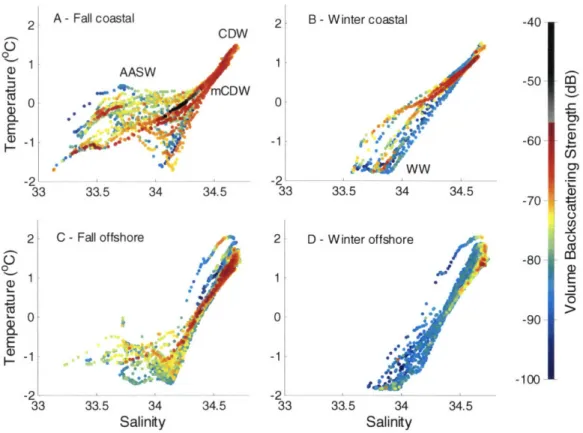
The relationship between the distribution of zooplankton, especially euphausiids (Euphausia and Thysanoessa spp.), and hydrographic regimes of the Western Antarctic Peninsula continental shelf in and around Marguerite Bay was studied as part of the Southern Ocean GLOBEC program. Surveys were conducted from the RVIB N.B. Palmer in austral fall (April-June) and winter (July-August) of 2001. Acoustic, video, and environmental data were collected along 13 transect lines running across the shelf and perpendicular to the Western Antarctic Peninsula coastline, between 65 and 70'S. Depth-stratified net tows conducted at selected locations provided ground-truthing for acoustic observations. In fall, acoustic volume backscattering strength at 120 kHz was greatest in the southern reaches of the survey area and inside Marguerite Bay, suggestive of high zooplankton and micronekton biomass in these regions. Vertically, highest volume backscattering was in the depth range from 150 to 450 m, associated with modified Circumpolar Deep Water (CDW). The two deep troughs that intersect the shelf break were characterized by reduced volume backscattering, similar to levels observed off-shelf and indicative of lower zooplankton biomass in recent intrusions of CDW onto the continental shelf. Estimates of dynamic height suggested that geostrophic circulation likely caused both along- and across-shelf transport of zooplankton. By winter, scattering
had decreased by an order of magnitude (10 dB) in the upper 300 m of the water column in most areas, and high volume backscattering was found primarily in a deep (> 300 m) scattering layer present close to the bottom. The seasonal decrease is potentially
explained by advection of zooplankton, vertical and horizontal movements, and
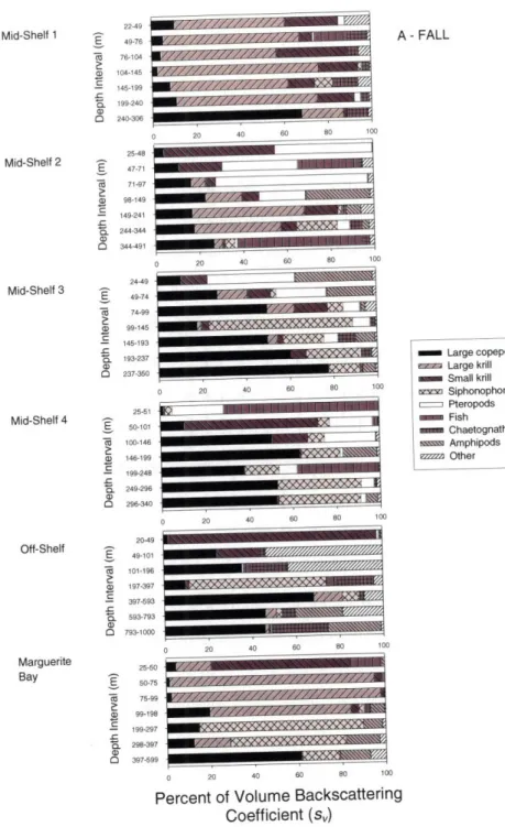
mortality. Predictions of expected volume backscattering strength based on net samples suggested that large euphausiids were the dominant scatterer only at very particular locations and depths, and that copepods, siphonophores, and pteropods were more important in many locations.
2.1 INTRODUCTION
Zooplankton play a pivotal role in the antarctic continental shelf ecosystem, providing both a trophodynamic link between phytoplankton and higher predators, and, via their fecal pellets, a mechanism by which newly fixed carbon can be exported from the
euphotic zone (Priddle et al., 1992). Historically, much attention has focused on Antarctic krill (Euphausia superba) due to its status as a key prey item for many whales, birds, seals, and fishes (Laws, 1985) and as the subject of a commercial fishery (Ichii, 2000). Although less studied, other zooplankton also represent important ecosystem members: copepods, for example, frequently exceed Antarctic krill in abundance and are the main prey of invertebrates, sei whales, and fish (Voronina, 1998), while salps may account for more carbon export to depth than Antarctic krill (Le FRvre et al., 1998).
High-frequency acoustic sensors are often used in the study of zooplankton distribution, due to their high sampling rates and concomitant ability to survey the entire water column over large areas (Foote and Stanton, 2000). In the Antarctic, acoustic techniques are used
routinely to survey the biomass and distribution of Antarctic krill (see review by Hewitt and Demer, 2000), but have been used much less frequently to study other zooplankton taxa (Weeks et al. 1995; Brierley et al., 1998). Substantial progress has been made in discriminating Antarctic krill from other acoustic scatterers that may be present
2003). Historically, however, many Southern Ocean acoustic studies have simply assumed that all volume backscattering strength measurements above some minimum threshold stemmed from Antarctic krill (e.g., Macaulay et al., 1984; Lascara et al. 1999; Nicol et al., 2000). The contribution to acoustic observations from other zooplankton taxa often has been assumed to be negligible, which discards potential information on the biomass and distribution of such taxa, and may result in an overestimation of Antarctic krill abundance.
The continental shelf region in and around Marguerite Bay, west of the Antarctic Peninsula (Figure 2.1), is hypothesized to be an important over-wintering ground for Antarctic krill, and may act as a source for the down-stream krill populations in the Bransfield Strait and at South Georgia (Atkinson et al., 2001; Fach et al., 2002). Little is known about the distribution of Antarctic krill or other zooplankton in this area during winter, however, although studies of the nearby Bransfield Strait region have been more numerous (e.g., Siegel 1989; Zhou et al., 1994). In the only previous acoustic survey of the region, Lascara et al. (1999) examined Antarctic krill distribution in Marguerite Bay and the region immediately to the north, and found distinct seasonal variability in biomass and vertical distribution, with krill more abundant and found shallower during
the summer and spring than fall and winter. The acoustic system employed reached to only 189 m in depth, and so this study was unable to conclude whether the seasonal decrease in biomass resulted from vertical or horizontal movements. Given the dearth of previous studies, the U.S. Southern Ocean GLOBal ECosystems Dynamics (SO
GLOBEC) program has targeted austral fall and winter as periods for detailed study of the Marguerite Bay region (Hofmann et al., 2002). The program's primary objective is to understand the physical and biological factors that contribute to Antarctic krill over-wintering success. As such, one goal of the program is to link physical processes with the distribution of Antarctic krill and other members of the zooplankton community, and ultimately with higher predators.
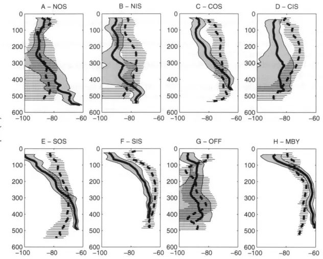
B - SURVEY BLOCKS
C -FALL D -WINTER
78 W 75 W 72 W 69 W 66 W
Figure 2.1 - U.S. SO GLOBEC survey area. Shown are (A) the overall geographical context of the survey area, (B) the location of survey blocks, and the cruise tracks in (C) fall and (D) winter of 2001. The latter show only those portions of the overall cruise-track where acoustic data were collected. Note the lower survey coverage in winter relative to fall. Block name abbreviations are: Northern Outer-Shelf (NOS), Northern Inner-Shelf (NIS), Central Outer-Shelf (COS), Central Inner-Shelf (CIS), Southern Outer-Shelf (SOS), Southern Inner-Shelf (SIS), Off-Shelf (OFF), and Marguerite Bay (MBY). Circles indicate where the MOCNESS tows analyzed here were conducted, with tow locations abbreviated as mid-shelf 1-4 (MS 1-4), off-shelf (OS), and Marguerite Bay (MBY). Gray arrows show where the deep troughs that run diagonally across the continental shelf meet the shelf break.
66 67 68 69 70 A- STUDY AREA
In this paper, we describe measurements of acoustic volume backscattering strength made over most or all of the water column during austral fall and winter of 2001, in relation to hydrography in the vicinity of Marguerite Bay. We then use depth-stratified net samples and taxon-specific models of acoustic target strength to predict the likely sources of scattering, with particular emphasis on understanding the contribution of zooplankton taxa other than Antarctic krill. On the basis of these measurements and predictions, we make certain inferences concerning seasonal and spatial variability in zooplankton and micronekton biomass in the region.
2.2 METHODS
2.2.1 Study area
The U.S. SO GLOBEC Program study site was located on the continental shelf to the west of the Western Antarctic Peninsula, extending from the northern tip of Adelaide Island to the southern portion of Alexander Island and including Marguerite Bay (Figure 2.1). Two cruises were conducted in the area on the RVIB Nathaniel B. Palmer: a cruise during austral fall from April 23 to June 6, 2001 (cruise number NBP0103), and a cruise during winter from July 21 to September 6, 2001 (cruise number NBP0104). The cruise track in fall was determined by the position of 84 station locations distributed along 13 transect lines spaced 40 km apart and running across the continental shelf and
perpendicular to the Peninsula coastline. On the winter cruise, eight additional stations were added to the survey grid and the entire grid was shifted south by two kilometers so that acoustic mapping of the sea floor would take place over unmapped sea floor. In order to allow spatial comparisons across the region, the overall study area was subdivided into eight functional blocks (Figure 2.1b). The survey region first was subdivided from
northeast to southwest into three sectors (southern, central, and northern), each of which was divided into inner-shelf (i.e., coastal) and outer-shelf blocks. An off-shelf block was defined as the region beyond the 1000 m isobath, and a final block corresponded to the interior of Marguerite Bay.
2.2.2 BIOMAPER-II
The BIo-Optical Multi-frequency Acoustical and Physical Environmental Recorder, or BIOMAPER-II, is a towed system designed to conduct quantitative surveys of the spatial
distribution of plankton and nekton (Wiebe et al., 2002). The system consists of a multi-frequency echosounder, a Video Plankton Recorder (VPR, Davis et al., 1992), and an environmental sensor package (Conductivity, Temperature, and Depth sensor (CTD); fluorometer; transmissometer). To enhance the performance of the BIOMAPER-II in high sea states, a slack tensioner was used to damp the motion of the ship (see Wiebe et al., 2002 for additional details).
2.2.2.a Acoustic definitions
Volume scattering strength, or S, (where Sv = 10loglo(sv) in units of decibels relative to 1 m-', and s, is the observed volume scattering coefficient), is a measure of the intensity of emitted sound that is scattered towards the acoustic receiver per cubic meter. When the
source and receiver are co-located, the direction of scattering is back towards the source, and this quantity is commonly referred to as the volume backscattering strength. Under the assumption made in zooplankton acoustics that scattering from individual targets in the ensonified volume sums incoherently, the volume backscattering strength is equal to the sum of the scattering contributions from each target, normalized by the sample volume. For simplicity, this quantity of measured backscattered sound per unit volume will be referred to as 'volume backscattering' and we will distinguish between the arithmetic and logarithmic forms of 'volume backscattering coefficient' and 'volume backscattering strength' only when necessary.
Volume backscattering is related to both the number and size of scatterers in the path of the incident sound, to the efficiency with which these objects scatter sound, and thereby to their taxonomic composition. Although the relationship between volume
large spatial and temporal differences in volume backscattering observed in the present study are related to differences in zooplankton and micronekton biomass. In the
discussion we show how the confounding influences of animal size, sound scattering efficiency, and taxonomic composition, are minimized in this study.
2.2.2.b Acoustic data collection
The BIOMAPER-II collected acoustic data from five pairs of transducers, with frequencies of 43, 120, 200, 420, and 1000 kHz. All transducers had 3 ' half-power beamwidths, with the exception of the 43 kHz transducers, which had beamwidths of 7 . One of each pair of transducers was mounted on the top of the tow-body looking upward, while the other was mounted on the bottom looking downward. This arrangement
allowed acoustic data to be collected over most or all of the water column as the instrument was 'towyoed' obliquely up and down through the water column between depths of 20 and 300 m. The vessel proceeded along the track-line between stations at speeds of 4 to 6 knots, and surveying was conducted around the clock.
Multi-frequency acoustic data were collected over much of both surveys, although prohibitively thick pack ice in portions of the survey area led to the area surveyed in winter being less than in fall (Figure 2. lc,d). Due to episodic malfunctions at the different acoustic frequencies, 120 kHz represents the frequency at which data were collected with the greatest spatial coverage. In order to allow examinations of the seasonal distribution of zooplankton over the broadest scales possible and best complement the scales at which data were collected by other projects conducted during the cruises (e.g., top predator surveys), this paper deals only with acoustic data collected at 120 kHz. Analyses of the multi-frequency data will be the subject of future work.
Measurements of volume backscattering at 120 kHz were collected in intervals of 1.5 m in vertical extent, starting at 6 m from the transducer face (the end of the acoustic near-field) and extending to a maximum range of 300 m from the instrument. A 10 kHz
bandwidth chirp pulse was used (Ehrenberg and Torkelson, 2000), with an effective pulse duration of 0.18 ms, and a ping rate of 0.3 pings s-'. The system's dynamic range allowed these data to be collected between -100 and -40 dB. Profiles of noise levels (ship's noise, ambient noise, and system noise combined) vs. depth were made in situ near the start of each cruise. Volume backscattering measurements for each ping were compared to these profiles, and those bins where measured volume backscattering did not exceed noise levels were set to zero. Each measurement was the result of echo-integration performed over a 4-ping interval (i.e., -35 m along-track).
All transducers were calibrated by the manufacturer (Hydroacoustic Technologies Inc., Seattle, WA, USA) prior to each cruise for source level, receive sensitivity, as well as transmit and receive beam patterns. An in situ calibration also was performed at the end of the winter cruise with a 38 mm tungsten carbide (6% cobalt) standard target, following established practices (Foote et al., 1987). After volume backscattering data were
normalized by the results of these calibrations, there was evidence of higher volume backscattering levels observed by the up-looking 120 kHz transducer relative to the down-looking transducer in some portions of the water column (Figure 2.2). This
discrepancy was particularly evident in low-scattering areas such as the northern portion of the survey area in fall, and much of the continental shelf during winter; in
high-scattering areas like Marguerite Bay, no such difference was evident. Furthermore, the enhanced volume backscattering in the up-looking data was restricted to the pycnocline and was especially prominent in regions of rapid vertical changes in density. We believe that these enhancements do not represent scattering from biological sources, but rather represent an as-yet unexplained artifact. They may result from sound scattering off vortices shed by the tow cable as it passes through the pycnocline. Since the tow cable extends above the towed body, only the up-looking transducer would observe such artifactual scattering. It therefore was excluded from all quantitative analyses, representing a 7% reduction in data (varying from 0 to 24% on a by-transect basis), primarily between depths of 0 and 200 m.
-65.
-67
-78 "
-100 -90 -80 -70 -60 -50 -40
Volume Backscattering Strength (dB)
Figure 2.2 - Acoustic data collected in (A) fall and (B) winter of 2001. Volume backscattering strength is plotted on the color scale in decibels, according to the depth
and position of measurement. Blue indicates low levels of zooplankton volume
backscattering, while red to black indicate high levels. High volume backscattering near the surface corresponds to the surface bubble layer. Strong (i.e., black) returns at depth are from the strongly scattering bottom. Both the bottom and surface layer were edited out for quantitative analyses. The V-shape of the maximum depth of observation is due to the BIOMAPER-II being towyoed up and down through the water column as the vessel proceeded along-track. Arrows indicate typical regions of the pycnocline where enhanced volume backscattering measured by the up-looking transducer (i.e., in the upper portion of the towyo's V) was believed to represent an artifact rather than scattering from biological sources.
-65s INTER
-67
78 -77 ' w
Figure 2.2 -continued
2.2.2.c Acoustic data post-processing
Acoustic data from the up- and down-looking transducers were combined to provide a vertically-continuous acoustic record extending from the surface to a depth of at least 300 m, and at most 550 m, depending on the position of the BIOMAPER-II along its towyo path. This acoustic record then was edited using custom MATLAB-based routines to remove unwanted returns from the surface bubble layer and the bottom, as well as noise spikes from the ship's engines or ice-breaking.
For many of the following spatial analyses, measurements of volume backscattering in each 1.5-m depth bin were averaged over 1-km along-track intervals and also over depth, in intervals of 25 to 100 m (shallow layer), 100 to 300 m (mid-water layer), and 300 to 500 m (deep layer). These depth ranges were chosen since the surface bubble layer obscured most measurements shallower than a depth of 25 m, the mixed layer depth was generally around 100 m, and 300 m represents the depth to which the BIOMAPER-II always made acoustic observations despite being towyoed up and down through the water column. These averages, as well as all other simple descriptive statistics, were performed on the arithmetic quantity of the volume backscattering coefficient (s,). The arithmetic form also was used in between-block statistical comparisons, since the tests employed were rank-based (see below) and so insensitive to whether the data were transformed or not. The logarithmic quantity of the volume backscattering strength (S,) was used in regression analyses, since this test is parametric and the log-transformed data better approximated a normal distribution. The decibel form is also used in figures and in the text.
2.2.3 Environmental analyses
Acoustic data were combined with environmental data to examine the association of volume backscattering with environmental properties and water masses. Depth,
BIOMAPER-II along its towyo path at 4-second intervals. In order to provide details of the environmental structure at greater depths than sampled by the towed body, however, data from CTD casts made at the survey stations by Klinck et al. (2004) were used as the primary source for quantitative analyses. The CTD rosette package made measurements of salinity, fluorescence, transmittance, photosynthetically active radiation (PAR), potential temperature, and oxygen concentration at 1-m depth intervals from the surface to between 5 and 20 m off the bottom. In analyses of volume backscattering in relation to environmental conditions, each environmental measurement was associated with the acoustic measurement averaged in 1-km intervals made nearest to that depth and location.
2.2.4 MOCNESS
A 1-m2 Multiple Opening/Closing Net and Environmental Sensing System (MOCNESS; Wiebe et al., 1985) was used to sample the zooplankton at selected stations distributed throughout the survey grid (24 locations in fall and 17 in winter). The MOCNESS was equipped with nine 335 gLm mesh nets, a suite of environmental sensors including
temperature, conductivity, fluorescence, and light transmission, and a strong strobe light, that flashed at 4-second intervals. The rationale behind the strobe system was to shock or blind the animals temporarily so that the net would not be perceived and avoided, and catches of large euphausiids were significantly enhanced when using the strobe (Sameoto et al., 1993; Wiebe et al., 2004). The MOCNESS was towed obliquely from near-bottom to the surface, sampling eight depth intervals on the up-cast. The deepest tows sampled to a depth of 1000 m. Typically, the upper 100 m was sampled in 25-m intervals, with 50-m intervals at intermediate depth ranges, and greater intervals (150- or 200-m) for the deepest depth ranges (see Ashjian et al., 2004, for additional details). The depth-specific
samples were preserved upon recovery in 4% buffered formalin.
The size distributions of plankton for six MOCNESS tows from each of the two cruises have been analyzed to date (Ashjian et al., 2004). Following the nomenclature of Ashjian et al. (2004), tow locations will be referred to as off-shelf, Marguerite Bay, and mid-shelf
1 -4 (Figure 2. l1c,d). Note that no acoustic data were collected in the vicinity of the mid-shelf 4 site during winter. Lengths of individuals of each sampled taxon were determined for an aliquot of each net sample using the silhouette method of Davis and Wiebe (1985).
2.2.5 Taxonomic composition of zooplankton and micronekton
The ultimate goal of our research is to use VPR observations and taxon-specific
differences in scattering at increasing frequencies, in addition to net catches, to partition accurately our measurements of volume backscattering among taxonomic groups, and then to make biomass estimates for each taxon. Here, we make preliminary inferences concerning the sources of acoustic volume backscattering measurements by conducting the forward problem: an exercise where predictions are made of expected volume backscattering strength based on MOCNESS catches and models of the scattering from
individual sampled animals (Wiebe et al., 1996). By comparing these predictions to observed levels, it is possible to assess whether the animals collected by the nets could
account for measured volume backscattering. Provided that this assessment is favorable, inferences can then be made about the likely relative contributions of different taxa to observed volume backscattering in the vicinity of each tow.
In addressing the forward problem, predicted volume backscattering for each depth stratum sampled by the MOCNESS was calculated as the linear (i.e., incoherent) sum of expected echo intensities from each captured animal. Expected echo intensities, or backscattering cross-sections (abs), were estimated based on the length of each individual
determined by silhouette analysis and models of acoustic scattering appropriate to the individual's taxonomic group. These models were developed by Stanton et al. (1994, 1998), are reviewed in Stanton and Chu (2000), and are sensitive to numerous parameters in addition to animal length, including animal orientation and material properties (Chu et al., 2000a; Table 2.1). Discrete values were used for all parameters other than animal orientation (Table 2.1). For the latter, scattering from each animal was averaged over
S0 u cd Es > tD _ )t 0 .0 C:L, to. 0 c 00 U 0 ~0 0 S-E ac~
a
~ ~c
ConEEs
00X 0 0 0) (:1 00
a cnc 00 0. cl 0 r S t 0~- > 3~ 0) s- 0 0 d 0s -~ l 0 *5 e d .f '; 0) 0 -o -6) 00* 9~ 00~e .0 _a .0 0 0 o ' " 30 0 ~i 'r < X:d
: ~ 0, S~,0 E 0~a ' o -5 a> S . 06 0~ ) 0) ~fZ *S~ -~ 4; 9 0 .0.006 o.0 0) ci ) 0 b 0 5 t .5 .5o " - 0..0 0) (n* 0F'~S~5c 5 - a ' 0~; o ea~ "EQ~ ~~ 0 Z 2 0 '= E~ ~ 0~ ~00;- 0E~u
-o -x Q-0).-cncE
ao
cn
006) C u a-a 0r 0Icn~
XUO0V0E~C~
0 -vj bb c t 9 '60 0 0 0 toL E) 00)0.0 -O 0) .L -a,~ CC~ 0 c bIoc0 S E~ Q) 0) C 0 00 0 .h 0$- Q ~ci~ 0 D 2 ~~ 0 0 ~4- ; 0) O.- 0 ·i~ E o55>~c 0.a 00)C m~ O.0 0)0 . $-0) - .0~ S -· c-n 0 0) 0 6 ~Y 0t) ca - 00 ,ja 0) 0O ,., 0 n .- 00) h c~,,· - 0 0: 0 0 0.'' oe s 00) Clct 0^ 0d 0O ON 0dr aO~ C,, $-a r 0 .z3 XQ 00.0.0C 0 00 ~ -0 0 o*~ = 000,,,f ;- r=.0 a O 0 d 0 ;- 0:~ 0 00 E-0 C ,, L ba.0 30)' I-Et .00; O~ 01 0-0 e 0.,-; 0014 0 N l 0)C o 0 0 0 = "• ¢0 0) 0 0) 0 .,,,0c M 0 ~o 0\ 00 a 0)u e
0. .0 0 -o 0 0 0) > .0 -' 0 O. 0 0, 0 0) 0. vl 0J 0) E .0u 00 -0j 0 Cl 0 O -o [" 0 0) Cl 00 a -O~p 0d "-;a 0.0 o 0)0 " 0)X~j5 - Cl cc C, 0) 0 0 CI-u 0) 0) 00 0 C C Ct C, > CA U 0 0 0b 0 0 0 0) Cf 0) $j~ P)C, -00 0~ 2 ba .00 ~ 0CI C,, V50 0 - n r-00 0 0 o 0Q 9z
z
~zz zz
z z
0) Z Z Z Z -o 0 5 U V $= )c u0 C~l 0) 1m rj.) ok 0L M * ctt cn 0 0 - 0) cn 5 o -e + E ooc E 00 II 00 0 0 0 0 0 -cl ~0 0 0 IC u 0) ,2 -o C~ = u oE r• cUsome distribution of orientations, to allow for the fact that the animals are oriented at a range of angles as they move through the water.
The calculations of the net-based forward problem involved summing estimates of expected backscattering cross-sections for each jth individual over all individuals in each
ith taxon and then over all taxa to yield an estimate of the total expected volume
backscattering strength in the volume (V) sampled by each kth net:
Svk =
10loglo
I1
(crbs
(2.1)
Since the BIOMAPER-II and the MOCNESS could not be towed concurrently,
comparisons of predicted volume backscattering strength could not be made to observed levels made at the identical time and location. Comparisons were thus made to acoustic observations made in the same depth interval and averaged over a spatial area within no more than 17 km of each of the 11 MOCNESS tows. At all but two MOCNESS tow locations, acoustic data were collected within no more than five hours of the net tow as the vessel approached or departed the station. At the mid-shelf 1 and 2 stations in winter, however, MOCNESS tows and acoustic data collection were separated in time by
approximately four weeks due to problems with the instruments malfunctioning.
Predictions of volume backscattering from each taxon were still calculated based on these tows, in order to shed light on the sensitivity of the predicted to observed volume
backscattering comparison to temporal variation.
2.3 RESULTS
Volume backscattering during fall generally was enhanced within Marguerite Bay and in the southern portion of the survey area (Figure 2.2a). Large sub-surface patches of