HAL Id: hal-00302947
https://hal.archives-ouvertes.fr/hal-00302947
Submitted on 7 Jan 2008
HAL is a multi-disciplinary open access
archive for the deposit and dissemination of
sci-entific research documents, whether they are
pub-lished or not. The documents may come from
teaching and research institutions in France or
abroad, or from public or private research centers.
L’archive ouverte pluridisciplinaire HAL, est
destinée au dépôt et à la diffusion de documents
scientifiques de niveau recherche, publiés ou non,
émanant des établissements d’enseignement et de
recherche français ou étrangers, des laboratoires
publics ou privés.
A model for aperiodicity in earthquakes
B. Erickson, B. Birnir, D. Lavallée
To cite this version:
B. Erickson, B. Birnir, D. Lavallée. A model for aperiodicity in earthquakes. Nonlinear Processes in
Geophysics, European Geosciences Union (EGU), 2008, 15 (1), pp.1-12. �hal-00302947�
www.nonlin-processes-geophys.net/15/1/2008/ © Author(s) 2008. This work is licensed under a Creative Commons License.
Nonlinear Processes
in Geophysics
A model for aperiodicity in earthquakes
B. Erickson1, B. Birnir1, and D. Lavall´ee2
1Department of Mathematics, University of California, Santa Barbara 2Institute of Crustal Studies, University of California, Santa Barbara, USA
Received: 20 August 2007 – Revised: 23 November 2007 – Accepted: 28 November 2007 – Published: 7 January 2008
Abstract. Conditions under which a single oscillator model coupled with Dieterich-Ruina’s rate and state dependent fric-tion exhibits chaotic dynamics is studied. Properties of spring-block models are discussed. The parameter values of the system are explored and the corresponding numerical so-lutions presented. Bifurcation analysis is performed to de-termine the bifurcations and stability of stationary solutions and we find that the system undergoes a Hopf bifurcation to a periodic orbit. This periodic orbit then undergoes a pe-riod doubling cascade into a strange attractor, recognized as broadband noise in the power spectrum. The implications for earthquakes are discussed.
1 Introduction
In the late 1960s, Burridge and Knopoff (BK) introduced a model that exhibited some characteristics similar to the dy-namics of an earthquake fault (Burridge and Knopoff, 1967). They were interested in the role that friction plays in regard to the earthquake mechanism and how successive events re-late to each other in time and space. The basic configuration of the BK model consists of a block coupled by a spring to a moving loader plate representing the other side of the fault (see Fig. 1). The equations of motion for this model include a friction term accounting for the roughness of the surface upon which the block slips. This term is a linear function of the velocity of the loader plate added to a viscous term pro-portional to the velocity of the block. Burridge and Knopoff wanted to see how many features observed in nature would be reproduced by their model.
Since its introduction, different variations of spring-block models have been shown to possess a power law distribution of event sizes similar to the Gutenberg-Richter law (Carl-son et al., 1994; Turcotte and Malamud , 2002; Bak et al., Correspondence to: B. Erickson
1987; Bak et al., 1988). Numerous studies and various im-provements to this model have been attempted (Pelletier, 2000; Gross, 2000; Clancy and Corcoran, 2005) in order to gain more realistic dynamics for simulations done to com-pare with laboratory experiments. Over the years it has been agreed upon that friction constitutive laws are one of the most important factors in improving the laboratory model, enabling them to exhibit effects more like those observed in an actual fault. Additional references and discussion of this can be found in the paper by Marone (1998).
In the early 80s, rate and state dependent frictions laws have shown to be qualified in reproducing some behavior similar to that of earthquake faulting. Burridge and Knopoff incorporated a friction term in their model that was depen-dent on the block’s velocity, but studies were later made that indicated that the friction term could not be a single valued function of velocity (Marone, 1998). Improvements to the BK friction law were made by Dieterich, Ruina, Rice and others based on empirical studies of rock friction in the lab-oratory. They discovered that the incorporation of a state variable enabled the model to exhibit almost entirely the ob-served seismic behaviors such as stick-slip phenomena, fault healing and memory effects (Ruina, 1983), (Marone, 1998). Carlson and Batista (1996) developed further constitutive re-lations to describe the friction in a lubricated interface, with the state variable representing the degree of melting in the lubricant layer. Daub and Cralon (2007)1have studied fault-scale behavior of various friction laws (including Dieterich-Ruina style friction) and their implications for dynamic rup-ture.
Dieterich-Ruina style friction in the spring-block model involves a logarithmic term whose nonlinearity has intro-duced additional difficulty in solving the problem. Due to the nonlinear term, analytic integration cannot be done even in the simplest case when one block is used. And while
1Daub, E. G. and Carlon, J. M.: A constitutive model for fault
gouge deformation in dynamic rupture simulations, J. Geophys. Res., submitted, 2007.
2 B. Erickson et al.: Aperiodic earthquakes
Fig. 1. The single degree of freedom block and spring model is a
slider coupled by a spring to a loader plate representing the other side of the fault. The surface upon which the block slips is rough and the friction force holding the slider in place is quite complex. Dieterich – Ruina style laboratory derived friction laws are used in this simulation for their capability in reproducing many qualitative dynamics similar to earthquake faulting.
numerical solutions can be computed, the logarithmic term still proves to be a challenge. Under laboratory determined values for the parameters, the system is extremely stiff in the numerical sense. Due to the nonlinear term, the main source of numerical stiffness, extremely small time steps must be taken even with implicit methods. In the past, the Dieterich-Ruina friction term has been altered because of this problem. In Lapusta and Rice (2003) and Szkutnik et al. (2003), the authors regularize the nonlinear friction term for values near zero. This can be done by either allowing rate values to be of either sign and taking absolute values or by linearizing the term giving only a close approximation in a small interval. Either this alteration of the nonlinear term or the lack of bet-ter solution algorithms (in Rice and Tse, 1986, for example) may explain why chaotic regimes have rarely been observed in simulations done with this friction law and realistic param-eter values.
In this paper we use the full nonlinear term in the numer-ics and find many different types of solutions to the system of a single block. Figure 2 shows the dynamics of the single block from Fig. 1, under such a new friction law, exhibiting periodic behavior. As shown later, this periodic orbit under-goes a period-doubling cascade into a strange attractor due to variations in the system’s parameters. Shkoller and Min-ster (1997) performed simulations and used unimodal maps to show that chaotic behavior was suggested by this friction force, although their parameter values do not seem to be re-alistic for earthquakes. In 1999, Drummond found dynamic regimes similar to ours while experimenting with lubricant
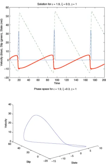
Fig. 2. Periodic solution to the Single-Degree of Freedom system
(2) with parameters ǫ=1.9, ξ =0.3, γ =1. Top: The slip value (green), characterizes the block sticking and slipping. The velocity (blue) is initially at zero, while the block is stuck. The slider remains stuck until the friction force holding it in place is overcome by the loading force. The velocity then spikes when the block slips and the slip value jumps almost instantaneously. The velocity then returns to zero, as the block becomes stuck and another cycle begins. θ (red) can be interpreted as the amount of asperity contact that the block has with the surface. While the block is stuck, the contacts steadily increase, until the block slips and the contacts instantly decrease. Bottom: periodic orbit in the corresponding phase space. Notice that the phase space is three-dimensional.
films subjected to shear. The measured friction force re-mained constant for the steady sliding phase, oscillatory be-tween two values for periodic phases, and even chaotic in a certain velocity range. These empirical results suggest that the nonlinearity of the friction force in these models is cru-cial for chaotic dynamics to emerge.
We integrate the dynamical system numerically, choosing parameter values that are commonly used in more recent
literature. Under the assumption that the friction law is the main physical process regulating the frequency of earth-quakes, then the presence of a strange attractor suggests first that earthquakes are sensitive to perturbations. Second, the strange attractor suggests that earthquakes are typically ape-riodic, although periodic earthquakes have been observed (Beeler et al., 2001), (USGS, 2002). Thus aperiodic orbits on the strange attractor may exhibit dynamics analogous to those during an earthquake.
2 The single degree of freedom model
We began numerical simulations of a spring-block model by using the version proposed by Madariaga (1998) of a single degree of freedom (one block) oscillator. In this form one can view the slider’s slip relative to the pulling force or driver plate. These equations of motion coupled with Dieterich-Ruina rate and state dependent friction (Dieterich-Ruina, 1983), (Rice and Tse, 1986), are given by:
˙θ = −(v/L)(θ + B log(v/v0)) ˙u = v − v0 ˙v = (−1/M)[ku + θ + A log(v/v0))] , (1)
where the parameter M is the mass of the spring block. In the context of seismology, the spring-block model illus-trated in Fig. 1 can be understood as a representation for one-dimensional earthquake motion (Scholz, 2002). In this context, the spring stiffness k corresponds to the linear elas-tic properties of the medium surrounding the fault (Scholz, 2002). According to Dieterich and Kilgore (1994), the pa-rameter L corresponds to the critical sliding distance neces-sary to replace the population of asperity contacts. The pa-rameters A and B are empirical constants, however the mean-ing of these two parameters is best understood by writmean-ing the expression for the friction stress:
τ = τ0+ θ + A log(v/v0),
where τ0is the traction when the oscillator is moving at
con-stant velocity v0. When the slider moves at constant velocity
vss(steady state), the expression for the stress becomes:
τss= τ0− (B − A) log(vss/v0).
According to Rice (1983) and Rice et al. (2001), the pa-rameter A=∂τ/∂ log(v) is a measure of the direct veloc-ity dependence (sometimes called the “direct effect”) while
(A−B)=∂τss/∂ log(vss) is a measure of the steady-state
ve-locity dependence (see Fig. 3). When compared to the slip weakening friction law (Ohnaka and Shen, 1999), the param-eter (B−A) plays a role of a stress drop while A corresponds to the strength excess.
System (1) can be non-dimensionalized by defining the new variables ˆθ ,ˆv, ˆu and ˆt in the following way. Set θ=A ˆθ, v=voˆv, u=L ˆu, t=(L/vo)ˆt then return to the use of θ, v, u
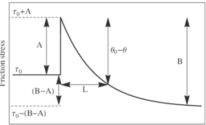
Fig. 3. A schematic illustration of the response to a step change in
the imposed velocity v of the spring block illustrated in Fig. 1. The imposed velocity, initially maintained constant at v0, is suddenly
in-cremented by 1v and subsequently held constant at v0+ 1v. The
friction stress τ , initially constant at τ0, suddenly increases to A
when the velocity is incremented by 1v and then decreases expo-nentially to a new value B. The length scale L characterizes the distance taken by the state variable θ to reach a new steady state θ0.
and t (for a discussion of non-dimensionalized variables, see also Gu et al., 1984). This non-dimensionalization puts the system into the following form:
˙θ = −v(θ + (1 + ǫ) log(v)) ˙u = v − 1 ˙v = −γ2[u + (1/ξ)(θ + log(v))] , (2)
where ǫ=(B−A)/A measures the sensitivity of the ve-locity relaxation, ξ=(kL)/A is the nondimensional spring constant, and γ=√k/M(L/vo) is the nondimensional
fre-quency. It is important to note that the parameter values cur-rently being used in the literature are approximately ǫ=3.1 (ǫ=1 in numerical simulations discussed in Rice and Tse, 1986), ξ=0.5 and γ =104− 1012(Madariaga, 1998).
The system has only one stationary solution, namely
(θ, u, v)=(0, 0, 1), which corresponds to steady sliding.
This solution is plotted in Fig. 4 under two different sets of parameter values. In this case, the numerical solution falls into its stationary state after a transient region and corre-sponds to no movement of the block relative to the driver plate. The block’s velocity is the same as that of the driver plate, thus its slip remains zero. Investigation of the local eigenvalues of system (2) will inform us as to what parameter combinations lead to bifurcations of the stationary solution, as well as how to choose a suitable numerical scheme. The Jacobian matrix Df is evaluated at the stationary solution to obtain matrix A: A= −1 0 −(1 + ǫ) 0 0 1 −γ2/ξ −γ2 −γ2/ξ
4 B. Erickson et al.: Aperiodic earthquakes
Fig. 4. Stationary solutions of system (2) whose parameter
val-ues have not crossed the Hopf bifurcation plane in Fig. 7. Here
(ǫ, ξ, γ )=(0.2, 0.8, 0.8) and (ǫ, ξ, γ )=(0.3, 1, 100) yield
station-ary solutions corresponding to no movement of the block relative to the driver plate. After a transient region, its velocity stays at a constant rate v=1 as it moves with the driver plate. Its relative slip is zero and its change in state (asperity contacts) is also zero.
The corresponding eigenvalues of A are computed and we find that the system has one non-zero real eigenvalue and a pair of complex conjugates, suggesting the possibility of a Hopf bifurcation to occur. When the matrix A has a sim-ple pair of pure imaginary eigenvalues and no other eigen-values with zero real part, then if the complex eigeneigen-values cross the imaginary axis, the stationary solution will undergo a Hopf bifurcation into a periodic orbit, see Guckenheimer and Holmes (1983) and Perko (2001) for more information about this bifurcation. Similar linearized stability analysis for rate and state dependent friction laws has been discussed by Gu et al. (1984) and Ranjith and Rice (1998).
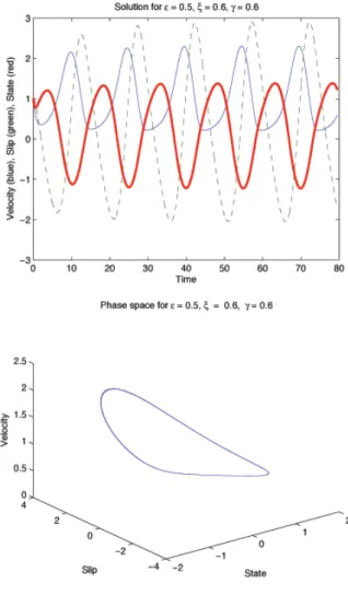
Fig. 5. Periodic solution of system (2) whose parameter values have
crossed the Hopf bifurcation plane (given by Fig. 7) and its associ-ated phase space. Here (ǫ, ξ, γ )=(0.5, 0.6, 0.6) yields a period one
orbit relatively smooth in its dynamics. The slip (green) fluctuates, increasing as the velocity (blue) peaks and decreasing as the ve-locity approaches zero. Similarly the state variable (red) decreases when the velocity peaks, but grows when the velocity reaches a min-imum, and the asperity contacts are reestablished. The correspond-ing phase portrait on the bottom is a smooth circular orbit where the periodicity between the velocity, slip and state is further clarified. Notice that the phase space is three-dimensional.
3 Numerical integration and analysis
In computing the local eigenvalues of Df at different times along a solution’s trajectory, we found that when the block’s velocity goes to zero (v→0), the minimum eigenvalue of Df is small (<<1) and decays exponentially towards−∞ as the parameter γ is increased. This is important to consider be-cause for commonly used values of γ (γ≈104−1012 accord-ing to Madariaga, 1998) the more negative the eigenvalue is, the stiffer the system will be. In regular systems, the choice
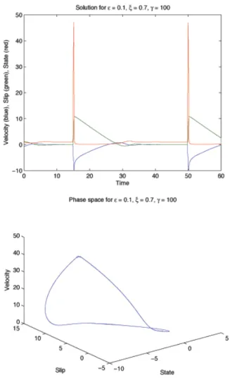
Fig. 6. Periodic solution of system (2) whose parameter values have
crossed the Hopf bifurcation plane (given by Fig. 7) and its associ-ated phase space. Here (ǫ, ξ, γ )=(0.1, 0.7, 100) yields a period one
orbit with similar dynamics to those in Fig. 5, but the changes in the velocity, slip and state are more sharp and distinguishable, corre-sponding to a more abrupt movement of the block relative to the driver plate. The associated phase portrait is also a circular orbit but not quite as smooth as that in Fig. 5. Notice that the phase space is three-dimensional.
of the time step should be chosen to satisfy accuracy re-quirements, and methods such as forward Euler and explicit Runge-Kutta methods can be used. In stiff systems, however, these explicit methods are numerically unstable and require very small time steps in order to maintain numerical stabil-ity. Implicit methods have the ability to remain stable even with larger time steps, thus we chose to use an implicit, sec-ond order backward-differentiation formula (BDF) numeri-cal scheme from Ascher and Petzold (1998), see appendix A for a summary of this method applied to system (2).
While the BDF scheme is stable, we find that the nonlin-earity of the logarithm term restricts our time step
nonethe-less. System (2) is stiff in time intervals where v approaches zero, i.e. if the step size is too large, then v can be com-puted to be negative (or zero). Evaluating log(v) at this time returns either an imaginary or undefined number and thus a completely inaccurate solution. If the step size is taken small enough, the velocity will move away from zero, due to the negative coefficient−γ2/ξ . Thus higher values of γ will
in-crease the stiffness in the system and require an extremely small time step. It appears that the time step 1t scales in-versely with γ (1t≈cγ−1 for some constant c), but no in-depth studies have been done on this.
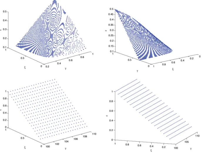
We have found that for small values of ǫ, stationary, period one and period two orbits result. In integrating this system numerically, solutions that were stationary undergo a Hopf bifurcation and periodic orbits are born. It is possible to cal-culate the parameter regions for which this bifurcation occurs as we have done in Fig. 7. Parameter combinations that lie below the surface will be stationary solutions, while combi-nations that lie above it will yield periodic solutions.
The first set of diagrams in Fig. 7 correspond to small val-ues of γ . The fact that it is a skewed surface means that a Hopf bifurcation is dependent on the values of all three pa-rameters. This result agrees with the analysis in Gu et al. (1984) where a transition to chaos was found by varying the parameter k. For higher values of γ , however, the Hopf bi-furcation surface takes the shape of a two-dimensional plane. Let us consider some simple trajectories in the parameter space illustrated in Fig. 7 with relevant consequences for the earthquake analogy. For fixed values of γ (i.e., fixed values of k and L), the trajectory for a Hopf bifurcation depends on
ǫ and ξ . In this case, we can observe a transition to chaos
by simply increasing the value of those two parameters (or equivalently the value of the parameters A and B) so as to cross the plane. This transition to chaos is thus independent of k and L, a result that differs from the results discussed in Gu et al. (1984), where they were not able to explore large values of k. Now consider the trajectories obtained by vary-ing the parameters (B−A) and A. In general, these trajec-tories are more complicated since both ǫ and ξ consequently vary. However, if the parameters k and L (used in the defini-tion of ξ ) are held constant, than ǫ is a linear funcdefini-tion of ξ , and the trajectories are straight lines again. For a large class of these trajectories, the lines will cross the Hopf bifurcation surface with a transition to chaos. These transitions are also independent of the values of k and L. In an earthquake anal-ogy to the single block, illustrated in Fig. 1, this suggests that potential transitions to chaos are essentially controlled by the ratio of the stress parameters (B−A) and A (see Fig. 3) and independent of the elastic property of the medium surround-ing the fault (idealized by the parameter k) and the critical length L of the friction law.
Figures 5 and 6 represent two period one orbits similar to that in Fig. 2. The solution in Fig. 5 is a periodic solu-tion but is more smooth in its mosolu-tion than that in Fig. 6 (or in Fig. 2), that represent more abrupt motion of the block
6 B. Erickson et al.: Aperiodic earthquakes
Fig. 7. Two Hopf Bifurcation Planes: Parameter spaces (from two different angles) for system (2) that yield a Hopf bifurcation. Parameter
combinations that lie below these surfaces will yield stationary solutions, while combinations above the two surfaces will yield periodic solutions. Top: Small values of γ produce a skewed surface in the (ǫ, ξ, γ ) plane while larger values of γ (bottom), produce a planar surface. In both cases, for a fixed γ and ξ , a Hopf bifurcation will occur when ǫ is sufficiently increased.
slipping beyond the driver plate. Initially the block is stuck on a rough surface so the relative slip to the driver plate de-creases at a constant rate as the driver plate catches up and even surpasses the block. Once the pulling force overcomes the static friction holding the block in place, the block’s ve-locity spikes, the slider shoots forward again and another cy-cle begins. The smoothness in the dynamics of Fig. 5 repre-sents a fluid-like interaction between the block and the rough surface it slides upon. The block fluctuates gently in response to the driver plate and the friction on the surface, but never completely sticks to it for any period of time. Note that when the velocity increases, the state variable decreases, a fact that supports the interpretation that the state variable measures the amount of contact the block has with the surface: when the block is stuck, the contacts will be greater than when the block is in motion. After the block arrests and comes to a
stop, the contacts begin to increase, a process that could be interpreted as fault healing after an event.
Periodic solutions can be viewed in the phase space, or by plotting the corresponding Poincar´e map as shown in the right of Fig. 8. The map is constructed by slicing a trans-verse hyperplane through the periodic solution in the phase space and taking a small neighborhood around the solution in the hyperplane (Guckenheimer and Holmes, 1983). Ex-plicitly, we sliced a plane in the phase space (θ, u, v), at
(θ, u, 1), generating a plot of where the periodic orbit crosses
the plane. Stationary solutions will, in general, not appear on the Poincar´e map. Period one orbits correspond to a fixed point of the Poincar´e map, period two orbits will appear as two points on the Poincar´e map etc., and chaotic orbits are represented by randomly distributed points on the map.
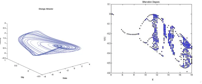
Fig. 8. Left: The strange attractor appears in the phase space of a single block after ǫ passes through a critical value. The attractor is a
compact set, invariant and with a neighborhood shrinking under the flow, to which orbits of the system approach. In our case, the attractor is an aperiodic orbit and that it is strange is determined by the system’s sensitive dependence on initial conditions, yielding broadband noise in the power spectrum. Right: Critical values of ǫ yield period doubling bifurcations of periodic orbits. The Poincar´e map is shown on the vertical axis, and the parameter ǫ on the horizontal axis.
Chaotic solutions to a spring-block model under a differ-ent rate and state dependdiffer-ent friction law have been seriously explored in Oancea and Laursen (1997), who studied bifur-cations of the system as they varied the pulling velocity at the end of the spring. As this velocity is increased, they found that growing oscillations would either become bounded peri-odic orbits or strange attractors, although periperi-odic windows would appear between the chaotic regimes. An attractor is a compact set in the phase space, invariant and with a neighbor-hood shrinking under the flow, to which orbits of the system are attracted. It is called a strange attractor if it exhibits sen-sitive dependence on initial conditions. See Guckenheimer and Holmes (1983) and Perko (2001) for more details on this topic.
Our system under Dieterich-Ruina style friction undergoes a sequence of period doubling bifurcations, until chaotic or-bits appear in the phase space, seen in the left of Fig. 8. These chaotic orbits are all pulled into an attractor in the phase space. If we consider the bifurcation diagram of the solution X(t )=(θ(t), u(t), v(t)) as a function of ǫ (viewed in the right of Fig. 8), then there is an initial interval where the attractor is a stationary solution. Then a Hopf bifurcation occurs and the attractor is a fixed point of the Poincar´e map corresponding to a periodic orbit of system (2). As seen in the right of Fig. 8, the system undergoes a Hopf bifurcation around ǫ≈4. Then a series of period doubling bifurcations occur and we get a sequence of intervals where the attractors are stable periodic orbits of period 4, 8, 16 etc. This period doubling cascade converges around ǫ=11.5, where a strange
attractor appears (Collet and Eckmann, 1980). If we assume that the nonlinear friction term in a single block system is responsible for simulating aperiodicity in earthquakes then it requires that ǫ be at least in this regime.
We can say a lot about the attractors of system (2) by studying the quadratic map, defined by the iterative equa-tion: xn+1=1−µxn2. Our simulations make it clear that
our Poincar´e map is in the same universality class as the quadratic map and exhibits the same bifurcations. The sys-tem defined by the quadratic map undergoes a period dou-bling bifurcation and becomes chaotic when µ>µcrit. Its
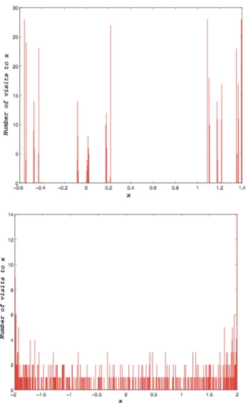
his-togram counts the number of times the chaotic orbit visits a given x value on the strange attractor. Figure 9 shows the histogram for two types of attractors for the quadratic map which will will discuss in more detail in the next two para-graphs to explain how to find signatures of aperiodicity.
From Fig. 8, one can see the period-doubling bifurcation points, ǫn, converge at ǫ∞, where limn→∞ǫn=ǫ∞≈11.5,
and the attractor becomes a singularly supported strange at-tractor with a histogram similar to that of the quadratic map, given in the top of Fig. 9. This means that the attractor con-sists of a thin set on the x-axis, where orbits visit only a set of points of Lebesgue measure zero. In each interval, the pe-riodic orbit from the previous interval survives, but becomes unstable. Thus each interval to the left of ǫ∞contains unsta-ble periodic orbits of all the previous periods. The histogram for the quadratic map can be compared with the histogram of slip on an earthquake fault. If the magnitude of slip is plotted against the number of slip events, and this data is compiled
8 B. Erickson et al.: Aperiodic earthquakes
Fig. 9. Histograms for a singularly supported attractor (top) and an
attractor with an absolutely continuous invariant measure (bottom). These figures are for the quadratic map. The x-axis is the interval where the map takes its values and the y-axis is the number of points that hit each x value (5000 points are sampled).
for sufficiently many earthquakes, one can obtain histograms that look similar to that in Fig. 9. This can be a guide in the analysis of earthquake data. Aperiodicity will appear in the histogram as either one of the strange attractors in Fig. 9, while periodicity will appear as isolated periodic peaks.
What can we say about the region beyond ǫ∞? It is known that the set of ǫ for which there exists no stable periodic orbit has positive Lebesgue measure, as does the slightly smaller set for which there is sensitive dependence on initial condi-tions. It has been proven more recently that the still smaller set where there exists absolutely continuous invariant mea-sures, living on support of the attractor on the x-axis, has positive Lebesgue measure. For these values of ǫ, the dy-namics reduce to ergodic theory on the strange attractor
us-ing the absolutely continuous invariant measure. In particular the ergodic theorem holds so we can exchange time averages by space averages (on the attractor) and the motion is mixing (Benedicks and Young, 1992), (Collet and Eckmann, 1980). This means that orbits on the strange attractor visit a dense set of points, as seen in the bottom of Fig. 9 (Benedicks and Young, 1992). For values of ǫ past 12, there are windows (open sets in ǫ) where the attractor returns to a periodic orbit from a chaotic one.
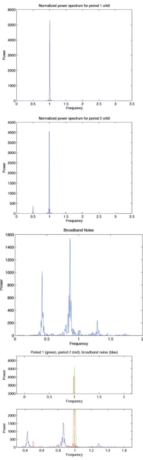
To confirm that the attractor is strange, we calculated the Fourier power spectrum for period 1, 2 and chaotic orbits, shown in Fig. 10. We took the numerical solution to the block’s slip, u(tn) at N discrete points, and computed its
dis-crete Fourier transform, ˆu(fk) for k=0, ..., N − 1. The
esti-mated power P (fk): =| ˆu(fk) ¯ˆu(fk)|/N2where fk : =k/1t
and ¯u is the conjugate of u (Press et al., 1986). The power spectrum will plot the mean squared amplitude of ˆu(fk)
against the positive frequencies fk for k=0, ..., N−1. After
normalizing the frequencies, the bifurcation from period one to period two is confirmed in the first two plots in Fig. 10. In the first plot, the single peak in power at frequency = 1 corre-sponds in period to one dominating Fourier coefficient in the Fourier expansion of the numerical solution. After the bifur-cation, a first peak appears at frequency = 12, i.e., double the period of the previous solution, and a second peak appears at frequency = 1, indicating a period two orbit. The broadband noise in the third plot in Fig. 10 indicates that the attractor is indeed strange (Berg´e et al., 1984), (Crutchfield et al., 1980) and the fourth figure plots the power of all three orbits so that the broadening of the spectrum can be well observed.
We briefly discuss the consequences of this transition to aperiodicity, with ǫ≈11.5, for the earthquake analogy of a single block. For this purpose, it should be noted that ǫ=1/S, where S is the non-dimensional seismic ratio introduced by Andrews (1976). In a paper discussing transition to super-shear velocity for the self-similar Dugdale model, Dunham (2007) observes that the crack tip will propagate at supers-hear velocity for S≈0.1 or smaller values. This range of S values corresponds to ǫ being on the order of 10 or larger (see Fig. 5 in Dunham, 2007). These results suggest that for the single block-faulting process, a sequence of aperi-odic earthquakes will be characterized by a rupture velocity that propagates at supershear velocity. Potential fault candi-dates for this model of aperiodicity include the San Andreas and the Kunlun faults (R. J. Archuleta, personal communi-cation, 2007). Finally, using the fault model computed by Archuleta (1984) for the 1979 Imperial Valley earthquake, Bouchon (1997) generates fault maps of the static stress drop and strength excess (Fig. 4 in Bouchon, 1997). Although the spatial distributions of the static stress drop and strength ex-cess are both heterogeneous, one can find regions of the fault where the ratio of the static stress drop to the strength excess is of the order of 10 and thus close to ǫ≈11.5.
Fig. 10. The Fourier power spectrum was taken for period 1,2 and
chaotic orbits. It plots the mean squared amplitude of the Fourier transform of the slip,ˆu(fk), against the positive frequencies fkfor
k=0, ..., N − 1. The bifurcation from period one to period two
is confirmed in the first two figures, and the broadband noise in the third figure suggests that the attractor is strange. The fourth figure plots the power of all three orbits so that the broadening of the spectrum can be well observed.
Fig. 11. Slip values of three different blocks for period two orbit
with ǫ= 0.51, ξ = 0.6, γ = 1.
4 The three block model
Systems of multiple blocks and springs have also been stud-ied in the past in an effort to better understand earthquake dynamics. Period-doubling and chaotic solutions have been observed in simulations of other earthquake models: two and three block models under velocity weakening friction were found to be quite complex if wider parameter ranges were studied (Galvanetto, 2002; De Sousa Vieira, 1999; Huang and Turcotte, 1990). In particular, Huang and Tur-cotte (1990) found that the system’s behavior was compara-ble to that of certain types of active faults, if studied over a wide parameter range. It is interesting to note that under Dieterich-Ruina style friction, as in our system, chaotic dy-namics resulted even with the use of one block. We explore a larger system to see where the threshold for chaos lies, and we find that chaotic dynamics emerge for smaller parameter values than those used in the single block system. We built
10 B. Erickson et al.: Aperiodic earthquakes
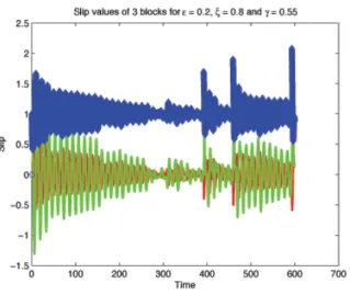
Fig. 12. Slip values of the three different blocks for an aperiodic
solution with ǫ=0.2, ξ=0.8, γ =0.55.
the three block system with Dieterich-Ruina friction and the equations of motion found in BK’s original paper.
We let xj represent the displacement from equilibrium of
the j t h block. Thus with µj+1as the spring constant
con-necting the j t h block to the j+1th block, and λj as the
spring constant connecting the j t h block to the driver plate, which is moving at a constant rate vo, our equations become:
mjx¨j=µj+1(xj+1−xj)−µj(xj−xj+1)−λj(xj−vot )+Fj,
for j =1, 2, 3. We have coupled the first and last block with a spring to make the system periodic and taken spring con-stants to be equal. We want to view the slip of the j t h block with respect to the driver plate, so we introduce the new variable: uj=xj−v0t . Thusu˙j=vj−v0where vj= ˙xj.
Re-writing as a non-dimensionalized set of first order equa-tions and applying the Dieterich-Ruina friction law (for Fj)
yields: ˙ θj=−vj(θj+(1+ǫ) log(vj)) ˙ uj=vj−1 ˙
vj=γ2[uj−1−2uj+uj+1−uj−(1/ξ)(θj+ log(vj))]
(3)
where the parameters, ǫ, ξ, γ remain those in Sect. 2, and all variables are non-dimensionalized versions of those in Eq. (2). We proceed by the computations preformed to the system in Sect. 2, first computing the Jacobian matrix for system (3) evaluated at its stationary solution and finding its associated eigenvalues.
We notice that if we increase the same parameter ǫ, and strongly couple the blocks so that they are not allowed to move very independently, (i.e. we set ξ=0.6), then the sys-tem undergoes a similar bifurcation from a stationary solu-tion to a periodic orbit as the one block system. Some further
exploration into parameter combinations leads to a period two orbit. The important difference from the single degree of freedom model (2) is that these period doublings occur for a range of parameter values comparable to those derived in the laboratory. Figure 11 shows a plot for parameters on the order of 10−1, i.e., a much smaller value than for the single block. When ǫ is further increased we find aperiodic orbits like that in Fig. 12 and conclude that for the system of three blocks, the threshold for chaos is greatly lowered for values of ξ and ǫ. The route to chaos for very large values of γ remains an open question.
5 Conclusions
We have shown that the single degree of freedom block and spring model (2) with the Dieterich-Ruina friction law ex-hibits complex behavior. By using the full nonlinearity of the friction term, we see that for a set of parameter values, the system remains in a stationary state. An increase in the parameter ǫ forces the system to undergo a Hopf bifurcation from a stationary solution to a periodic orbit, some of which exhibit stick slip behavior reminiscent of earthquake dynam-ics. The periodic orbit then undergoes a period doubling bi-furcation initiating a period doubling cascade where we find periodic orbits of period 2, 4, 8, 16 etc. When ǫ reaches
ǫ∞, the periodic orbit bifurcates into an aperiodic orbit on a singularly supported strange attractor. Past ǫ∞, there exists absolutely continuous invariant measures living on support of the attractor and we find windows in which periodic orbits appear and then bifurcate into aperiodic orbits.
The transition to complex behavior discussed in this paper is determined by the parameter ǫ. This parameter is indepen-dent of the characteristic length scale L, suggesting that com-plex behavior should be observed irrespectively of the value taken by L. This is an important result in view of the current debate over the question of using laboratory derived values of L in numerical computations of the earthquake rupture model (Lapusta and Rice (2003), for example). According to Fig. 3, the parameter ǫ quantifies the balance between the final friction stress increment given by (B−A) and the stress increment A due to the sudden jump in the imposed velocity
1v. Translated to earthquake motion, this picture suggests
that the parameter ǫ is principally determined by the ratio of the amount of “stress” dropped during an earthquake to the increase in stress that accompanies the sudden change in the fault velocity. Provided that the former is sufficiently large when compared to the latter, the parameter ǫ will be large enough to ensure that a sequence of earthquake motions will be in the chaotic regime. A similar conclusion can be held regarding the parameter k corresponding to the linear elas-tic properties of the medium surrounding the fault (Gu et al., 1984).
The periodic model for the recurrence of large earthquakes has been largely developed by Reid (1910), however support
for this idea lacks empirical evidence. (For a detailed dis-cussion of the concept of periodic earthquakes see Scholz, 2002 – Fig. 5.34 in this book is a schematic illustration sim-ilar to the one block system in Fig. 1). Furthermore, tran-sitions to chaos have been observed for the simple configu-ration of two or three coupled blocks (Huang and Turcotte, 1990; De Sousa Vieira, 1999; Galvanetto, 2002). In this pa-per we showed that even for a single block with a nonlinear friction law, a transition to chaos can be observed. The anal-ogy with earthquake motion suggests that the friction law can be a potential source for the observation of aperiodicity in earthquake dynamics (Huang and Turcotte, 1990).
It is important to note that non-periodic behavior ob-served in this simple problem may be partially responsible for irregular ground motion in addition to the heterogeneity in the stress distribution as simulated in Lapusta and Rice (2003). Furthermore, it will be important to see how this non-periodic behavior will affect the nucleation process in the numerical simulation of sequences of earthquakes. Our results suggest that the use of the nonlinear friction term gen-erates chaotic regimes that approximations to the term may not produce. There are also empirical results from the labo-ratory, obtained by Drummond (1999), whose friction mea-surements suggest the presence of a strange attractor. Be-cause it is possible to calculate the stiffness of system (2) at different times, a stiff solver seems to be the method of choice given high values of γ for which an extremely small time step is required. Rather than regularize the nonlinear friction term as done previously in Lapusta and Rice (2003) and Szkutnik et al. (2003), it is possible to numerically in-tegrate the system without an approximation to the friction term. Although we cannot yet study the bifurcations of solu-tions for higher values of γ , it is possible to calculate param-eter spaces for which Hopf bifurcations occur and dparam-etermine the chaotic regimes for this system.
Appendix A
Backward Differentiation Formula (BDF):
The BDF method solves the differential equation: y′=f(t, y). It is derived by taking a second order approximation to y′by:
y′≈ 3yn− 4yn−1+ yn−2 2h
Given the initial condition, y1, one step of backward Euler is
done to obtain y2and the BDF scheme is ready to be
imple-mented:
3yn− 4yn−1+ yn−2= 2hf(tn, yn)
Since f(t, y) is usually a nonlinear function, we rewrite the scheme as:
3yn− 4yn−1+ yn−2− 2hf(tn, yn)= 0
and at every time step, apply Newton’s method to solve the root problem.
For every fixed step in time, n, the yνn+1thiteration under Newton’s method is given by:
yνn+1= yνn− (3I − 2hDf(tn, yνn))−1
(3yνn− 4yn−1+ yn−2− 2hf(tn, yνn)),
where the vectors yνnand f(tn, yνn) are given by,
yνn= θnν uνn vνn f(tn, yνn)= −vν n(θnν+ (1 + ǫ)log(vνn)) vνn− 1 −γ2(uν n+ (1/ξ)(θnν+ log(vνn))
and the matrix Df(tn, yνn) is
Df= −vν n 0 −θnν− (1 + ǫ)(log(vνn)+ 1) 0 0 1 −γ2/ξ −γ2 (−γ2/ξ )(1/vν n)
Acknowledgements. The authors were supported by grants number
DMS-0352563 from the National Science Foundation whose support is gratefully acknowledged. We would like to thank Alethea Barbaro and Eric Daub at UCSB as well as R. J. Archuleta and J. C. Nave for their insight and helpful suggestions. We would also like to thank G. O. Mohler at UCSB for his advice on numerical methods used for this paper. We would like to thank Raul Madariaga and the second anonymous reviewer for their comments and suggestions. This research has been supported by LANL/IGPP grant No. 04-08-16L-1532 and by the Southern California Earth-quake Center. SCEC is funded by NSF Cooperative Agreement EAR-0106924 and USGS Cooperative Agreement 02HQAG0008. This is SCEC Contribution No. 1133. This is ICS contribution No. 0814.
Edited by: G. Zoeller
Reviewed by: R. Madariaga and another anonymous referee
References
Andrews, D. J.: Rupture velocity of plane strain shear cracks, J. Geophys. Res., 81, 5679–5687, 1976.
Ascher, U. M. and Petzold, L. R.: Computer methods for ordi-nary differential equations and differential-algebraic equations, SIAM, Philadelphia, 1st edition, 1998.
Archuleta, R. J.: A faulting model for the 1979 Imperial Valley earthquake, J. Geophys. Res., 89, 4559–4586, 1984.
Bak, P., Tang, C., and Wiesenfeld, K.: Self-organized criticality: an explanation of 1/f noise, Phys. Rev. Lett., 59, 381–384, 1987. Bak, P., Tang, C., and Wiesenfeld, K.: Self-organized criticality,
Phys. Rev. Lett., 38, 364–374, 1988.
Beeler, N. M., Lockner, D. L., and Hickman, S. H.: A simple stick-slip and creep-stick-slip model for repeating earthquakes and its impli-cation for microearthquakes at parkfield, Bull. Seism. Soc. Am., 91, 1797–1804, 2001.
12 B. Erickson et al.: Aperiodic earthquakes Benedicks, M. and Young, L.: Absolutely continuous invariant
measures and random perturbations for certain one-dimensional maps, Ergod. Th. and Dynam. Sys., 12, 13–37, 1992.
Berg´e, P., Pomeau, Y., and Vidal, C.: Order within chaos: towards a deterministic approach to turbulence. Herman, Paris, 1st edition, 1984.
Bouchon, M.: The state of stress on some faults of the San An-dreas system as inferred from near-field strong motion data, J. Geophys. Res., 102, 11 731–11 744, 1997.
Burridge, R. and Knopoff, L: Model and theoretical seismicity, Bull. Seism. Soc. Am., 57, 341–371, 1967.
Carlson, J. M. and Batista, A. A.: Constitutive relation for the fric-tion between lubricated surfaces, The American Physical Soci-ety, 53, 4153–4165, 1996.
Carlson, J. M., Langer, J. S., and Shaw, B. E.: Dynamics of Earth-quake Faults, Rev. Modern Phys., 66, 657–670, 1994.
Clancy, I. and Corcoran, D: Criticality in the burridge-knopoff model, Phys. Rev. R, 71, 335–339, 2005.
Collet, P. and Eckmann, J. P.: Iterated maps on the interval as dy-namical systems, Birkhauser, Philadelphia, 1st edition, 1980. Crutchfield, J., Farmer, D., Packard, N., Shaw, R., Jones, G., and
Donelly, R.J.: Power spectral analysis of a dynamical system, Phys. Lett. A, 76,1–4, 1980.
De Sousa Vieira, M.: Chaos and synchronized chaos in an earth-quake model, Phys. Rev. Lett., 82, 201–204, 1999.
Dieterich, J. H. and Kilgore, B. D.: Direct observation of frictional contacts: new insights for state dependent properties, Pure Appl. Geophys., 143, 283–302, 1994.
Drummond, C.: Nanotribology of confined thin films, Ph.D, Uni-versity of California at Santa Barbara, Santa Barbara, CA, 1999. Dunham, E. M.: Conditions governing the occurence of supershear rupture under slip weakening friction, J. Geophys. Res., 112, B07302, doi:10.1029/2006JB004717, 2007.
Galvanetto, U.: Some remarks on the two-block symmetric Burridge-Knopoff model, Phys. Lett. A, 293, 251–259, 2002. Gross, S.: Traveling wave and rough fault earthquake models:
il-luminating the relationship between slip deficit and event fre-quency statistics, Am. Geophys. Union, 88, 10 359–10 370, 2000.
Gu, J-C., Rice, J. R., Ruina, A. L., and Tse, S. T.: Slip motion and instability of a single degree of freedom elastic system with rate and state dependent friction, J. Mech. Phys. Solids, 32, 167–196, 1984.
Guckenheimer, J. and Holmes, P.: Nonlinear oscillations, dynam-ical systems, and bifurcations of vector fields, Springer-Verlag, New York, 1st edition, 1983.
Huang, J. and Turcotte, D. L.: Evidence for chaotic fault inter-actions in the seismicity of the San Andreas fault and Nankai trough, Nature, 348, 234–236, 1990.
Kanamori, H. and Anderson D. L.: Theoretical basis of some empir-ical relations in seismology, Bull. Seismol. Soc. Am., 65, 1073– 1095, 1975.
Lapusta, N. and Rice, J. R.: Nucleation and early seismic propaga-tion of small and large events in a crustal earthquake model, J. Geophys. Res., 108, 1–18, 2003.
Madariaga, R.: Study of an oscillator of single degree of free-dom with dieterich-ruina rate and state friction, Laboratoire de G´eologie, Ecole Normale Sup´erieure, Unpublished Notes (Preprint), 1998.
Marone, C.: Laboratory-derived friction laws and their application to seismic faulting, Annu. Rev. Earth Planet. Sci., 26, 643–696, 1998.
Oancea, V. G. and Laursen, T. A.: Stability analysis of state depen-dent dynamic frictional sliding, Int. J. Non-Linear Mechanics, 32, 837–853, 1997.
Ohnaka, M. and Shen, L.-F.: Scaling of the shear rupture process from nucleation to dynamic propogation: implications of geo-metric irregularity of the rupturing surfaces, J. Geophys. Res., 104, 817–844, 1999.
Pelletier, J. D.: Spring-block models of seismicity: review and anal-ysis of a structurally heterogeneous model coupled to a viscous asthenosphere, Geophysical Monograph, 120, 27–42, 2000. Perko, L.: Differential equations and dynamical systems,
Springer-Verlag, New York, 3rd edition, 2001.
Press, W. H., Teukolsky, S. A., Vetterling, W. T., and Flannery, B. P.: Numerical recipes in fortran, Cambridge University Press, New York, 2nd edition, 1986.
Ranjith, K. and Rice, J. R.: Stability of quasi-static slip in a single degree of freedom elastic system with rate and state dependent friction, citeseer.ist.psu.edu/496282.html, 1998.
Reid, H. F.: The mechanism of the earthquake, the california earth-quake of April 18, 1906, Report of the state earthearth-quake investi-gation commission, Vol. 2. Washington DC: Carnegie Institution, 1910.
Rice, J. R.: Constitutive relations for fault slip and earthquake in-stabilities, Pure Appl. Geophys., 121, 443–475, 1983.
Rice, J. R. and Tse, S. T.: Dynamic motion of a single degree of freedom system following a rate and state dependent friction law, J. Geophys. Res., 91, 521–530, 1986.
Rice, J. R., Lapusta, N., and Ranjith, K.: Rate and state depen-dent friction and the stability of sliding between elastically de-formable solids, J. Mech. Phys. Solids, 49, 1865–1898, 2001. Ruina, A.: Slip instability and state variable friction laws, J.
Geo-phys. Res., 88, 10 359–10 370, 1983.
Shkoller, S. and Minster, J. B.: Reduction of dietrich-ruina attrac-tors to unimodal maps, Nonlin. Processes Geophys., 4, 63–69, 1997,
http://www.nonlin-processes-geophys.net/4/63/1997/.
Scholz, C. H.: The mechanics of earthquakes and faulting, Cam-bridge University Press, CamCam-bridge, 2nd edition, 2002. Szkutnik, J., Kawecka-Magiera, B., and Kulakowski, K.:
History-dependent synchronization in the burridge-knopoff model, http://www.citebase.org/abstract?id=oai:arXiv.org:nlin/ 0310030, 2003.
Turcotte, D. L and Malamud, B. D.: International Handbook of Earthquake and Engineering Seismology, Academic Press, San Diego, Chapter 14, 2002.
USGS: Earthquake hazards program northern california, http:// quake.usgs.gov/research/parkfield/repeat.html, 2002.