Efficiently and Effectively Answering Why-Not Questions based on Provenance Polynomials

HAL Id: hal-01131561

https://hal.inria.fr/hal-01131561

Submitted on 14 Mar 2015

HAL is a multi-disciplinary open access

archive for the deposit and dissemination of

sci-entific research documents, whether they are

pub-lished or not. The documents may come from

teaching and research institutions in France or

L’archive ouverte pluridisciplinaire HAL, est

destinée au dépôt et à la diffusion de documents

scientifiques de niveau recherche, publiés ou non,

émanant des établissements d’enseignement et de

recherche français ou étrangers, des laboratoires

Questions based on Provenance Polynomials

Nicole Bidoit, Melanie Herschel, Katerina Tzompanaki

To cite this version:

Nicole Bidoit, Melanie Herschel, Katerina Tzompanaki. Efficiently and Effectively Answering

Why-Not Questions based on Provenance Polynomials. [Research Report] RR-8697, OAK team, Inria

Saclay; INRIA. 2015, pp.25. �hal-01131561�

0249-6399 ISRN INRIA/RR--8697--FR+ENG

RESEARCH

REPORT

N° 8697

Efficiently and Effectively

Answering Why-Not

Questions based on

Provenance Polynomials

RESEARCH CENTRE SACLAY – ÎLE-DE-FRANCE

1 rue Honoré d’Estienne d’Orves Bâtiment Alan Turing

Campus de l’École Polytechnique

Questions based on Provenance Polynomials

Nicole Bidoit, Melanie Herschel

_{, Katerina Tzompanaki}

Project-Teams OAK

Research Report n° 8697 — March 2015 — 25 pages

Abstract: The problem of answering Why-Not questions consists in explaining why the result of a query does not contain some expected data, i.e., missing answers. To solve this problem, we resort to identifying where in the query, data relevant to the missing answer were lost. Existing algorithms producing such query-based explanations rely on a query tree representation, potentially leading to different or partial explanations. This significantly impairs on the effectiveness of computed explanations. Here we present an effective, query-tree independent representation of query-based explanations, for a wide class of Why-Not questions, based on provenance polynomials. We further describe an algorithm that efficiently computes the complete set of these explanations. An experimental evaluation validates our statements.

Key-words: Why-Not questions, data provenance

des polynômes de provenance

Résumé : Une question de type "pourquoi pas" (Why Not) exprime une interrogation relative à l’absence dans le résultat d’une requête de certaines réponses attendues par l’utilisateur. Donc répondre à des ques-tions de type "pourquoi pas" consiste à fournir une explication relative à l’absence de réponses. La solu-tion que nous proposons cherche à identifier les éléments de la requête responsables de la perte de données ayant pu potentiellement contribuer à construction de ces réponses attendues mais manquantes. Les algo-rithmes existants qui produisent ce type d’explication dite "explication par la requête" sont développés en s’appuyant sur une représentation de la requête par un arbre. Cette approche a pour conséquence de pro-duire des explications qui sont partielles d’une part et qui dépendent de l’arbre de requête choisi d’autre part. Celle-ci nuit donc à la qualité de l’explication. Dans cet article, nous proposons une méthode qui résoud, pour une classe de requêtes très grande, le défaut des travaux antérieurs en produisant des expli-cations sous forme de polynômes de conditions inspirée par les polynômes de provenance. Un algorithme efficace est développé qui permet de calculer ces explications. La méthode est validée par cet algorithme et des expérimentations pertinentes.

SELECT island, archipel FROM Island I,

Archipelago A WHERE I.AID = A.AID AND pop <= 20M

Island

island pop AID

M aui 144K 1 Hawaii 3187K 1 Reunion 841K 2 M adagascar 22M NULL Archipelago AID archipel 1 Hawaii 2 M ascarene

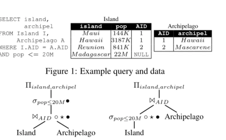
Figure 1: Example query and data

Πisland,archipel σpop≤20M• 1AID◦ ? • Island Archipelago Πisland,archipel 1AID σpop≤20M◦ ? • Island Archipelago

Figure 2: Reordered query trees for the query of Fig. 1 and algorithm results (Why-Not ◦, NedExplain ?, Conseil •)

1 Introduction

The increasing load of data produced nowadays is coupled with an increasing need for complex data transformations that developers design to process these data in every-day tasks. These transformations, commonly specified declaratively, may result in unexpected outcomes. For instance, given the query and data of Fig. 1, a developer (or scientist) may wonder why the island of Madagascar is missing from the result, even though she expected it to be part of it. Traditionally, she would repeatedly manually analyze the query to identify a possible reason, fix it, and test it to check whether the missing answer is now present or if other problems need to be fixed.

Answering such Why-Not questions, that is, understanding why some data are not part of the result, is very valuable in a series of applications, such as query development, query debugging, query refinement, or what-if analysis. To help developers explain missing answers, different algorithms have recently been proposed for relational and SQL queries [5, 7, 14, 16, 17] as well as other types of queries (top-k [13], reverse skyline queries [19]). In this paper, we focus on relational queries, for which existing algorithms explain a missing answer either based on the data (instance-based explanations), the query (query-based explanations), or both (hybrid explanations). Moreover, we focus on solutions producing query-based ex-planations, as these are generally more efficient while providing sufficient information for query analysis and debugging. Taking a closer look at existing methods, we notice that these return different explana-tions for the same SQL query. This is due to the fact that these algorithms are designed over query trees rather than over the query, and thus trace data relevant to the missing answer, i.e., compatible data in a bottom-up manner through a specific query tree from which so-called picky operators are identified. Example 1.1 Consider the SQL query q and data I of Fig. 1 and assume that a developer wants an explanation for the absence of island Madagascar in the query result q(I). So here, the why-not question is “Why is tuple (island:Madagascar, archipel:x) not in q(I)?”. Fig. 2 shows two possible query trees for q. It also shows the picky operators that Why-Not [7] (◦) and NedExplain [5] (?) return as query-based explanations as well as query operators returned as part of hybrid explanations by Conseil [14] (•). Each algorithm returns a different result for each of the two query trees, and in most cases, it is only a partial result as the true explanation of the missing answer is that both the selection is too strict for the compatible tuple (Madagascar, 22M, NULL) from table Island and this tuple does not find any join partner in table Archipelago.

The above example clearly shows that existing algorithms have limited effectiveness when it comes to explaining missing answers. Indeed, the developer first has to understand and reason at the level of query trees instead of reasoning at the level of the declarative SQL query she is familiar with. Second,

she always has to wonder whether the explanation is complete. To provide a more informative Why-Not answer we present in this paper the Why-Not answer in form of a polynomial. We then discuss both a naive and an efficient algorithm to compute this answer. Thus, the overall contribution of this paper is both an efficient and effective way to answer Why-Not questions for relational queries using provenance polynomials. In detail, our contributions are1_:

Why-Not answer polynomial. Our formal framework supports a larger class of Why-Not questions w.r.t. previous works. The form of the Why-Not answer is unprecedented, as this paper is the first to formalize provenance polynomials providing fine-grained query based explanations. Intuitively, each addend of a polynomial represents one combination of the query conditions that simultaneously explain the missing answers and the set of all addends covers all possible such combinations. Moreover, the Why-Not answer is independent of the query tree representation of a query q. More precisely, all query trees which are equivalent to a conjunctive query (possibly) containing inequalities and which are obtained from each other by reordering of the operators have the same Why-Not answer polynomial up to isomorphism. Naive Ted algorithm and efficient Ted++ algorithm. We present the Ted algorithm that correctly com-putes the Why-Not answer polynomial for a given query and a given Why-Not question. However, we show that its runtime complexity is impractical. Thus, we subsequently present an improved algorithm, Ted++, that is capable of efficiently computing the same Why-Not answer polynomial.

Experimental validation. We validate both the efficiency and the effectiveness of the solutions proposed in this paper through a series of experiments. These experiments include a comparative evaluation to existing algorithms computing query-based explanations for SQL queries (or sub-languages thereof) as well as a thorough study of Ted++ performance w.r.t. different parameters.

The remainder of this paper is structured as follows. Sec. 2 covers related work. Sec. 3 defines in detail our problem setting and the novel Why-Not answer polynomials. We briefly cover the naive Ted algorithm in Sec. 4 before we discuss in more detail the efficient Ted++ algorithm in Sec 5. We present our experimental setup and evaluation in Sec. 6 before we conclude in Sec. 7.

2 Related Work

Recently, we observe the trend that growing volumes of data are processed by programs developed not only by expert developers but also by less knowledgable users (creation of mashups, use of web services, etc.). These trends have led to the necessity of providing algorithms and tools to better understand and verify the behavior and semantics of developed data transformations, and various solutions have been proposed so far, including data lineage [9] and more generally data provenance [8], (sub-query) result in-spection and explanation [11, 25], query conditions relaxation [23], visualization [10], or transformation specification simplification [20, 24]. The work presented in this paper falls in the category of data prove-nance research, focusing on a specific sub-problem that aims at explaining missing answers from query results. This sub-problem alone finds applications in various domains, e.g., information extraction [17], query debugging [15], distributed systems debugging [27], or image retrieval [3].

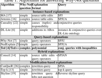
Due to the lack of space, the subsequent discussion focuses on algorithms proposed for answering Why-Not questions. Tab. 1 summarizes these approaches, first classifying them according to the type of explanation they generate (instance-based, query-based, hybrid, or modification-based). The table further shows whether an algorithm supports simple Why-Not questions, i.e., questions where each condition impacts one relation only, or more complex ones. The last two columns summarize the form of a returned explanation and the queries an algorithm supports, respectively.

1_{In a four-page workshop paper [4], we introduced the Why-Not answer polynomial as well as the naive Ted algorithm. Opposed}

to the workshop paper, the definitions here are more concise and additional theorems have been added. We also briefly summarize Ted here to clearly show that it is impractical, however, the focus of this paper clearly lies on the presentation of Ted++. Finally, the workshop paper does not include any experiments.

Table 1: Algorithms for answering Why-Not questions Algorithm Why-NotExplanation Query

question format

Instance-based explanations MA [17] simple source table edits SPJ Artemis [16] complex source table edits SPJUA Causality [22] simple causes (tuples) and

responsibility conjunctive queries

DL-Lite [6] simple additions to ABox instance & conjunctive queries over DL-Lite ontology

Query-based explanations Why-Not [7] simple query operators SPJU NedExplain [5]simple query operators SPJUA

Ted [4]/Ted++ complex polynomial conj. queries with inequalities Hybrid explanations

Conseil [14] simple source table edits + query operators SPJAN Modification-based explanations ConQueR [26] complex rewritten query SPJA Top-k [13] simple rewritten query top-k query Skyline [19] simple rewritten query &

why-not question Reverse skyline query

Instance-based explanations. Both Missing-Answers (MA) [17] and Artemis [16] compute instance-based explanations in the form of source table edits (insertions or updates) that would be necessary to obtain the missing answers in the query result. Whereas MA returns correct explanations for simple Why-Not questions and SQL queries involving selection, projection, and join only (SPJ queries), Artemis supports complex why-not questions on a larger fraction of SQL queries (including union or aggregation, denoted SPJUA). Causality [22] theoretically studies the unification of instance-based explanations of missing answers and of data present in a query result, leveraging the concepts of causality and responsi-bility. The results apply to conjunctive queries. Finally, DL-Lite [6] leverages abductive reasoning and theoretically examines the problem of computing instance-based explanations for a class of simple Why-Not questions on data represented by a DL-Lite ontology. Here, the instance-based explanation consists in additions to the ontology’s ABox (insertions to the instance data).

Query-based and hybrid explanations. Why-Not [7] takes as input a simple Why-Not question and returns so called picky query operators as query-based explanation. To determine these, the algorithm first identifies tuples in the source database that satisfy the conditions of the input Why-Not question and that are not part of the lineage [9] of any tuple in the query result. These tuples, named compatible tuples, are traced through the query operators of a query tree representation to identify which operators include them in their input but not in their output. In [7] the algorithm is shown to work for queries involving selection, projection, join, and union (SPJU query). NedExplain [5] is very similar to Why-Not in the sense that it supports simple Why-Not questions and returns a set of picky operators as query-based Why-Not answer as well. However, it supports a broader range of queries, i.e., queries involving selection, projection, join, and aggregation (SPJA queries) and unions thereof and the computation of picky operators is significantly different. First, it does not restrict compatible tuples to source tuples not in the lineage of any result tuple. Second, based on a novel formal definition of query-based explanations, NedExplain computes a generally wider and detailed set of explanations than Why-Not.

Conseil [14] produces hybrid explanations that include an instance-based component (source table edits) and a query-based component. The latter consists in a set of picky query operators. However, as Conseil considers both the data to be possibly incomplete and the query to be possibly faulty, the set of picky query operators associated to a hybrid explanation depends on the set of source edits of the same hybrid explanation. In general, this results in Conseil returning multiple hybrid explanations where the sets of picky operators of each explanation are different from those determined by Why-Not or NedExplain.

For comparison purposes, Tab. 1 also includes the naive Ted algorithm (previously introduced in a short workshop paper [4]) and Ted++. We observe that it is the first algorithm that computes

query-based explanations for complex Why-Not questions, along with the novel format of Why-Not answer polynomial. Finally, Ted++ applies on a different query fragment than the two previous algorithms, i.e., conjunctive queries with inequalities.

Modification-based explanations. Given a set of missing answers, an SPJUA query, and a source database, ConQueR [26] rewrites the query such that all missing answers become part of the output. Beyond SQL queries, the Top-K algorithm [13] focuses on changing k or preference weights to make the missing answer appear in the query result of a top-k query. Skyline [19] presents a solution for answering Why-Not questions in reverse skyline queries that modifies not only the query, but also the Why-Not question itself. Although these approaches are very interesting and valuable for the general purpose of query refinement, they are out of the scope of this paper.

3 Why-Not answers as Polynomial

We assume the reader is familiar with the relational model [1]. We briefly revisit certain notions in our context in Sec. 3.1. Why-Not questions are defined in Sec. 3.2. Sec. 3.3 extends the notion of compatible data introduced in previous work. Finally, we define the answer of a Why-Not question in Sec. 3.4 and discuss interesting properties in Sec. 3.5.

3.1 Preliminaries

We assume that a database schema S is a set of relation schemas. The set of attributes of a relation

Ralways includes a special attribute R_Id because we assume that each tuple in an instance of R is

referred to by an identifier Id. We denote by Att(R) the set of attributes of R, except R_Id. We assume each attribute of R to be qualified, i.e., of the form R.A. For an instance I over S, we write I|Rfor the component of I over R. We also assume available a set V ar of variables x, y, z, . . . A condition c is either of the form xθy or xθa, where x, y∈V ar, a is a constant in a unique domain D and θ∈{=, 6=, <, ≤}. A v-tuple v over R is a tuple of pairwise distinct variables over Att(R). Note that a v-tuple does not associate a variable with the attribute R_Id. Next, var(·) is used to retrieve the set of variables from a structure, e.g., var((x1, . . . , xn))returns {x1, . . . , xn}. The paper uses a notion of queries close to that of tableaux [2] and of inequality queries [21].

Definition 3.1 (Query tableau) A query tableau (or simply query) q over schema Sqis a triple (sq, Tq, Cq) where (i) the summary sqis a set of distinguished variables with sq⊆var(Tq), (ii) the query skeleton Tqis a mapping associating one v-tuple v to each R∈Sqsuch that var(Tq(R))∩var(Tq(T )=∅for any distinct pair R, T ∈Sq, and (iii) the query condition Cq is a set of conditions over var(Tq).

To denote the result of q over I, we use q(I). Note also that our query definition does not allow express-ing conditions involvexpress-ing the special attribute R_Id. These attributes thus do not appear in the tableau representation. Next, if a condition c in Cq refers via its variables to two distinct relations, we say that c is a complex condition, otherwise c is a simple condition.

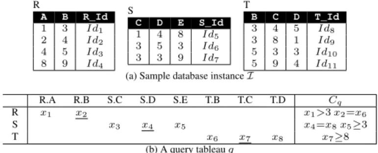
Example 3.1 Consider the database schema Sq={R, S, T }. Fig. 3 displays an instance I of Sqand the tableau representing a query q. The distinguished variables for q are underlined and the query condition is given in a special column. This query q corresponds to the following relational query:

πR.B,S.D,T.C(σR.A>3[R]1BσT.C≥8[T ]1DσS.E≥3[S])

The condition x2=x6is complex because the variables x2, resp. x6refer to R, resp. T . The condition x4=x8is complex as well. All other conditions are simple ones.

3.2 The Why-Not Question

Given a quey q, a Why-Not question is in general formulated as a predicate that is a disjunction of conditional tuples (c-tuples) [18]. Next, w.l.o.g., we concentrate on predicates composed of a single c-tuple. A full definition is available in [5]. The method presented here trivially extends to general predicates, but we omit a discussion due to space limitation.

Definition 3.2 (Why-Not question) Let q=(sq, Tq, Cq)be a query over Sq. A (simple) Why-Not ques-tion is specified by a c-tuple tc=(tv,Vni=1ci), where (i) tvis a tuple of variables such that var(tv)⊆var(sq), and (ii) ciis a condition over the variables var(tv). Next, tc.conddenotes Vni=1ci. A Why-Not question tcis complex if one of its condition is complex, ortherwise it is simple.

Example 3.2 Given the scenario of Ex. 3.1, we wonder why, in the answer q(I), there is no tuple s.t. the value on R.B is smaller than the one on S.D and at the same time its value on T.C is smaller or equal to 9. This Why-Not question is expressed by tc=((x2, x4, x7), (x2<x4∧ x7≤9)). In tc.cond, x7≤9is a simple condition whereas x2<x4is a complex one. Consequently, tcis a complex c-tuple.

3.3 Compatible Data

Intuitively, compatible data designates any source tuples that potentially provide data to build the missing answer specified by tc. The first step towards answering the Why-Not question consists in identifying, in the input instance I, these tuples and more specifically combinations of them (called concatenated tuples) that would produce the missing answer in the absence of the restrictions of q. In a second step, discussed in the next section, we will identify the conditions in q that prune these concatenated tuples.

Example 3.3 One can note in tc.condof Ex. 3.2, that a missing answer depends on those tuples tR∈I|R, tS∈I|S and tT∈I|T that satisfy tR(R.B)<tS(S.D)and tT(T.C)≤9. Due to the complex condition, tR and tS need to be chosen in correlation with one another, whereas it is not the case for tT. Thus, here the compatible concatenated tuples correlated with (tR, tS)are (Id1Id5), (Id1Id6)and (Id2Id6), while for tT, each tuple in S, i.e., Id8, . . . , Id11, is a compatible concatenated tuple.

Previous approaches [5, 7] generate compatible tuples independently from each other, e.g., both Id1 and Id2are considered compatible for tR. However, Id2should not be considered compatible when Id5 is chosen for tS, which is not addressed by previous work. Therefore, we introduce compatibility on con-catenated tuples rather than on single tuples. According to our definition, each compatible concon-catenated tuple (cc-tuple) would produce a missing answer tuple if it was not pruned by some condition(s) of the query.

Mappings. For a concise presentation, we need the functions defined and illustrated in Tab. 2. Function hAttis extended to apply on the tableau and the c-tuple conditions respectively, whereas function full naturally extends to cc-tuples, e.g., full(Id1Id5)=(R.A:1, R.B:3, S.C:1, S.D:4, S.E:8).

R A B R_Id 1 3 Id1 2 4 Id2 4 5 Id3 8 9 Id4 S C D E S_Id 1 4 8 Id5 3 5 3 Id6 3 3 9 Id7 T B C D T_Id 3 4 5 Id8 3 8 1 Id9 5 3 3 Id10 5 9 4 Id11

(a) Sample database instance I

R.A R.B S.C S.D S.E T.B T.C T.D Cq

R x1 x2 x1>3 x2=x6

S x3 x4 x5 x4=x8x5≥3

T x6 x7 x8 x7≥8

(b) A query tableau q

Table 2: Mapping functions

Function Purpose Example

hAtt:Att(Sq)→ var(T_Sq) Maps attribute names to

vari-ables in Tq.

hAtt(R.A)=x1

h−1Att(x1) = R.A

f ull : ID→ I Maps an identifier to its ‘full’ tuple.

f ull(Id1)=

(R.A:1, R.B:4) Table 3: Compatibility tableau Ttc

R.A R.B S.C S.D S.E T.B T.C T.D tc.cond

R x1 x2 x2< x4

S x3 x4 x5

T x6 x7 x8 x7≤ 9

P art1

P art2

Compatible concatenated tuples (cc-tuples). We are now ready to define the cc-tuples for the Why-Not question tc. To this end, we consider the compatibility query Ttc=(_, Tq, tc.cond). Here we do not really

care about the summary and thus omit it. Hence, in the following, Ttcis specified by (Tq, tc.cond). Tab. 3

shows the tableau representation of Ttcfor our running example (ignore the grouping of rows for now).

Intuitivelly, Ttccaptures the pattern that a cc-tuple should match and is formally defined as follows:

Definition 3.3 (cc-tuple w.r.t. tc) Let q be a query, tc a Why-Not question, and I be an instance over Sq={R1, . . . , Rn}. The tuple τ=(Id1. . . Idn), where Idi∈πR_Id(I|_Ri), ∀i∈[1, n]is a compatible con-catenated tuple (cc-tuple) w.r.t. tcif full(τ)|=h−1Att(cond). The set of cc-tuples w.r.t. tcgiven I is denoted by CCT (tc, I).

Example 3.4 For τ=(Id1Id5Id8), it is immediate to check that full(τ)|=h−1Att(cond). This entails that τis a cc-tuple w.r.t. tc. In total, for our running example, we find 12 cc-tuples .

3.4 The Why-Not Answer

Given the set CCT (tc, I)of cc-tuples, we define the Why-Not answer of tcagain relying on the skeleton Tq.

Definition 3.4 (cc-tuple tableau) With the same assumption as above, given a cc-tuple τ w.r.t. tc, the tableau Tτ associated with τ is defined by (_, Tq, condτ∪Cq), where condτ is the set of conditions over var(Tq)induced by full(τ).

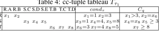
Example 3.5 Tab. 4 shows the tableau associated with the cc-tuple τ1=(Id1Id5Id8). The condition sets condτ and Cq are displayed in two different columns.

Let us now illustrate how Tτis used to identify picky conditions in the query q (elements of Cq) that are considered responsible for pruning the cc-tuple τ from the query result.

Example 3.6 First, we focus on τ1and on the two columns condτand Cqof Tab. 4. The condition x1=1 in condτcontradicts the condition x1>3of Cq. This leads us to conclude that x1>3is a picky condition. The conditions involving x2in condτ and Cqare simultaneously satisfied, as x2=3 ∧ x6=3 ∧ x2=x6is true.

Similarly, we identify the rest of the picky conditions in the column Cq and eventually obtain the set of picky conditions w.r.t. τ1that is {x1>3, x7≥8, x4=x8}. This set provides all the conditions that have to be corrected so that the cc-tuple τ1appears in the result of q. We also say that τ1is a picked cc-tuple w.r.t. the conditions {x1>3, x7≥8, x4=x8}.

Definition 3.5 (Picky conditions w.r.t. τ) With the same assumptions as before, the set of picky condi-tions w.r.t. τ is defined by P Oτ={c|c∈Cq and condτ 6|= c}.

Table 4: cc-tuple tableau Tτ1

R.A R.B S.C S.D S.E T.B T.C T.D condτ Cq

R x1 x2 x1=1 x2=3 x1>3, x2=x6

S x3 x4 x5 x3=1 x4=4, x5=8 x4=x8x5≥ 3

T x6 x7 x8 x6=3 x7=4 x8=5 x7≥ 8

Notation 3.1 (Picked and passing cc-tuple τ w.r.t. op) A cc-tuple τ is picked w.r.t. a condition c iff c∈P Oτ. Otherwise, τ is said to be a passing cc-tuple.

The Why-Not answer includes an explanation for each cc-tuple τ∈CCT (tc, I)and takes the form of

a polynomial over conditions occuring in the query.

Definition 3.6 (Why-Not answer) With the previous assumptions, the Why-Not answer is defined as T WNA(q, tc, I) = X τ∈CCT (tc,I) Y c∈P Oτ c

Example 3.7 For the purpose of the presentation, we need to name each condition of Cqfor our running

example as follows:

name op2 op3 op4 op5 op6

condition x1>3 x2=x6 x7≥8 x4=x8 x5≥3

In Ex. 3.6, we found that {op2, op4, op5}are the picky conditions for τ1, which leads to the term op2∗ op4∗ op5. Given the 12 cc-tuples of our example, we obtain the following polynomial: 2 ∗ op2∗ op5+ 2 ∗ op2∗ op4∗ op5+ 4 ∗ op2∗ op3∗ op5+ 2 ∗ op2∗ op3∗ op4+ 2 ∗ op2∗ op3∗ op4∗ op5. In the polynomial, each addend, composed by a coefficient and a condition combination, captures a way to obtain the missing answers. For instance, the combination op2∗ op3∗ op5indicates that if op2and op3and op5are correctly repaired, the missing answer will be produced by the query q. Then, the sum of its coefficient 4 and the coefficient 2 of its sub-combination op2∗ op5indicates that we will get at most 6 instances of the missing answer by repairing this combination.

We justify modeling each P Oτ with a product by the fact that in order for τ to ‘survive’ up to the query result, every single picky condition w.r.t. τ must be ‘repaired’. The sum of the products of each τ ∈CCT (tc, I)stems from the fact that, if any addend is ‘correctly repaired’, the associated τ will return the missing answer.

The coefficients of the polynomial provide the means to estimate the cardinality of the instances of the missing answers that will be obtained, when a combination x is repaired. More precisely, the sum of the coefficients of all sub-combinations of x provides an upper bound on the number of missing answer instances that could be recovered.

3.5 Why-Not Answer Properties

In this section, we compare the notion of Why-Not answer introduced in this paper (next called TED Why-Not answer) with the NedExplain Why-Not answer [5]. First, we show that the TED Why-Not answer is robust for a large class of trees. Then we show that for simple Why-Not question s, TED subsumes NedExplain.

Robustness of TED Why-Not answer. NedExplain Why-Not answers are defined for query trees, so we have to explain how TED Why-Not answers are defined for query trees. To this end, we associate a tableau query to a query tree in the obvious manner. To simplify the discussion, we assume that query

trees are built using (i) relation schemas as leaf nodes and (ii) cartesian product" and selection σcwhere cis a condition as internal nodes. W.l.o.g., we do not consider projection here.

Intuitively, in order to build a query tableau q from a query tree T , one associates a row to each leaf

node and then rewrites the condition using the function hAtt. Then, the TED Why-Not answer for the

query tree T is defined as the TED Why-Not answer for q. Thus, of course, two query trees sharing the same tableau representation have the same TED Why-Not answer.

Now, let us explore the other direction in order to characterize the set of query trees equivalent w.r.t. the TED Why-Not answer. We start by associating a class of query trees to a query tableau q.

Definition 3.7 (Query trees w.r.t. q) Let q=(_, Tq, Cq)be a query tableau and assume that |Sq|=n. The set opSet of tree operators associated with q is the set of selections {σ_h−1

Att(c)|c∈Cq}.

A query tree T is associated with q iff (i) it has exactly n − 1 cross product nodes, (ii) it has exactly one node for each selection in opSet, (iii) it has exactly one leaf node for each relation R in Sq, and finally, (iv) it is equivalent to q.

Intuitively, the difference between two trees T1and T2associated to the same query q is the order of the operators in the trees.

Theorem 3.1 Given a query q, TED Why-Not answer is unique up to isomorphism for all possible query trees associated to q.

The above theorem states that two equivalent query trees obtained by some reordering of their op-erators lead to the same Why-Not answer. Clearly, this behavior is more robust than the behavior of NedExplain, where the Why-Not answer may differ for every equivalent query tree.

The question about other (equivalent) query trees sharing the same Why-Not answer property remains open although we have investigated several directions. We have considered minimization of the tableau leading to equivalent query trees. We also have considered saturating the query conditions, once again leading to equivalent query trees. However, these query trees do not produce the same Why-Not answer as counterexamples show.

Subsumption of NedExplain result by TED Why-Not answer. The next result shows that the TED Why-Not answer subsumes the NedExplain Why-Not answer.

Theorem 3.2 Let q be query tableau over the shema Sqand I be an instance over Sq. Let tcbe a simple Why-Not question. Assume that T is a query tree representation of q. Let

N ED={T0|T0is a subtree in T } be the NED Why-Not answer w.r.t. T , I and tc, and let

T ED={x|xis a combination in T W NA(q, tc, I)}

be the TED Why-Not answer w.r.t. q, I and tc. Then, we have that

∀T0∈N ED ∃x∈T ED s.t. c∈x

where c is the condition of the rooting operator of the subtree T0_.

4 Naive Ted Algorithm

This section summarizes the Ted algorithm that naively computes the Why-Not answer polynomial by implementing in a straightforward manner what we discussed in Sec. 3. Further details are available in [4].

Briefly, Ted firstly computes all the cc-tuples w.r.t. the Why-Not question and then for each cc-tuple, it identifies the picky query conditions, constructing along the way the Why-Not answer polynomial. It is easy to see that such a straightforward implementation is computationally prohibitive, as it implies computing and enumerating the set of cc-tuples CCT (tc, I)(Def. 3.3).

In principle, CCT (tc, I)can be computed by executing an SQL statement with the conditions of tc over I. This is however a costly query, as it requires in most cases performing cross products of subsets of the input instance relations. To counter this problem, we introduce the valid partitioning of Ttc that

first computes sets of partial cc-tuples efficiently, which then need to be combined.

Definition 4.1 (Valid Partitioning of Ttc). The partitioning of Tq into k partitions P art1, . . . , P artk,

denoted P artitioning = {P arti, . . . , P artk}, is valid for Ttcif each P artiis minimal w.r.t. the

follow-ing property:

if R∈P arti and R0∈Sq s.t. ∃c∈Cq with hAtt(var(c))∩Att(R)6=∅and hAtt(var(c))∩Att(R)6=∅then

R0∈P arti.

A tuple τ∈CCT (tc|P arti, I|P arti)is called a partial cc-tuple.

Example 4.1 In our example, the valid partitioning (see Tab. 3) is P art1={R, S}(because of the con-dition x2=x4, where x2, resp. x4 refers to R.B, resp. S.D) and P art2={T }. Examples of partial cc-tuples include Id1Id5∈CCT (tc|P art1, I)and Id8∈CCT (Ttc|P art2, I).

It is easy to prove that the valid partitioning of Ttcis unique and the following lemma states how to

compute CCT (tc, I)based on partial cc-tuples.

Lemma 4.1 Let P={P art1, . . . , P artk}be the valid partitioning of Ttcand I database instance over

Sq. Then,

CCT (tc, I)= " P arti∈P

CCT (t_{c|P arti}, I_{|P arti}).

Although this partitioning helps to reduce the computation and materialization of cross products, Ted’s worst case time complexity remains O(n|Sq|₎, n=max({|I

R| |R∈SQ). So, as validated also by experiments in Sec. 6, Ted is not of practical interest.

5 Efficient Ted++ Algorithm

The main feature of Ted++ is to completely avoid cross product materialization, thus significantly re-ducing both space and time consumption. To achieve this, Ted++ performs two main paradigm shifts. First, instead of tracing picked cc-tuples, it focuses on tracing passing cc-tuples. Second, Ted++ starts with a “polynomial template” that includes all possible condition combinations (addends) with variable coefficients to then incrementally and mathematically compute the coefficients for these addends.

Alg. 1 presents the main steps of Ted++. Ted++’s input includes the query q=(Tq, Cq), the Why-Not question tc and the input database instance I. The following subsections discuss the individual steps of the algorithm in more detail.

5.1 Preprocessing

The first step of Ted++ (Alg. 1, line 1) is the computation of the “polynomial template” mentioned above, which is simply obtained by computing the power set of the query condition set Cq, from which the empty set is discarded.

Example 5.1 For our example (Fig. 3), the search space is {op2, op3, . . . , op2op3, . . . , op2op3op4op5op6}; its size is 25_{− 1.}

Algorithm 1: Ted++

Input: query q, instance I, Why-Not question tc

Output: W NAP oly, the Why-Not answer polynomial

1 Initialization of CombSet, and Ttc %preprocessing 2 P artition←findValidPartitioning(Ttc); (Def. 4.1) 3 for P art in P artition do

4 DB← Materialize VP art% based on T_{tc|P art}; 5 CombSet←PickyCombinations(CombSet, DB);

6 W N AP oly←ExactAnswer(CombSet); %postprocessing

7 return W NAP oly;

All along the algorithm, Ted++ maintains a data structure called CombSet. For each condition com-bination x it registers a tuple combx=(opSet, partS, V, #P ick)where opSet contains the conditions in x, partS is a set of partitions (defined later on), V is a view definition meant to store the passing partial cc-tuples w.r.t. x. Finally, #P ick is the number of picked cc-tuples w.r.t. x and all its super combina-tions (i.e., combinacombina-tions containing x). To simplify the discussion, we refer to #P ickxas the number of picked cc-tuples w.r.t. x. The ‘exact number’ of picked cc-tuples w.r.t. x is computed in a postprocessing step (Alg. 1, line 6).

As in Ted, the second preprocessing step builds the conditional tableau Ttcas describe in Sec. 3.3.

5.2 Partial CC-Tuples Computation

To compute the partial cc-tuples, the tableau Ttcis first partitioned according to Def. 4.1 (Alg. 1, line 2).

Each partition P art is associated with a view VP art, called partition view. VP artis defined as the query corresponding to the tableau Ttc|P art(see example below) and is materialized in the database (line 4).

Example 5.2 We are given P art1={R, S}and P art2={T }(see Ex. 4.1). The view definition VP art1

relies on the partial tableau Ttc|P art1except for the outmost projection. The projected attributes are those

constrained by the query q, plus the relation Ids in P art1, that is {R.A, R.B, S.D, S.E, R_Id, S_Id}. Similarly for P art2, the set of projected attributes is {T.C, T.D, T.T _Id}. This results in the query definitions given below and the materializations shown at the bottom of Fig. 4.

VP art1 VP art2

SELECT R_Id, S_Id, R.A,R.B,S.D,S.E FROM R, S WHERE R.B < S.D SELECT T_Id,T.B,T.C,T.D FROM T WHERE T.C ≤ 9

5.3 Picky Condition Combinations

The next step (line 5) of Alg. 1 identifies picky condition combinations. The pseudo-code of the function

P ickyCombinationsis given in Alg. 2.

First, the set of condition combinations CombSet is traversed in ascending order of condition combi-nation size (i.e., from size 1 to |Cq|, see Alg. 2, line 1). For each combination x we compute the number of picked cc-tuples #P ickx, using in each iteration results obtained in previous ones. To calculate #P ickx we rely on the calculation of the number of picked partial cc-tuples |P P ickx|. To do that, we rely on the set of partitions partSxin combx.

Let x be an atomic combination, i.e., one condition op. When op is simple, it refers exactly to one relation R, which belongs to one partition P art hence partSop={P art}. When op is complex, it refers to two relations R and S and either both relations belong to the same partition P art and partSop={P art} or they belong to different partitions P art1and P art2and partSop={P art1, P art2}. Recall that, each partition P art is associated with a partition view VP artthat stores the partial cc-tuples over P art. We

Algorithm 2: PickyCombinations Input: CombSet, DB

Output: CombSet

1 for k=1 to |Cq| do

2 for combx∈CombSet s.t. |opSetx|=k do 3 Compute partSx;

4 if k=1 then

5 DB←Materialize Vx; (Def. 5.1) 6 else

7 if Vxneeds to be materializedthen

8 (combx1,combx2) ← SelectSubCombinations(Vx);

9 if Target schemas of V_x1and V_x2share common attributes Attthen 10 Vx← V_x11AttV_x2;

11 DB←Materialize Vx;

12 else

13 | Vx|←multiply sizes of sub-combination views in x; 14 |P P ickx| ←Apply Equ. (G);

15 #P ickx←Apply Equ. (A); 16 return CombSet;

associate with P artSopthe set of partition views V={VP art|P art∈P artSop}. We now generalize to a non atomic condition combination x where opSetx⊆Cqand define partSx= ∪op∈opSetxpartSop.

Example 5.3 Consider the two atomic combinations op2(x1>3)and op3(x2=x6). Looking at Tab. 3, we see that op2refers only to P art1, whereas the variables of op3span over P art1and P art2. Hence, partSop2={P art1}and partSop3={P art1, P art2}. Considering the condition combination x where

opSetx={op2op3}, we obtain P artx={P art1, P art2}. Fig. 4 associates to all atomic combinations their respective sets P artopusing edges between op and partition views.

Using partSx, the number of picked cc-tuples w.r.t. combination x, i.e., #P ickxis computed by

Equ. (A):

#P ickx= |P P ickx| × Y

P art∈partSx

|VP art|, _(A)

where partSx=P artitioning \ partSx. Note that when partSx is empty, we abusively consider that

Q

∅=1. Intuitively, the above formula extends the partial cc-tuples to “full” cc-tuples over all partition schemas.

The presentation now focuses on calculating #P ickx, by firstly calculating |P P ickx|. Two cases arise depending on the size of the condition combination.

Atomic condition combinations. We start with considering condition combinations x s.t. |opSetx|=1

(Algorithm 2, Line 5). To find the number P P ickxof picked partial cc-tuples w.r.t. x we compute and materialize the set of passing partial cc-tuples through the query provided below:

Definition 5.1 (Condition View.) Let op be a condition, partS its associated set of partitions and V its associated set of partition views. Then, the condition view Vopfor op is specified by:

Vop=     

π_{{Rid|R∈P art}}(σop[VP art])if partS={P art} π_{{Rid|R∈P art1∪P art2}}([VP art1]1op[VP art2])

if partS={P art1, P art2} Example 5.4 Given P artSop3={P art1, P art2}, Vop3is

Fig. 4 shows the materialization of all operator views. Note that the materialization of view V2is empty, hence, no associated materialization is presented.

We can now compute the number of picked partial cc-tuples for an operator op by: |P P ickop| =

Y

P art∈partSop

|VP art| − |Vop| (B)

Example 5.5 For op3, we have |Vop3|=4. So, |P P ickop3|=|VP art1|×|VP art2|−|V3|=3×4−4=8. Since

all partitions of P artitioning are in partSop3, applying Equ. (A) results in #P ickop3=P P ickop3=8.

Opposed to that, for op4, |P P ickop4|=|VP art2|−Vop4=4−2=2, so #P ickop4=2 ∗ 3 = 6. The results of

Equ. (A) and (B) are shown in Fig. 4 for all remaining atomic combinations.

Non atomic condition combinations. After processing all atomic conditions, we proceed with non-atomic ones (Alg. 2, lines 6-13).

Let opSetx={opi|i=1 . . . N }be the set of conditions of the combination x. Intuitively, to find the picked partial cc-tuples w.r.t. x, we need to find the picked partial cc-tuples common to op1 and . . . and opN. These common cc-tuples are in the intersection of the sets of picked partial cc-tuples of op1 . . . opN, stored in the materialization of Vop1. . . VopN. As we will see, in order to compute the intersection

(or simply get its cardinality), we may have to use, in addition to the condition views Vopi, all views

associated with the sub-combinations of x, including x itself.

To describe this most complicated step of the algorithm, we start by developing a simplified case.

Assume that all condition views have the same target schema Attx={R_Id|R∈P and P ∈partSx}.

The set of picked partial cc-tuples w.r.t. x is computed as the intersection of the complements of the condition views storing the passing partial cc-tuples:

P P ickx= Vop1∩ · · · ∩ VopN = Vop1∪ · · · ∪ VopN (C)

As our design decision was to only materialize passing partial cc-tuples of views Vi, we rewrite P P ickx as: P P ickx= πAttx[ " P art∈partSx VP art] \ [ op∈opSetx Vop _(D)

Given the assumption that all condition views have the same schema, applying the set operators (difference, union) is well defined, and so is the query P P ickx. However, in the general case, this assumption does not hold. Thus, to deal with the general case, the previous equations need to be rewritten by “extending” condition views Vopto views Vopextover a common schema with attributes Attx(as defined above):

V_opext= πAttx\Attop[ "

P art∈partSx\partSop

VP art] × Vop (E)

This extended view substitutes Vopin Equ. (D) in the general case and we thus obtain the following query to compute P P ickx: P P ickx= πAttx[ " P art∈partSx VP art] \ [ op∈opSetx V_opext _(F)

As already said, the main feature of Ted++ is to avoid computing cross products, so clearly, we do not want to compute the cross product introduced in Equ. (E) and (F). Fortunately, remember that we are