Lower and upper bounds for deterministic convergecast with labeling schemes

(1)

HAL Id: hal-02650472

https://hal.archives-ouvertes.fr/hal-02650472v2

Submitted on 10 Aug 2020

HAL is a multi-disciplinary open access

archive for the deposit and dissemination of

sci-entific research documents, whether they are

pub-lished or not. The documents may come from

teaching and research institutions in France or

abroad, or from public or private research centers.

L’archive ouverte pluridisciplinaire HAL, est

destinée au dépôt et à la diffusion de documents

scientifiques de niveau recherche, publiés ou non,

émanant des établissements d’enseignement et de

recherche français ou étrangers, des laboratoires

publics ou privés.

with labeling schemes

Gewu Bu, Zvi Lotker, Maria Potop-Butucaru, Mikael Rabie

To cite this version:

Gewu Bu, Zvi Lotker, Maria Potop-Butucaru, Mikael Rabie. Lower and upper bounds for deterministic

convergecast with labeling schemes. [Research Report] Sorbonne Université. 2020. �hal-02650472v2�

(2)

convergecast with labeling schemes

Gewu Bu

Sorbonne University LIP6, France [email protected]

Zvi Lotker

Bar Ilan University, Ramat-Gan, Israel, Ben Gurion University, Israel

Maria Potop-Butucaru

Mikaël Rabie

Abstract

In wireless networks, broadcast and convergecast are the two most used communication primitives. Broadcast instructs a specific sink (or root) node to send a message to each node in the network. Convergecast instructs each node in the network to send a message to the sink. Without labels, deterministic convergecast is impossible even in a three-nodes network. Therefore, networking solutions for convergecast are based on probabilistic approaches or use underlying probabilistic medium access protocols such as CSMA/CA or CSMA/CD. In this paper, we focus on deterministic convergecast algorithms enhanced with labeling schemes. We investigate two communication modes:

half-duplex (nodes either transmit or receive but not both at the same time) and full-duplex (nodes

can transmit and receive data at the same time). For these two modes we investigate time and labeling lower and upper bounds. Even though broadcast and convergecast are similar, we prove that, contrary to broadcast, deterministic convergecast cannot be solved with short labels for some topologies. That is, O(log(n)) bits are necessary to solve deterministically convergecast where n is the number of nodes in the network. We also prove that O(n) communication time slots is required. We provide solutions that are optimal in the worst case scenarios, in terms of labeling and communication.

2012 ACM Subject Classification General and reference → General literature; General and reference

Keywords and phrases Dummy keyword

Digital Object Identifier 10.4230/LIPIcs...23

Acknowledgements I want to thank . . .

1 Introduction

Convergecast and Broadcast are basic communication primitives in wireless networks. In Broadcast, one source node needs to send its message to all the other nodes in the network.

We say that the broadcast succeeded if at the end of the broadcast, all the non-source nodes in the network received successfully at least once the target message sent by the source node. On the other hand, for the convergecast, each node in the network has its own message that needs to be sent to one special node, called Sink. The convergecast is a success if at the end of the process, the sink node received successfully all the messages sent from all the other nodes in the network. The convergecase strategies are widely used in sensor networks for collecting critical data from a target area. In many applications, nodes that need to communicate with the sink might not be able to maintain a direct connection with it. Therefore, in many

licensed under Creative Commons License CC-BY Leibniz International Proceedings in Informatics

(3)

situations the communication with the sink has to be multi-hop. Our research focuses on the deterministic distributed convergecast in the multi-hop topologies. The purpose of the algorithm is to coordinate and to schedule when and how nodes send and forward messages in the network to finally achieve efficiently the convergecast. More precisely, we are interested in multi-hop wireless networks subject to collisions. In practice, the overlapping among wireless signals sent simultaneously into the same wireless channel might occur during the transmission. The overlapping signals are difficult to be distinguished at the receiver node if these overlapping signals use the same carrier frequency. We call this situation collision. Note that, in reality, even if the receiver experienced a collision during the signal decoding, the receiver still has a chance to recover correctly the interfered target signal among all the interference signals. This chance strongly depends on the reception strength and modulation mode of receiving signal, which are hard parameters to be ensured. If a message sent by a node entered in collision with other transmissions, without additional re-transmission mechanism, the message will be permanently lost. It follows that the convergecast process failed. An efficient deterministic convergecast algorithm therefore should completely avoid any collision instead of letting receiver nodes try again their luck.

The convergecast problem takes its roots in the practical sensor networks area. One of the first to investigate the problem from both theoretical and practical aspects, [4], consider the setting where each sensor node in the network has a single message to be sent to the sink. The authors target to find the optimal (minimal) time rounds scheduling to achieve the gathering of all the messages at the sink. The problem is referred as minimum information

gathering time problem. In [4] the authors prove that even in centralized settings this problem

is NP-Complete on general topologies. In [4] and [20] the authors propose similar centralized convergecast algorithms that finish in at most 3n − 3 rounds, where n is the number of nodes. The proposed solutions work only for line and tree topology networks. Distributed convergecast algorithms are proposed in [10] and [11]. The proposed algorithms archive the theoretic lower bound for line and tree typologies: max(3nk− 3, n) rounds, where nk

is the number of nodes in the longest branch of the tree. For general graphs the proposed algorithms needed at most 3n − 2 rounds. However, the price of decentralization is important in this solution. Nodes need to store their IDs, the ID of the branch they belong to and the number of nodes in this branch. Moreover, to avoid collisions, a collision resolution mechanism is proposed: by passing an additional information exchanging phase among nodes, each node needs to store a n × n collision table. Instead of requiring additional exchanging phase to create and store the collision table, our proposition needs only O(log(n)) bits of additional information to achieve the convergecast.

On another line of research, multi-channel-based convergecast was investigated in [16], [18] and [19]. By using different communication channel/frequency, a receiver node can successfully receive up to k message simultaneously, where k is the number of usable channels. The best to date results in multi-channel settings is only for line networks: the lower bound of convergecast is 2n − 1 by using dn/2e channels. In this work we are interested in general network topologies and single channel transmissions.

Similar to the minimum information gathering time problem, the minimum data

aggrega-tion time problem is investigated in [17] and [21]. In data aggregaaggrega-tion problem nodes can

aggregate multiple received messages into a new message and send only the new message instead of old ones to reduce the chance of collisions. In [17] the authors propose the best to date centralized algorithm that takes at most 12R + δ − 11 rounds, where R is the radius of the network and δ is the maximum degree of the network. In [21] the authors proposed distributed algorithms that take at most 2n rounds for line networks, 3n + k rounds for

(4)

general networks with n nodes and k branches. However the solution proposed in [21] needs an additional collision avoidance mechanism similar to the one proposed in [11].

In the current work we investigate the gathering of information (convergecast) without aggregation in multi-hop general networks where each node is enhanced with labels. Labels are additional information used in order to avoid collisions. Each node is enhanced with a pre-computed label that instructs it when to send/receive or sleep.

Labeling is an interesting mechanism that was used for decades in distributed algorithms

to reduce the computational complexity. The basic idea of labeling is to allocate labels (i.e. pieces of information computed offline) to the nodes of a network in order to advise nodes in taking some decisions. Via the pre-allocated labels nodes can be assigned to specific behaviors during the online execution of the distributed algorithm. Labeling schemes proved themselves as an efficient mechanism to improve algorithms efficiency and even bypass impossibility results. Labeling schemes have been designed in [1], [12] and [15] to compute network size, the father-son relationship and the geographic distance between nodes in the network, respectively. It has been also used in [9], [13] and [14] in order to improve the efficiency of Minimum Spanning Tree, Leader Election and Topology Recognition algorithms, respectively. Furthermore, [5] and [8] exploit labeling to improve the existing solutions for network exploration by a robot/agent moving in the network. Generally speaking, the utilisation of labels implies to use additional memory space to store allocated labels in each node.

Interestingly, only [2] and [7] designed deterministic distributed broadcast primitives enhanced with constant labels for multi-hop wireless networks subject to collisions. Labels are used in both works as a scheduling mechanism in order to avoid collisions. In the current work, we are interested in the information gathering (covergecast) problem in collision-present communication environment. Although [6] investigated the covergecast problem in tree topology, the present of collision during the communication has never been addressed in these settings. Compared with broadcast, convergecast is more challenging: in broadcast, only one source node starts the transmission and the other nodes receive and forward it. Convergecast instructs all non-sink nodes to transmit their messages to a specific node called

sink. The convergecast has a higher number of transmissions to schedule and therefore a

higher number of potential collisions may occur during the algorithm execution.

1.1 Our contributions

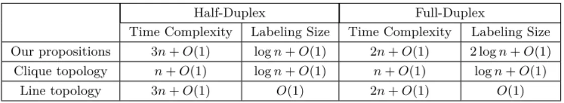
We address for the first time the deterministic convergecast problem with labeling schemes in arbitrary networks subject to collisions. We propose lower and upper bounds in terms of time and labeling complexity for two communication models: half-duplex (nodes cannot send and receive simultaneously) and full-duplex (nodes send and receive simultaneously). First, we prove that in arbitrary networks, O(n) rounds are necessary to deterministically solve convergecast and at least log(n) + O(1) bits are needed. Furthermore, we propose a deterministic convergecast algorithm for a network of n nodes in half-duplex model that needs 3n + O(1) rounds and uses labels of size log(n) + O(1) bits. In the case of full-duplex we propose a deterministic convergecast algorithm that needs 2n + O(1) rounds and labels of size 2log(n) + O(1) bits. Our results are summarized in Table 1.

2 System model

We represent the network by a connected graph G(V, E), where V is the set of all nodes in

(5)

Table 1 Lower and upper bounds for deterministic convergecast with labeling

Half-Duplex Full-Duplex

Time Complexity Labeling Size Time Complexity Labeling Size Our propositions 3n + O(1) log n + O(1) 2n + O(1) 2 log n + O(1) Clique topology n + O(1) log n + O(1) n + O(1) log n + O(1)

Line topology 3n + O(1) O(1) 2n + O(1) O(1)

G. For any node v ∈ V , if e(u, v) ∈ E, we say that node v is in the communication range

of node u. We consider wireless transmissions. That is, when a node sends a message, this message will be transmitted as a wireless signal into a shared wireless channel, all nodes within the wireless communication range (i.e. graph neighbors) of the sender can receive this transmission.

We consider a distinguished node in the network sink. The convergecast consists in allowing each node in the network to transmit a message to the sink. Each node has a First

In First Out (FIFO) message buffer initially containing only the message the node wants to

transmit to the sink. Note that the sink has no message initially in its buffer.

We consider that nodes have synchronized clocks and time is divided in slots. Nodes may use two communication modes: Half-duplex (sending and receiving messages cannot be done simultaneously) and Full-duplex (nodes are allowed to send and receive in the same time). Appendix A.1 shows the comparison between half-duplex and full-duplex modes.

In the Half-duplex mode in each time slot each node can be in one of the following three different states: 1) Listen 2) Send and 3) Sleep. A node in state Sleep, turns itself off temporary (i.e. it does not listen to the channel neither send any message). Nodes in state

Send will take out the first message from their buffer (if there is any) and send this message

to the wireless channel, to all its neighbors. A node in state Listen will listen to the channel and wait for incoming messages..

In the Full-duplex mode, in each time slot, nodes can be in one of the states 1) Listen 2)

Send, 3) S&L 4) Sleep. State S&L represents a node that can both transmit and receive at

this time slot.

A node can only be in one state during a time slot and it may change its state in the next time slot. Note that we assume that nodes need a whole time slot for sending or receiving completely one message. We also assume that the message propagation time is negligible. That means, if a node v in state Send sends a message at the beginning of a time slot, its neighbours in state Listen will receive the message at the end of the time slot.

To receive a message successfully in a time slot, a node needs to be in state Listen or

S&L and that exactly one of its neighbors send a message (meaning having a non-empty

buffer and be in state Send or S&L). If multiple neighbors are sending simultaneously a message in that time slot, a conflict occurs, and no message is received (and the content of the messages sent might be lost forever, if no more nodes have it in their buffer).

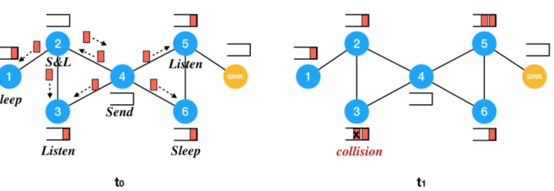
Figure 1 shows an example of the transmission process.

In the context of convergecast, the sink node should receive in a finite bounded time all the messages sent by every other node. We propose two labeling based convergecase algorithms for half-duplex and full-duplex communication modes. Using per-computed additional information offline, the labels, each node therefore extrapolates at what time it should wake up, send and receive message without creating collisions during the online execution. In the following sections, we present our solutions and lower bounds for the two communication modes.

(6)

Figure 1 Initially, each non-sink node has a message in its buffer. At time t0, nodes are in different states: node 4 in Send, node 2 in S&L, nodes 3 and 5 in Listen and nodes 1 and 6 in

Sleep. Nodes 4 and 6 begin to send their messages by taking them out from their buffers and send

the message to all nodes in its transmission range. At time t1, nodes 2 and 5 receive the message

from node 4. Node 1 and 6 are sleeping, they therefore don’t receive any message. However two messages from node 2 and node 4 arrive at node 3 simultaneously. A collision occurs therefore at the node 3.

We want to work with the minimal hypothesis on the nodes of the graph, to allow to have an algorithm that would also work in stronger variants. Hence, we suppose that the nodes are anonymous, and that there is no node numbering. A node is only aware if it is or not the sink node.

For the pre-processing of the labels, we use a centralized algorithm. That one can give temporary identifiers to the nodes for its own computation. However, the identifiers will not stay on the nodes afterward, unless they are included in the labels provided by the algorithm.

3 Lower Bounds

ILemma 1. Any deterministic algorithm that solves the convergecast problem on a path

takes at least 3n−6 time slots in the Half-duplex Model and 2n−4 time slots in the Full-duplex Model.

Proof. Consider the network where nodes form a path rt= u1, u2, . . . , un. We know that,

∀i > 1, the node ui needs to transmit the information of the nodes ui, ui+1. . . un, as the

topology is a path. As a node can only transmit one message in a time slot, the node ui will

need N − i + 1 time slots to transmit its information and the information of the nodes after itself in the path. When a node ui successfully transmits information to ui−1, node ui−1

must be listening, meaning that node ui−2cannot transmit during that period (otherwise,

there would be a conflict in ui−1).

Hence, when node u4 transmits n − 3 times, node u2 cannot perform any of its n − 1

necessary transmissions. As those 2n − 4 communications need to happen, and none can happen at the same time, we get the second lower bound. If nodes cannot transmit and receive at the same time, node u3 transmits n − 2 times, listens n − 3 times. Moreover, it

must sleep when node u2successfully transmits n − 1 times, as it cannot transmit to u2(as u2

is already transmitting and cannot be listening) and cannot receive from u4 (as there would

be collisions as both u2 and u4 are neighbors to u2). This gives the first lower bound. J ILemma 2. Any deterministic algorithm that solves the convergecast problem on a clique

(7)

Proof. Consider a clique network where all nodes except the sink cannot be differentiated. After getting labels, two non-sink nodes can be differentiated if and only if they have two different labels.

Let’s suppose we have two nodes with the same label. Each time they Listen during the same time slot, if a single message comes (i.e. there is no interference), it is the same message, as it means that a single node of the clique is transmitting. Hence, no symmetry can be broken between those two nodes, as they have the same starting state and their history of received information will be the same. Therefore, they will always Transmit at the same time. When it happens, no node can get their message, as they are connected to those two nodes, and the messages will collide. By contradiction, it means that each label of the non-sink nodes must be unique.

We need n − 1 different labels for each non-sink node to be able to perform a convergecast on a clique. With log(n − 1) − 1 bits, we can make 2log(n−1)−1_{≤ n − 2. Hence, we need at}

least log(n − 1) ≥ log n − 1 bits. _J

IRemark 3. In this lemma, the absence of identifiers is crucial, as unique identifiers means that each pair of nodes can be differentiated. In the particular case of the clique with unique identifiers, there is a solution for the convergecast without labels: the sink node listens in each time slots, and a non-sink node with identifier k transmits its own information in the time slot k. The convergecast will finish in K time slots, where K is the maximal identifier given to a node in the clique.

ITheorem 4. There exists a graph topology in which the convergecast needs 3n + O(1) time

slots in the half-duplex mode and 3n + O(1) time slots in the full-duplex mode. Moreover, the labels must be of size log n + O(1).

Proof. The sink node rt is connected to a path of length four rt− u1− u2− u3− u4. The

node u4 is connected to a clique of size n − 5. With a similar proof that in Lemma 1, we

know that u2 will need 3n + O(1) time slots in the half-duplex mode and 2n + O(1) time

slots in the full-duplex-mode to receive and transmit the information of u3 and the nodes in

the clique. Moreover, in the clique, by following the same proof of Lemma 2, we know that log(n − 5) − 1 bits are needed for the labels. _J

4 Convergecast in Half-duplex Mode

4.1 Labels for Half-duplex communication mode

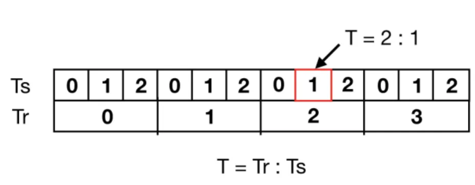
We recall that in the half-duplex communication mode nodes cannot transmit and receive in the same time slot. To ease the reading of our algorithm, we consider that time is divided in rounds and each round is divided in three time slots (numbered from 0 to 2). We represent the time T as T =< Tr: Ts > where Tr represents the current round and Ts the current

slot in the round Tr. For example, time T =< 2 : 0 > represents time slot 0 of round 2 (see

Appendix A.2). Basically, time T =< Tr: Ts> corresponds to the time slot 3Tr+ Ts.

For the convergecast in half-duplex mode, each node v ∈ V starts in state Sleep and gets a pre-computed label in format < yv: hv > at the beginning of the convergecast algorithm.

The first part of the label, y ∈ N, represents the round indicator when v has to wake up. The second part of label, h ∈ {0, 1, 2}, guides the actions (i.e. Listen, Send or Sleep) that v should take when it wakes up. In the next section, we describe the actions each node takes at each time based on its label, then we describe in Section 4.3 the labels allocation scheme for the half-duplex mode.

(8)

4.2 Convergecast Algorithm for Half-Duplex

Algorithm 1 indicates the actions a node should take at a specific time T =< Tr: Ts> based

on its label < y : h >. An execution example of Algorithm 1 can be found in Appendix B.

Algorithm 1 Convergecast algorithm executed by node v with label < yv: hv> at time T =< Tr: Ts>

if Tr≥ yv then

if Ts== hv mod 3 then

node v turns in state Send.

else if Ts== (hv+ 1) mod 3 then

node v turns in state Sleep.

else if Ts== (hv+ 2) mod 3 then

node v turns in state Listen.

4.3 Labels Allocation for Half-duplex mode

This section is dedicated to the labels computation scheme for half-duplex mode. The label

< yv : hv > of node v has two parts: yv and hv. These two parts of the label will be

computed by Algorithms 3 and 4, respectively. The first part of the label, y, is computed by Algorithm 4 that performs a Depth-First-Search (DFS) exploration of nodes starting with the sink node. Algorithm 3 computes for each node the second part of the label, h, based on the shortest path distance of each node to the sink. Algorithm 2 computes these distances using a Breadth-First-Search (BFS) strategy and outputs a vector D which records for each node its distance to the sink.

Algorithm 2 BFS-distance algorithm

%Given a connected graph G(V, E) with rtas the sink node.

%For all v ∈ V , N (v) is the set of v’s neighbors.

%Let Vs, Vv be two empty node sets; a vector D[|V |] = ∅ to record the shortest

%distance of each node to rt; d = 0; S is a LIF O stack initially empty.

PUSH rtinto S. Vv← {rt} D[rt] ← d

while S 6= ∅ do

POP all nodes from S.

Vs← {all popped nodes}.

d ← d + 1

for each node k ∈ V \ Vs such as ∃j ∈ Vs: k ∈ N (j) do

PUSH k into S.

Vv← Vv∪ {k}. D[k] ← d

return D

4.4 Correctness of Convergecast for Half-duplex mode

Now we prove the correctness of Algorithm 1. Firstly, we introduce some notations and definitions.

(9)

Algorithm 3 h allocation for Half-duplex mode

%Let H be a vector H[|V |] to record the second label < − : hv>

%of each node v.

Compute D[n] with Algorithm 2.

for Each node v ∈ V do

Node v gets its hv label: H[v] ← 2 − D[i] mod 3

Algorithm 4 y allocation algorithm for Half-duplex

%Let Y be a vector Y [|V |] to record the first label < yv: − >

%of each node v.

%Table D[n] contains the distance of each node in V to rt.

%Let Vv, Vs be two empty sets; CP OP = 0, CLP OP = 0 initially;

%an index x = rtinitially; S is a LIF O stack initially empty.

PUSH rtinto S. Y [rt] ← 0

Vv← {rt}

POP one node v from S.

Y [v] ← CLP OP − D[x]

CP OP ← CP OP + 1 Vs← Vs∪ {v}

if N (v) \ Vv6= ∅ then

PUSH each node from N (v) \ Vv into S Vv← Vv∪ N (v)

else%Nothing to PUSH, we note as a PUSH-NULL

CLP OP ← CP OP

x ← q, where q is the next node in S is going to be popped. Vs← ∅

IDefinition 5 (Level). The level of a node v, noted L(v), is the shortest distance from v to

the sink node. L(v) equals D[v] (output of Algorithm 2).

IDefinition 6 (Round). The round of a node v is noted y(v), or yv. y(v) equals Y [v] (output of Algorithm 4).

IDefinition 7 (Neighbors). The neighbors of a node v, noted N (v), is the set of nodes u

such as e(u, v) ∈ E.

I Definition 8 (Parent Nodes). The parents of a node v is the set of nodes {u ∈ V :

(L(v) − L(u) = 1) ∧ e(u, v) ∈ E}.

IDefinition 9 (Direct Son Nodes). The direct sons of a node v, noted S(v), is the set of

nodes {u ∈ V : (L(u) − L(v) = 1) ∧ e(u, v) ∈ E}. It corresponds to the set of nodes that are pushed after we popped the node v in Algorithm 4.

IDefinition 10 (Indirect Son Nodes). The indirect sons of a node v, noted IS(v), is the

(10)

ISi(v) S

u∈ISi(v)

S(u), we have the existence of some iv such that, ∀i ≥ iv, ISi(v) = ISiv(v)

(this is clear as the set is increasing and bounded by |V |). We have IS(v) = ISiv(v).

IRemark 11. In Algorithm 4, when we pop a node v, we PUSH immediately the set of its Direct Sons. By direct induction, as S is a LIF O, when we pop a node v, we will PUSH exactly the set of its Indirect Sons before pushing any other nodes.

I Definition 12 (Direct Dominating Son Nodes). The direct dominating sons of a node

v, noted DDS(v), is the subset of S(v) with a bigger first part of a label than v’s, i.e.

{u ∈ S(v) : y(u) ≥ y(v)}.

IDefinition 13 (Indirect Dominating Son Nodes). The indirect dominating sons of a node

v, noted IDS(v), is the subset of IS(v) with a bigger first part of a label than v’s, i.e.

{u ∈ IS(v) : y(u) ≥ y(v)}.

IRemark 14. By construction of Algorithm 1 and the fact that the time slot of a node is given according to its distance to the source node modulo 3, we have the following direct observations:

The state of a node v will change following the cycle T → S → L → T → S → L. . . Nodes in the same level L(v) of v are in the same state that v; nodes in level L(v) − 1 are in one state before in terms of the state changing cycle; nodes in level L(v) + 1 are in one state later in terms of the state changing cycle explained above.

ILemma 15. Messages sent from a node v can only be received by the parent nodes of v.

Proof. According to Remark 14, when a node v is in state Send, nodes in S(v) are in state

Sleep; nodes in P (v) are in state Listen. Others neighbors of v who are in the same level of v are in state Send. The message sent from v can therefore only be received by nodes in

P (v). _J

IDefinition 16. The Parent of a node v, noted P (v), is the last node that was popped by

Algorithm 4 before v was pushed. We can notice that L(p) = L(v) − 1.

IDefinition 17. The set of Ancestors of a node v is the transitive closure of its parents, to

which we add v itself (i.e. v is its own ancestor). We say that u is an ancestor of v if it belongs to this set.

ILemma 18. At any point in Algorithm 4, x is an ancestor of v. Vs represents the direct path from x to v. More precisely, we have Vs= S

0≤i<|Vs|

Pi_{(v) and x = P}|Vs|−1_(v).

Proof. By contradiction, let v0 be the first node popped such that this property is false. It

means that we did not do a push-null right before, as otherwise Vs= v0. Let u be the previous

node to have been popped. We have, by the choice of v0, that Vs\ {v0} = S 0≤i<|Vs|−1

Pi_(u).

As we did not do a push-null right before, it actually means that v0 has been pushed

in the previous step (as it is the last element to have been added in the LIF O, and at least one element was added), when we were handling u. Hence, v0 is a direct son of u: u = P (v0). Moreover, the property of the Lemma was true for u, by the choice of v0. Hence, x = P|Vs|−2_{(u) = P}|Vs|−1_{(v). This leads to a contradiction.} _J

ILemma 19. In Algorithm 4, when we put the instruction setting the value for the round

(11)

Proof. The Lemma is true if we did a PUSH-NULL right before popping v.

Let suppose that we did not do a PUSH-NULL right before. The value given to y(v) only depends on when the POP of x happened. When we set y(v), Vscontains exactly the nodes

that were popped between the POP of x (included) and v (excluded). By Lemma 18, we have that x = P|Vs|−1_{(P (v)) = P}|Vs|_{(v), meaning that L(x) = L(v) − |V}

s|. (|Vs| \ {x}) ∪ {v}

represents the exact set of nodes that were popped since the last time CLP OP was set to

a value. Hence, we get that CLP OP = CP OP − |Vs|. This leads to the expected result:

y(v) = CLP OP − L(x) = CP OP − L(v). J

ILemma 20. Let v1 and v2 two nodes that were PUSHED one after another in the LIFO, after the POP of the same node v. We have y(v2) = y(v1) + |IDS(v1)| + 1.

Proof. By following Remark 11, we know that after the POP of v1, the next nodes to

be pushed are IDS(v1). All nodes that will be pushed while we are popping nodes from IDS(v1) are in IDS(v1), by definition of IDS(v1). It means that after the POP of all

nodes in IDS(v1), the next one to be popped was the next one on the stack right after v1 was popped, which is v2. As L(v1) = L(v2) (as both have v as their parent), we get y(v2) = y(v1) + |IDS(v1)| + 1. J ILemma 21. When a node v wakes up, it will transmit its information and the information

of its indirect sons consecutively, during rounds [y(v), y(v) + |IDS(v)|]. Moreover, the information will be transmitted in order of POP of those nodes.

Proof. Let’s prove it by induction on the built tree. We first need to prove it for a node without any sons, and then prove that if it is true for all the sons of v, then it is true for v.

Case IDS(v) = ∅: As v wakes up in round y(v), it will transmit its input when it will

be in state Send in this round.

Case IDS(v) 6= ∅: Let S(n) = {v1, . . . , vk} be the sons of v ordered according to when

they were pushed in the stack. By induction, we have, ∀i ≤ k, that when viwakes up, it will

transmit its information and the information of its indirect sons consecutively, during rounds [y(vi), y(vi) + |IDS(vi)|].

Out of Lemma 19, we know that y(v1) = y(v) (as v1 is the next node to be popped

after v, and it is one level bellow). Out of Lemma 20, we know that ∀i < k, y(vi+1) = y(vi)+|IDS(vi)|+1. Hence, we deduce that there will not be any conflict in the transmissions

of the information from each son of v to v. Moreover, it will start in the round y(v1) = y(v)

where v woke up, up until y(vk) + |IDS(vk)| = y(v) +P i<k

(|IDS(vi)| + 1) + |IDS(vk)| = y(v) + |S(v)| − 1 +P

i≤k

|IDS(vi)| = y(v) + |IDS(v)| − 1.

Hence, after all has been transmitted to v, it will need one more round to finish to transmit everything to its parent. It will use, as expected, the interval [y(v), y(v) + |IDS(v)|] to transmit all the information from itself and its indirect sons.

J ITheorem 22. Algorithm 1 finishes the convergecast in round n (or 3n time slots) without

collision.

Proof. This direct by applying Lemma 21 to the sink node rt, as the length of the interval

for the sink is y(rt) + |IDS(rt)| + 1 = |V | = n.

(12)

5 Convergecast in Full-duplex Mode

5.1 Labels for Full-duplex communication mode

The basic idea of our algorithm for full-duplex is the same that with half-duplex: nodes forward their messages though different transmission path up to the sink without any collision. In each round, only a transmission path is active and messages will be sent to the sink. The only difference between half-duplex and full-duplex is that in each round, half-duplex case separates the time into 3 time slots and full-duplex case separates the time into 2 time slots.

In full-duplex mode, time T =< Tr: Ts> is always represented by two parts: the big

time round indicator Tr and the small time slot indicator Ts. The small time indicator Ts

takes value from {0,1} instead of {0,1,2} (half-duplex).

As in the half-duplex mode, each node v ∈ V receives pre-computed labels < yv: hv: zv >

at the beginning of the convergecast algorithm. The first part of the label, yv ∈ {0, 1, 2, 3, 4...},

represents the round when v wakes up. The third part of the label, zv ∈ {1, 2, 3, 4...},

represents how many rounds the node will stay awake after it wakes up. The second part of the label, hv ∈ {0, 1, 2, 3}, permits to know in each state v needs to be at each time slot

when it is awake. We have four possible states (we add S&L to the previous ones, for nodes that both Transmit and Listen during the round). During the execution, each node will cycle between two states, either Listen and Send, or Sleep and S&L.

5.2 Convergecast Algorithm for Full-Duplex

Algorithm 5 gives the actions taken by each node at a specific time T =< Tr: Ts> depending

on its labels < y : h : z >. An execution example of Algorithm 5 is reported in Appendix C.

Algorithm 5 Convergecast algorithm executed at each node v with label < y : h : z > for

Full-duplex

%Each node v is initially in state Sleep

for each time T =< Tr: Ts> do

if y ≤ Tr≤ y + z − 1 then

if Ts== 0 then

if h == 0 then

else if h == 1 then

node v turns in state S&L.

else if Ts== 1 then

if h == 0 then

(13)

5.3 Labels Allocation for Full-duplex mode

We explain now how do we compute the labels for each node in the graph. The affectation of

y and h are similar to the one in the half-duplex mode. Algorithm 6 shows how we compute

the value of h for each node according to their distance to srcomputed by Algorithm 2. The

first part of the label, y, of each node is computed by Algorithm 4 without modification.

Algorithm 6 h allocation for Full-duplex mode

%Let H be a vector H[|V |] to record the second label < − : hv: − >

%of each node v.

Compute D[n] with Algorithm 2.

for Each node v ∈ V do

Node v gets its hv label: H[v] ← D[i] mod 4

The third part of the label, z, of each node is computed by a simple recursive algorithm which needs a pre-computed result from the modified version of Algorithm 4. We therefore propose Algorithm 7 to compute y (using a similar idea as in Algorithm 4) and the result needed by z: the table Zp contains, for each node v, the set of its direct dominating sons DDS(v).

Algorithm 7 y and table Zp allocation algorithm for Full-duplex

%Let Y be a vector Y [|V |] to record the first label < yv: − : − >

%Table D[|V |] contains the distance of each node in V to rt.

%Let Zp be a vector Zp[|V |] = ∅ initially, to record each node’s DDS nodes.

%Let Vv, Vs be two empty node sets; CP OP = 0, CLP OP = 0 initially;

%an index x = rtinitially; S is a LIF O stack initiated empty.

PUSH rtinto S. Y [rt] ← 0

Vv← {rt}

POP one node v from S.

Y [v] ← CLP OP − D[x]

CP OP ← CP OP + 1 Vs← Vs∪ {v}

if N (v) \ Vv6= ∅ then

PUSH each node from N (v) \ Vv into S Zp[v] ← each node from N (v) \ Vv Vv← Vv∪ N (v)

else%Nothing to PUSH, we note as a PUSH-NULL

Zp[v] ← N U LL CLP OP ← CP OP

x ← q, where q is the next node in S is going to be popped. Vs← ∅

From the sets in Zp, we can now compute the labels z of each node. As zv corresponds to

(14)

of messages that v needs to transmit: its own and the ones of its indirect dominating sons (|IDS(n) + 1|, see Definition 13). We propose Algorithm 8 to compute, in Z, the z label of each node. It computes the values recursively using the fact that we are working on a tree.

Algorithm 8 z allocation algorithm for Full-duplex

%Given a connected graph G(V, E), with rtas the sink.

%Let Z be a vector Z[|V |] to record the last label < − : − : zv>

Compute Zp[V ] with Algorithm 7.

for Each v ∈ V do Z[v]= recu(v) - 1. recu(v){ if Zp[v] = N U LL then return 1 else return 1 +P recu(k), ∀k ∈ Zp[v] }

5.4 Correctness of Convergecast Algorithm for Full-duplex

We keep the same notations from Definition 5 to 13 and the Remark 11 for the full-duplex case. We then propose Remark 23:

IRemark 23. By construction of Algorithm 5 and the fact that the time slot of a node is given according to its distance to the source node modulo 2, we have the following direct observations:

State of a node n will, depending on its h value, change following the cycle Send →

Listen → Send → Listen . . . or the cycle Sleep → S&L → Sleep → S&L. . .

If we follow a descending path of active nodes, their states will follow the second cycle

Listen → S&L → Send → Sleep → Listen → S&L → Send → Sleep. . .

Nodes in the same level L(n) of n are in the same state of n; nodes in level L(n) − 1 are in the state before according to the second cycle; nodes in level L(n) + 1 are in the state after according to the second cycle.

As in the Half-duplex mode, we keep active only one path of nodes to the sink during each round. Moreover, we are aiming to have the same nodes active that the ones in the other mode during a same round.

Note that the additional labeling part z is needed to identify the round where a node needs to go back to sleep. Lemma 24 explains how crucial this label is for our algorithm.

In the following, we show how label z guarantees the correctness of Lemma 15 and the correctness of Algorithm 5.

ILemma 24. Regarding Algorithms 7 and 8, the z value of node v satisfies z(v) = |IDS(v)|+

1.

Proof. In Algorithm 7, for each v, we put in Zp[v] the set of its direct dominating sons DDS(v) (see Definition 12). By induction of the induced subtree, we can prove that the

function recu(v) always finishes, and computes exactly |IDS(v)| + 1.

(15)

Let’s assume that recu finishes and provides the right answer for all the sons of a node v. Then, it finishes for the node v. Moreover, we have:

recu(v) = 1 + P u∈S(v) recu(u) = 1 + P u∈S(v) (|IDS(v)| + 1) = 1 + |S(v)| + P u∈S(v) |IDS(v)|

By definition of the indirect sons, we have IDS(v) = S(v) ∪ P

u∈S(v)

IDS(u), with this

union being disjoint (as we are on a tree). Hence, |IDS(v)| = |S(v)| + P

u∈S(v)

IDS(u).

This permits to conclude the induction.

J

Regarding the Remark 23 and Lemma 24, we can propose Lemma 25 which is similar to the Lemma 15 in the Half-duplex case.

ILemma 25. Messages sent from a node v can only be received by the parent nodes of v.

Proof. According to Remark 23, when a node v is in state Send, nodes in S(v) are in state

Sleep; the parent nodes of v are in state S&L. Other neighbors of v who are in the same

level of v are in state Send. In this case, the message sent from v can therefore only be received by its parents.

When the node v is in state S&L, nodes in S(v) are in state Send; the parent nodes of v are in state Listen. Other neighbors of v who are in the same level of v are in state

S&L. The message sent by v, for now, might be received by its parents and also some of its

neighbors in the same level. According to Lemma 20, two nodes in the same level v and u will be pushed at the same time into the LIF O in Algorithm 4 (or 7). Let’s suppose that v is pushed first. We know that u and v will wake up in different rounds: node u will wake up at least |IDS(v)| + 1 rounds after v (cf. Lemma 20). As v has z(v) = |IDS(v)| + 1, it will wake up at round y(v) and go to sleep at round y(v) + |IDS(v)|. However u will wake up at round y(u) ≥ y(v) + |IDS(v)| + 1. That means that when v is transmitting, u will still be asleep. Moreover, when u wakes up, v will have already finished its transmissions and will be back in a sleeping state. Therefore when v is in state S&L, the message sent by v can only be received by its parents. _J

IRemark 26. This Lemma justifies the need to have the labels z for our algorithm: without the knowledge of when a node needs to go back to sleep, it will not know when its sons will have finished their transmissions and when received transmissions are actually coming from their siblings. Some conflict might then occur when two connected siblings are both in state

S&L.

Note that we do not change the rounds in which each node transmits its information and the information from its sons, compared to the Half-Duplex mode. Hence, Lemma 21 also applies here with the same arguments.

ITheorem 27. Algorithm 5 finishes the convergecast in round n (or 2n time slots) without

collision.

Proof. The proof works like before, as we still have the fact here that in each round where a node is active, it transmits once, and its parent p is listening and is active when it happens. As each round is split into 2 time slots, we get the complexity result. _J

(16)

6 Conclusions

Our work is the first study of deterministic convergecast problem with labeling schemes in wireless arbitrary networks subject to collisions. We consider two communication modes, depending on whether nodes can send and listen simultaneously or not. For both models of communication we were interested in time and labels lower and upper bounds. We proved that in arbitrary networks, O(n) rounds are necessary to deterministically solve convergecast and at least log(n) + O(1) bits are necessary. Furthermore, we proposed a deterministic convergecast algorithm in half-duplex model that needs 3n + O(1) rounds and uses labels of size log(n) + O(1) bits. In the case of full-duplex communication mode we proposed a deterministic convergecast algorithm that needs 2n + O(1) rounds and labels of size 2log(n) + O(1) bits.

Our work opens several interesting research directions. First, to improve by n the number of time slots in the full-duplex mode, we are doubling the size of the labels, as our algorithm needs that nodes know for how long they have to be awake. Is this increase in label sizes necessary? A possible extension of our study is to investigate labeling-based convergecast algorithms for Gabriel-graphs: if a node transmits, its neighborhood at some distance cannot listen from anyone else without collision. We can also see how getting several communication channels (leading to less collisions) influences the convergecast question. Furthermore, we plan to investigate in the same settings the data aggregation problem. Another interesting open research direction is to investigate the power of labeling schemes in dynamic settings such as time varying graphs models [3].

References

1 Serge Abiteboul, Haim Kaplan, and Tova Milo. Compact labeling schemes for ances-tor queries. In Proceedings of the twelfth annual ACM-SIAM symposium on Discrete

algorithms, pages 547–556. Society for Industrial and Applied Mathematics, 2001.

2 Gewu Bu, Maria Potop-Butucaru, and Mikaël Rabie. Wireless Broadcast with short labelling. to appear in the 8th international conference on Networked Systems (NETYS) 2020, June 2020.

3 Arnaud Casteigts, Paola Flocchini, Walter Quattrociocchi, and Nicola Santoro. Time-varying graphs and dynamic networks. Int. J. Parallel Emergent Distributed Syst., 27(5):387–408, 2012.

4 Hongsik Choi, Ju Wang, and Esther A Hughes. Scheduling for information gathering on sensor network. Wireless Networks, 15(1):127–140, 2009.

5 Reuven Cohen, Pierre Fraigniaud, David Ilcinkas, Amos Korman, and David Peleg. Label-guided graph exploration by a finite automaton. ACM Transactions on Algorithms

(TALG), 4(4):42, 2008.

6 Reuven Cohen, Pierre Fraigniaud, David Ilcinkas, Amos Korman, and David Peleg. Labeling schemes for tree representation. Algorithmica, 53(1):1–15, 2009.

7 Faith Ellen, Barun Gorain, Avery Miller, and Andrzej Pelc. Constant-length labeling schemes for deterministic radio broadcast. In The 31st ACM on Symposium on Parallelism

in Algorithms and Architectures, pages 171–178. ACM, 2019.

8 Pierre Fraigniaud, David Ilcinkas, and Andrzej Pelc. Tree exploration with advice.

Information and Computation, 206(11):1276–1287, 2008.

9 Pierre Fraigniaud, Amos Korman, and Emmanuelle Lebhar. Local mst computation with short advice. Theory of Computing Systems, 47(4):920–933, 2010.

(17)

10 Shashidhar Gandham, Ying Zhang, and Qingfeng Huang. Distributed minimal time con-vergecast scheduling in wireless sensor networks. In 26th IEEE International Conference

on Distributed Computing Systems (ICDCS’06), pages 50–50. IEEE, 2006.

11 Shashidhar Gandham, Ying Zhang, and Qingfeng Huang. Distributed time-optimal scheduling for convergecast in wireless sensor networks. Computer Networks, 52(3):610– 629, 2008.

12 Cyril Gavoille, David Peleg, Stéphane Pérennes, and Ran Raz. Distance labeling in graphs. Journal of Algorithms, 53(1):85–112, 2004.

13 Christian Glacet, Avery Miller, and Andrzej Pelc. Time vs. information tradeoffs for leader election in anonymous trees. ACM Transactions on Algorithms (TALG), 13(3):31, 2017.

14 Barun Gorain and Andrzej Pelc. Short labeling schemes for topology recognition in wireless tree networks. In International Colloquium on Structural Information and

Communication Complexity, pages 37–52. Springer, 2017.

15 Barun Gorain and Andrzej Pelc. Finding the size of a radio network with short labels. In Proceedings of the 19th International Conference on Distributed Computing and

Networking, page 10. ACM, 2018.

16 Ozlem Durmaz Incel, Amitabha Ghosh, Bhaskar Krishnamachari, and Krishna Chintala-pudi. Fast data collection in tree-based wireless sensor networks. IEEE Transactions on

Mobile computing, 11(1):86–99, 2011.

17 T. D. Nguyen, V. Zalyubovskiy, and H. Choo. Efficient time latency of data aggregation based on neighboring dominators in wsns. In 2011 IEEE Global Telecommunications

Conference - GLOBECOM 2011, pages 1–6, 2011.

18 Injong Rhee, Ajit Warrier, Mahesh Aia, Jeongki Min, and Mihail L Sichitiu. Z-mac: a hybrid mac for wireless sensor networks. IEEE/ACM Transactions On Networking, 16(3):511–524, 2008.

19 Wen-Zhan Song, Fenghua Yuan, and Richard LaHusen. Time-optimum packet schedul-ing for many-to-one routschedul-ing in wireless sensor networks. In 2006 IEEE International

Conference on Mobile Ad Hoc and Sensor Systems, pages 81–90. IEEE, 2006.

20 H-W Tsai and T-S Chen. Minimal time and conflict-free schedule for convergecast in wireless sensor networks. In 2008 IEEE International Conference on Communications, pages 2808–2812. IEEE, 2008.

21 Ying Zhang, Shashidhar Gandham, and Qingfeng Huang. Distributed minimal time convergecast scheduling for small or sparse data sources. In 28th IEEE International

(18)

A

Communication and Time model

A.1 Half-duplex and Full-duplex model

Figure 2 Half-duplex and Full-duplex communication

Figure 2 shows that two nodes u and v have messages to send to each other. In half-duplex mode, when node u sends the message at time t0, node v can receive the message. Lately,

node v can finally send its message to node u. In full-duplex mode, node u and v can send their messages simultaneously to each other at time t0.

A.2 Round-based time model

Figure 3 Time model

Figure 3 shows our time model and the relation between Tr and Ts. The time pointed by

the red frame is the second time slot of the round 2: T =< 2 : 1 >.

B

Half-duplex Mode

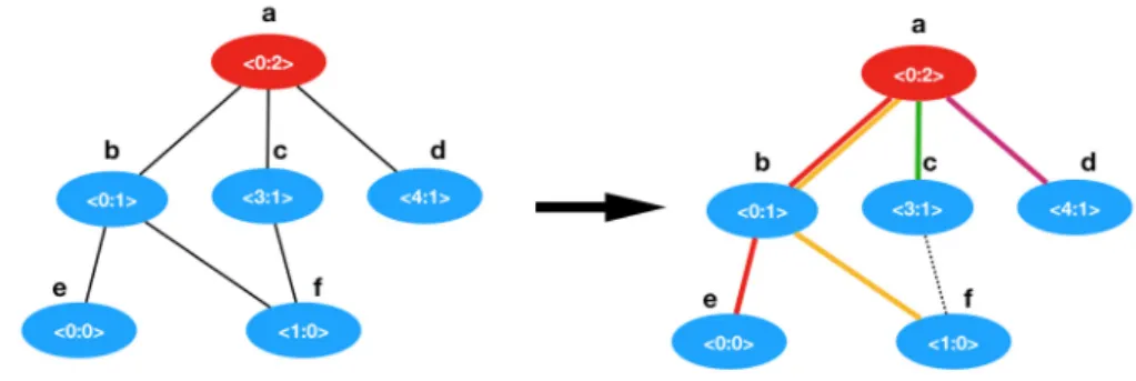
In Figure 4 is represented a network with six nodes V = {a, b, c, d, e, f }, each node with its own label < y : h >. Figure 5 shows the state transition of nodes according to Algorithm 1 while Figure 4, shows the path followed by the transmission of messages during the convergecast process. Note that nodes take different actions (send, listen or sleep) at different time slots. According to the y part of their labels, we identify four sets of nodes:

Nodes in group {a, b, e}, wake up at round 0 and begin to propagate their messages following the path e → b → a to the sink (a). This path is marked in red in Figure 4. Node {f }, wakes up at round 1 and sends its message using the path f → b → a to the sink, marked in yellow in Figure 4.

(19)

Node {c}, wakes up in round 3 and sends its message directly to the sink. The path is marked in green in Figure 4.

Node {d}, wakes up in round 4 and sends its message directly to the sink. The path is marked in purple in Figure 4.

Figure 4 Execution of Algorithm 1

Figure 5 shows the actions for each node in each time slot as per Algorithm 1. S, L, T represent the states Sleep, Listen and Send respectively (T stands for Transmit). States L and T in red represent an effective transmission. For example at time < 0 : 0 >, node e is in state Send and node b is in state Listen. Since they are directly connected (see Figure 4), the message from e can be received by node b. L in green means that the node is in state

Listen, but there is no incoming message to be received. For example at time < 0 : 2 >,

node e is in state Listen. However, there is no neighbor of e in state Send. Hence, e has nothing to receive. State T in green means that node can Send, but it has no message to send. For example at time < 1 : 0 >, node e is in state Send. However, e has already sent its message to b at time < 0 : 0 >.

(20)

C

Full-duplex Mode

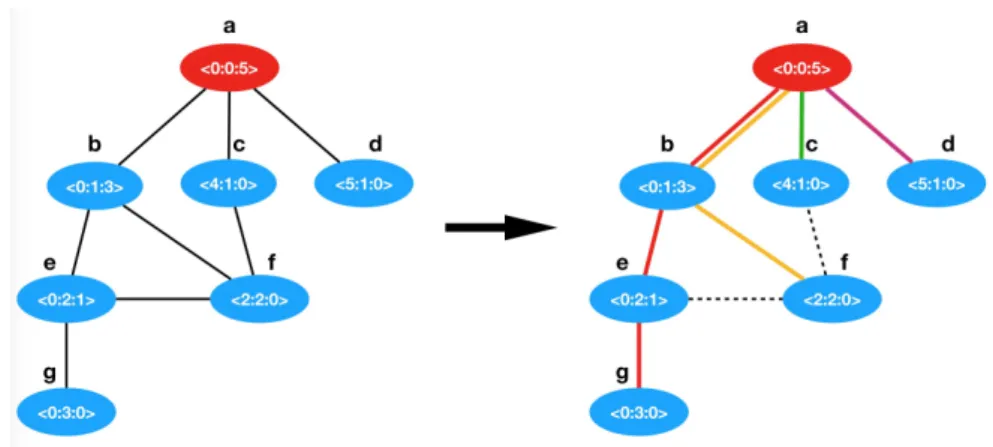
In the following we present an example for the execution of Algorithm 5. In Figure 6 is represented a network with seven nodes V = {a, b, c, d, e, f, g}, each node has its own label

< y : h : z >. By using Algorithm 5, nodes will have to execute different actions (Send, Listen, S&L or Sleep) at different time slots. Following their label, the seven nodes will be

separated into four group, according to the y field of their labels:

Nodes in the group {a, b, e, g} wake up at round 0 and begin to propagate their messages following the path g → e → b → a to the sink, marked on red in the figure. Node g wakes up only for 1 round. e wakes up for 2 rounds, b for 4 rounds and a for 6 rounds. Node {f } wakes up at round 2 and sends its message by passing the path f → b → a to the sink, marked on yellow in the figure. f wakes up for only 1 round.

Node {c} wakes up at round 4 and it sends its message directly to the sink, marked on green in the figure. c wakes up for only 1 round.

Node {d} wakes up at round 5 and sends its message directly to the sink, marked on purple in the figure. d wakes up for only 1 round.

Figure 6 Visualization of Algorithm 5

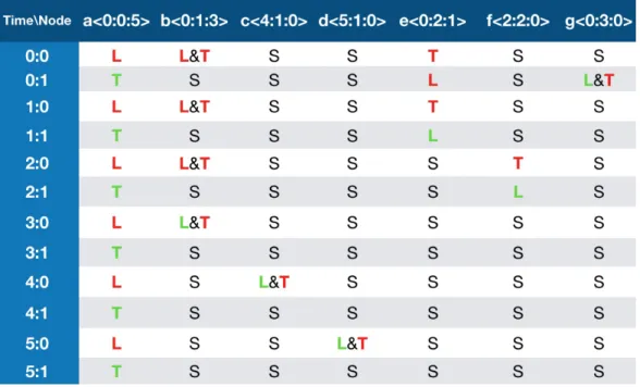
Figure 7 shows in details the actions for each node in each time slot. S, L, T and S&L represent the states Sleep, Listen, Send and S&L respectively. The states L and T in red mean that a transmission happens. L or T in green means that the node is in state Listen or Send, but there is no incoming message to be received or it has no message to send.

In this scenario, the sink has six messages to receive. From the figure, during each round from round 0 to round 5, the sink node a has always one effective Listen, that means at the end of round 5, the sink has already received six messages. As each message comes initially from a different node, the convergecast therefore succeeds in six rounds.

(21)