HAL Id: inria-00078183
https://hal.inria.fr/inria-00078183
Submitted on 3 Jun 2006
HAL is a multi-disciplinary open access
archive for the deposit and dissemination of sci-entific research documents, whether they are pub-lished or not. The documents may come from teaching and research institutions in France or abroad, or from public or private research centers.
L’archive ouverte pluridisciplinaire HAL, est destinée au dépôt et à la diffusion de documents scientifiques de niveau recherche, publiés ou non, émanant des établissements d’enseignement et de recherche français ou étrangers, des laboratoires publics ou privés.
FAIL-MPI: How fault-tolerant is fault-tolerant MPI ?
Thomas Herault, William Hoarau, Pierre Lemarinier, Eric Rodriguez,
Sébastien Tixeuil
To cite this version:
Thomas Herault, William Hoarau, Pierre Lemarinier, Eric Rodriguez, Sébastien Tixeuil. FAIL-MPI: How fault-tolerant is fault-tolerant MPI ?. [Research Report] 1450, 2006, pp.26. �inria-00078183�
FAIL-MPI:
How fault-tolerant is fault-tolerant MPI ?
Thomas Herault
William Hoarau
Pierre Lemarinier
Eric Rodriguez
S´ebastien Tixeuil
INRIA/LRI, Universit´e Paris-Sud, Orsay, France
E-mail: { herault, hoarau, lemarini, rodrigue, tixeuil }@lri.fr
phone: (+33) 1 69 15 4222
fax: (+33) 1 69 15 4213
RR LRI 1450
Abstract
One of the topics of paramount importance in the development of Cluster and Grid middleware is the impact of faults since their occurrence probability in a Grid infrastructure and in large-scale distributed system is actually very high. MPI (Message Passing Interface) is a popular abstraction for programming distributed computation applications. FAIL is an abstract language for fault occurrence description capable of expressing complex and realistic fault scenarios. In this paper, we investigate the possibility of using FAIL to inject faults in a fault-tolerant MPI implementation. Our middleware, FAIL-MPI, is used to carry quantitative and qualitative faults and stress testing.
1
Introduction
A long trend in the high performance distributed systems is the increase of the number of nodes. As a consequence, the probability of failures in supercomputers and distributed systems also increases. So fault tolerance becomes a key property of parallel applications. Designing and implementing fault tolerant software is a complex task. Fault tolerance is a strong property which implies a theoretical proof of the underlying protocols. The protocol implementation should then be checked with respect to the specification.
In order to validate this implementation, a rigorous testing approach can be used. Au-tomatic failure injection is a general technique suitable for evaluating the effectiveness and robustness of the distributed applications against various and complex failure scenarios.
After having validated the fault tolerant implementation, it is necessary to evaluate its performance, in order to adapt the best protocol suitable for an actual distributed system. Fault-Tolerant distributed applications are classically evaluated without failures. However, performances under a failure-prone environment is also a significant information to evaluate and tune a fault-tolerant distributed system. Automatic failure injection is desirable to evaluate fairly different heuristics or parameters under the same failure conditions.
In this paper, we present FAIL-MPI, a software that can be used both for software fault-injection and for stress testing of distributed applications, which are the basis for dependability benchmarking in distributed computing. As a case study for complex fault tolerant system, we strain the MPICH-Vcl non-blocking implementation of the Chandy-Lamport protocol. MPICH-Vcl is a high performance fault tolerant MPI library which provides a generic framework to add transparently the fault tolerance property to any MPI application.
2
FAIL-FCI: a fault injection tool
2.1
Previous works
The issues for testing component-based distributed systems have already been described and methodology for testing components and systems has already been proposed. [THS06] presents a thorough survey of the available tools. However, testing for fault tolerance remains a challenging issue. Indeed, in production systems, the fault-recovery code is rarely executed in the test-bed as faults rarely get triggered. As the ability of a system to perform well in the presence of faults depends on the correctness of the fault-recovery code, it is mandatory to actually stress this code. Testing based on injection can be used to test for fault-tolerance by injecting faults into a system under test and observing its behavior. The most obvious point is that simple tests (e.g. every few minutes or so, a randomly chosen machine crashes) should be simple to write and deploy. On the other hand, it should be possible to inject faults for very specific cases (e.g. in a particular global state of the application), even if it requires a better understanding of the tested application. Also, decoupling the fault injection platform from the tested application is a desirable property, as different groups can concentrate on different aspects of fault-tolerance. Decoupling requires that no source code modification of the tested application should be necessary to inject faults. This also increase the reliability of the test, since the code tested is the actual implementation that will be run in a production environment. Finally, to properly evaluate a distributed application in the context of faults, the impact of the fault injection platform should be kept low, even if the number of machines is high. Of course, the impact is doomed to increase with the complexity of the fault scenario, e.g. when every action of every processor is likely to trigger a fault action, injecting those faults will induce an over-head that is certainly not negligible. The table below captures the major differences between the main solutions for distributed fault injection relatively to those criteria.
Criteria NFTAPE[Sa00] LOKI [CLCS00] FAIL-FCI High Expressiveness yes no yes High-level Language no no yes Low Intrusion yes yes yes Probabilistic Scenario yes no yes No Code Modification no no yes Scalability no yes yes Global-state Injection yes yes yes
2.2
FAIL-FCI
We now describe briefly the FAIL-FCI framework that is fully presented in [HT05]. First, FAIL (for Fault Injection Language) is a language that permits to easily describe fault scenarios. Second, FCI (for FAIL Cluster Implementation) is a distributed fault injection platform whose inputs language for describing fault scenarios is FAIL. A scenario describes, using a high-level abstract language, state machines which model fault occurrences. The FAIL language also describes the association between these state machines and a computer (or a group of computers) in the network.
The FCI platform is composed of several building blocks:
The FCI compiler : The fault scenarios written in FAIL are pre-compiled by the FCI
com-piler which generates C++ source files and default configuration files.
The FCI library: The files generated by the FCI compiler are bundled with the FCI library
into several archives, and then distributed across the network to the target machines according to the user-defined configuration files. Both the FCI compiler generated files and the FCI library files are provided as source code archives, to enable support for heterogeneous clusters.
The FCI daemon: The source files that have been distributed to the target machines are
in the system. Those executables are referred to as the FCI daemons. When the experiment begins, the distributed application to be tested is executed through the FCI daemon installed on every computer, to allow its instrumentation and its handling according to the fault scenario.
3
MPICH-V: Fault Tolerant MPI
MPI (Message Passing Interface) is a standard for programming parallel applications using message passing systems. Thanks to its high availability on parallel machines from low cost clusters to clusters of vector multiprocessors, it allows the same code to run on different kind of architectures. It also allows the same code to run on different generations of machines, ensuring a long life time for the code. Moreover, MPI conforms to popular high performance, message passing, programming styles. Even if many applications follow the SPMD program-ming paradigm, MPI is often used for Master-Worker execution, where MPI nodes play different roles. These three parameters make MPI a first choice programming environment for high performance applications. MPI in its specification [SOHL+96] and most deployed
implementations (e.g. MPICH [GLDS96]) follows the fail stop semantic (specification and implementations do not provide mechanisms for fault detection and recovery). Thus, MPI applications running on a large cluster may be stopped at any time during their execution due to an unpredictable failure.
The need for fault tolerant MPI implementations has recently reactivated the research in this domain. Several research projects are investigating fault tolerance at different levels: network [SSB+03], system [BCH+03], applications [FD00]. Different strategies have been
proposed to implement fault tolerance in MPI: a) user/programmer detection and manage-ment, b) pseudo automatic, guided by the programmer and c) fully automatic/transparent. For the last category, several protocols have been discussed in the literature. As a conse-quence, for the user and system administrator, there is a choice not only among a variety of
fault tolerance approaches but also among various fault tolerance protocols.
The best choice of fault tolerance protocol depends highly on the number of components, the communication scheme for the parallel application, and the system behavior with respect to failures. In this work, we strain the Chandy-Lamport implementation of the MPICH-V project [HLBC] with high failure rates, in order to define its fault tolerance capabilities.
The Chandy-Lamport algorithm [CL85] proposes to implement fault-tolerance through a coherent snapshot / rollback recovery protocol. During the execution, components can trigger checkpoint waves, which build a coherent view of the distributed application. Each process saves its image on a reliable media when entering the coherent view. When a process is subject to failure, the distributed application is interrupted, computing resources are allocated to replace the failed processes, and all processes rollback, that is load their last checkpoint image that is member of a complete coherent view. Since the view builds a possible distributed configuration of the application, the execution of the application can pursue from this point on, according to the original specification, as if failures did not hit the system.
The MPICH-V [HLBC] project aims at comparing the performances of different fault tolerance protocols in the MPI implementation mpich-1 [GLDS96]. One of the protocol im-plemented is the non-blocking Chandy-Lamport algorithm with optimizations. There are two possible implementations of the Chandy-Lamport algorithm: blocking or non-blocking. The blocking implementation uses markers to flush the communication channels and freezes the communications during a checkpoint wave. On the contrary, the non-blocking implemen-tation let the application continue during a checkpoint wave and store the messages emitted before a wave marker in the checkpoint image. We describe more thoroughly the protocol and its implementation below, but the capacity of storing a message in transit lead us to implement a MPI process with two separate components, running each in a unix process: a computation process (MPI) and a communication process (daemon). The communication process is used to store in-transit messages and to replay these messages when a restart is
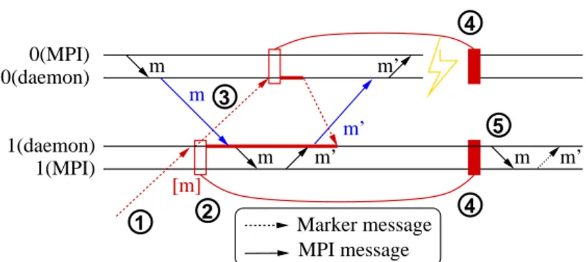
performed. 1 3 4 5 2 4 MPI message Marker message m m’ m 0(daemon) 0(MPI) 1(MPI) 1(daemon) m m’ m m’ [m] m’
Figure 1: A PMI application execution on MPICH-Vcl with one fault
The protocol works as shown in the figure 1. The MPI process 1 initially receives the marker from the checkpoint scheduler (1), stores its local state (2) and sends marker to every process (2). From this point, every message, like m in the figure, received after the local checkpoint and before having received the marker of the sender, is stored by the daemon process. When the MPI process 0 receives the marker, it starts its local checkpoint and sends a marker to every other process (3). The reception of this marker by process 1 concludes its local checkpoint. If a failure occurs, all processes restart from their last stored checkpoint (4) and the daemon process replays the delivery of the stored messages (5). Note that the message m′ may be not sent again in the new execution.
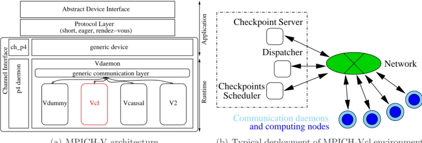
MPICH implements a full MPI library from a channel. Such a channel implements the basic communication routines for a specific hardware or for a new communication protocols. We developed a generic framework, called MPICH-V, to compare different fault tolerance protocols for MPI applications. This framework implements a channel for the MPICH 1.2.7 library, based on the ch p4 default channel.
MPICH-V is composed of a set of runtime components and a channel called ch v. This channel relies on a separation between the MPI application and the actual communication system. Communication daemons (Vdaemon) provide all communication routines between the different components involved in MPICH-V. The fault tolerance is performed by
imple-ch_p4
p4 daemon
Channel Interface
Application
Abstract Device Interface Protocol Layer (short, eager, rendez−vous)
generic device Vdaemon generic communication layer
Runtime
Vdummy Vcl Vcausal V2
(a) MPICH-V architecture
Dispatcher Checkpoints Scheduler Network Checkpoint Server Communication daemons and computing nodes
(b) Typical deployment of MPICH-Vcl environment
Figure 2: MPICH-V architecture and typical deployment
menting hooks in relevant communication routines. This set of hooks is called a V-protocol. The V-protocol of interest for this paper Vcl, which is a non-blocking impletation of the Chandy-Lamport algorithm.
Daemon A daemon manages communications between nodes, namely sending, receiving, reordering and establishing connections. It opens one TCP socket per MPI process and one per server type (the dispatcher and a checkpoint server for the Vcl implementation). It is implemented as a mono-threaded process that multiplexes communications through
select calls. To limit the number of system calls, all communications are packed using iovec
techniques. The communication with the local MPI process is done using blocking send and receive on a Unix socket.
Dispatcher The dispatcher is responsible for starting the MPI application. It starts the different processes and servers first, then MPI processes, using ssh to launch remote processes. The dispatcher is also responsible for detecting failures and restarting nodes. A failure is assumed after any unexpected socket closure.
Failure detection relies on the Operating System TCP keep-alive parameters. Typical Linux configurations define a failure detection as a miss of 9 consecutive losses of keep-alive probes, where keep-alive probes are expected every 75 seconds. These parameters can be
changed to provide more reactivity to hard system crashes. In this work, we emulated failures by killing the task, not the operating system, so failure detection was immediate, and the TCP connection was broken as soon as the task was killed by the operating system.
Checkpoint server and checkpoint mechanism The two implementations use the same abstract checkpointing mechanism. This mechanism provides a unified API to address three system-level task checkpointing libraries, namely Condor Standalone Checkpointing Library [LTBL97], libckpt [Zan05] and the Berkeley Linux Checkpoint/Restart [JD03, SSB+03]. All
these libraries allow its user to take a unix process image in order to store it on a disk and to restart this process on the same architecture. By default, BLCR, which is the most up-to-date library, is used.
The checkpoint servers are responsible for collecting local checkpoints of all MPI pro-cesses. When a MPI process starts a checkpoint, it duplicates its state by calling the fork system call. The forked process calls the checkpoint library to create the checkpoint file while the initial MPI process can continue the computation. The daemon associated with the MPI process connects to the checkpoint server that first creates a new process responsible for managing the checkpoint of this MPI process. Then 3 new connections are established (data, messages and control) between the daemon and the server. The clone of the MPI process writes its local checkpoint in a file, and the daemon pipelines the reading and the sending of this file to the checkpoint server using the data connection. When the checkpoint file has been completely sent, the clone of the MPI process terminates and the daemon closes the data connection: then it sends the total file size using the control connection. Every message to be logged according to the Chandy and Lamport algorithm is temporary stored in the volatile memory of the daemon in order to be sent to the checkpoint server in the same way using the message connection. Using this technique, the whole computation is never interrupted during a checkpoint phase.
checkpoints. Thus, checkpoint servers only store one complete global checkpoint at a time using two files alternatively to store the current global checkpoint and the last complete one. If a failure occurs, all MPI processes restart from the local checkpoint stored on the disk if it exists: otherwise they obtain it from the checkpoint server.
Checkpoint Scheduler The checkpoint scheduler manages the different checkpoint waves. It regularly sends markers to every MPI process. The checkpoint frequency is a parameter defined by the user. It then waits for an acknowledgment of the end of the checkpoint from every MPI process before asserting the end of the global checkpoint to the checkpoint servers. The checkpoint scheduler starts a new checkpoint wave only after the end of the previous one.
4
FAIL-MPI: merging self-deploying tools
The previously available FAIL-FCI fault-injection platform [HT05] made several assump-tions about the distributed application that are not valid in the self-deploying MPICH-V. Specifically, it was assumed that a ssh-like mechanism was systematically used to launch a process in the distributed application. Then, the FAIL-FCI middleware was able to control the launch, suspend, resume, and stop actions by using GDB with a command line interface. As MPICH-V is also a middleware that self-deploys itself on many nodes, it was not possible to deploy MPICH-V inside FAIL-FCI.
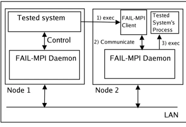
To circumvent this problem, we developed a new integration scheme for fault injection that can be used for any self-deploying distributed application: FAIL-MPI. The major dif-ference between FAIL-FCI and FAIL-MPI is that the former does not require any change on the application under test, while the latter provides an interface for self-deploying ap-plication, that they can use to support fault injection. Not using this interface means that the self-deploying application will suffer no fault, while using the interface triggers the use of the fault scenario that was designed, as in the FAIL-FCI middleware. The basic scheme
Figure 3: FAIL-MPI integration scheme
is as follows: instead of simply launching a new process by running a command line argu-ment, the self-deploying application registers itself with a FAIL-MPI daemon. Of course, the FAIL-MPI daemon is expected to already run on the machine. Also, it is possible to automate this scheme so that the change in the source code is almost transparent, e.g. by having the command line argument replaced by a script that effectively makes the call to the FAIL-MPI daemon. Then, the FAIL-MPI daemon manages the application specified by the command line through a debugger to inject fault actions. Figure 3 captures this behavior.
Another new feature of FAIL-MPI is the ability to attach to a process that is already running, so that processes that were not created from a command line argument (such as those obtained by fork system calls) can also be used in the FAIL-MPI framework. This requires simply to register with the FAIL-MPI daemon using the process identifier as an argument, so that it can attach to the running process.
By these two extensions, it is possible that the application under test is not launched by the FAIL-MPI middleware (e.g. this happens in peer to peer systems or desktop grids, where new users are expected to join the system on a regular basis), yet a fault scenario would typically need to perform action when new processes join or leave the system. One obvious reason for this is that we should inject faults only on processes that are actually running, but also that one can be interested in what happens when a process crash and a process join occur simultaneously. As a result of the above observation, we integrated three
new FAIL triggers (i.e. model for system events) in the FAIL language:
1. onload: this trigger occurs when a process joins the distributed application under test,
2. onexit: this trigger occurs when a process exits normally the distributed application under test,
3. onerror: this trigger occurs when a process exists abnormally the distributed appli-cation under test.
5
Performance Evaluation
In this section, we strain the MPICH-Vcl implementation with many patterns of failures and analyze the observed performance. For all measurement, We used the NAS parallel BT (Block Tridiagonal) benchmark [BHS+95] class B with varying number of nodes. This
bench-mark provides complex communication schemes and is suitable for testing fault tolerance. The class B ensures a medium sized memory footprint and is suitable for measurements in a reasonable time.
We ran the measurements on Grid Explorer, a component of the Grid5000 platform. Grid5000 is an experimental platform dedicated to computer science for the study of grid algorithms, and partly founded by the French incentive action “ACI Grid”. Grid5000 as of today consists in 13 clusters located in 9 french towns with 40 to 450 processors each, gathering 1928 processors in total. Grid Explorer is a major component of the Grid5000 platform. It is located at Orsay and consists in 216 IBM eServer 325 computers. All com-puters are dual-processor AMD Opterons running at 2.0 GHz with 2 GB of RAM, 80 GB IDE hard drive and a GigaEthernet network interface card. A major feature of the Grid5000 project is the ability for the user to deploy its own environment (including operating system kernel and distribution) over all nodes that are dedicated to the experiment. We deployed a Linux operating system, version 2.6.13-5, including the BLCR module version 0.4.2 for
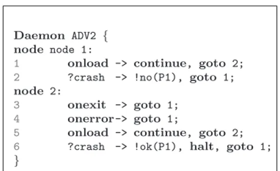
Daemon ADV2 { node node 1:
1 onload -> continue, goto 2; 2 ?crash -> !no(P1), goto 1; node 2:
3 onexit -> goto 1; 4 onerror-> goto 1;
5 onload -> continue, goto 2; 6 ?crash -> !ok(P1), halt, goto 1; }
Figure 4: FAIL-MPI scenario for every MPI computing nodes
checkpointing. We compiled the benchmarks with g77 from the FSF version 4.1.0 and the usual optimization options (-O3).
To implement the various failure scenarios, we used a centralized approach. We designed a specific FAIL-MPI daemon using the FAIL language to coordinate failure injection while the other FAIL-MPI daemons control the execution of MPI computing nodes. The specific FAIL-MPI daemon is denoted as “P1” in the remaining of the paper. For all measurements, P1 chooses a process subject to failure according to the failure scenario, and sends a failure order to the controlling FAIL-MPI daemon. When a daemon receives a failure order, either a MPI node is actually running on it, or not. If there is such a MPI node, the failure is injected and P1 receives an acknowledgement; if there is no MPI node, P1 receives a negative acknowledgement and may choose another node to inject the failure.
Formally, the FAIL scenario used for controlling every MPI computation node is given in Figure 4. Each FAIL-MPI daemon has two states; in state 1, it awaits for the onload event to go to state 2. If a crash order is received (line 2), it sends the negative acknowledgement and remains in state 1. In state 2, if the MPI node exits or is subject to an error, it goes back in state 1 to wait for a new MPI node to register. When receiving a crash order (line 6), it sends the acknowledgement, halt the process and goes back to state 1.
Some of the experiments introduce too much stress into the application and the fault tolerant library is not able to tolerate that level of stress. Then, the application either freezes or enters a cycle of rollback / crash. If the application cycles between rollback and
crashes, this denotes a level of failure too high for having any progression of the computation. If the application freezes, this denotes a bug in the implementation (as would an execution terminating before the finalization). For detecting both cases, we introduced a timeout on all our experiments. After 1500 seconds, every component of the application (including checkpoint servers, scheduler and dispatcher) is killed and the experiment is marked as non terminating.
In every experiment, we distinguish between experiments that do not progress anymore due to the high failure frequency (when the failure frequency is too high, the application has no time to reach the next checkpoint wave before being hurt by a new failure, so it cannot progress and appears to stall) and experiments that do not progress due to a bug in the fault tolerant implementation. The difference between the two kinds of experiments is done by analysing the execution trace. In the subsequent figures, we present the non progressing execution percentages with a green bar and the buggy execution percentages with a red bar.
5.1
Impact of faults frequency
Figure 5 presents the impact of fault frequency on the performances of the BT class B benchmark for 49 processes. 53 machines were devoted to this run, ensuring that enough spare processors were found, whatever the number of failures.
The scenario, presented in Figure 5(a), injects failures at a given rate. The algorithm for the daemon P1 is the following: A process is first randomly (and uniformly) chosen (line 1), then a timeout is programmed (line 2). Upon expiration of the timeout (line 3), the failure injection order is sent to the chosen process. If an acknowledgement is received, a new process is randomly chosen and the cycle continues (line 5). If a negative acknowledgement is received (denoting that no MPI process is running on the same node as the chosen process, which can happen because of previous failure injections), another process is immediately chosen (line 4) and a failure injection order is immediately sent to the new process (line 6), until an acknowledge is eventually received.
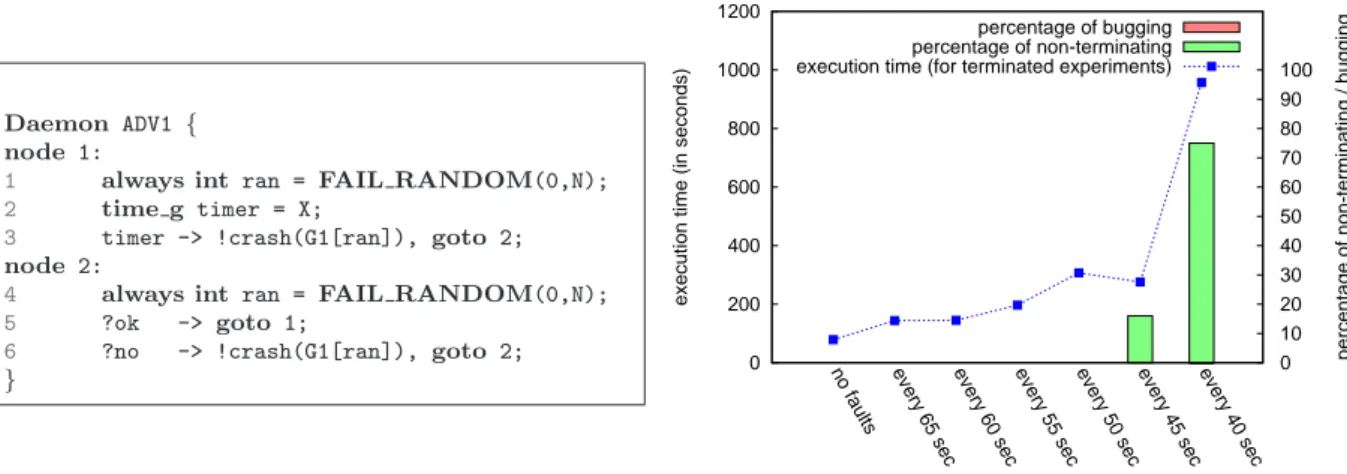
Daemon ADV1 { node 1:
1 always int ran = FAIL RANDOM(0,N); 2 time g timer = X;
3 timer -> !crash(G1[ran]), goto 2; node 2:
4 always int ran = FAIL RANDOM(0,N); 5 ?ok -> goto 1;
6 ?no -> !crash(G1[ran]), goto 2;
} 0 200 400 600 800 1000 1200 100 90 80 70 60 50 40 30 20 10 0
execution time (in seconds)
percentage of non-terminating / bugging
no faults every 65 sec every 60 sec every 55 sec every 50 sec every 45 sec every 40 sec percentage of bugging percentage of non-terminating execution time (for terminated experiments)
(a) Scenario of P1 (b) Execution time and percentage of non-terminating experiments
Figure 5: Impact of faults frequency
The performance measurements are presented in Figure 5(b). The blue line represents the total execution time of the benchmark as function of the frequency of faults; the percentage of non-terminating experiments according to the same parameter is represented using green bars and the percentage of bugging experiments is presented using red bars. Every experiment was run 6 times and the value presented here is the average value of the measures.
As the scenario describes it, no overlapping faults were intended in this experiment, and we can see that there are no buggy executions. At some point, the time between two faults is less than the time between two checkpoints, and when this happens, the application has not enough time to progress. Non-terminating executions appears, and progress with the frequency of failures, up to a point where almost no execution terminates. Similarly, the rollback/recovery algorithm takes an increasing part of the total execution when the number of faults per minute increases, and we can see with the green line that the execution time progresses with the number of faults per minute. This is partly contradicted by the measurement for one failure every 45s. Tighter analysis of the experiment traces demonstrate that for this frequency of failures, failures occur just after checkpoint waves (this is due to the checkpoint wave frequency set at one checkpoint wave every 30s). When failures occur just after a checkpoint wave, the rollback/recovery mechanism is the most efficient.
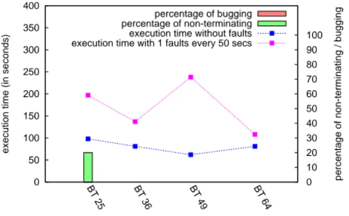
0 50 100 150 200 250 300 350 400 100 90 80 70 60 50 40 30 20 10 0
execution time (in seconds)
percentage of non-terminating / bugging
BT 25 BT 36 BT 49 BT 64 percentage of bugging percentage of non-terminating execution time without faults execution time with 1 faults every 50 secs
Figure 6: Impact of scale
5.2
Impact of scale
Figure 6 presents the impact of the scale on the performance of the BT class B benchmark for a given frequency of fault injection. In this experiment, one fault was injected every 50 seconds and the number of nodes running the application varies from 25 to 64 (BT needs a natural square number of nodes). The FAIL scenario is the same as the one used in the previous experiment (see Figure 5(a)). Each experiment was run 5 times and the average value is presented here.
At 25 nodes, one of the five experiments was non-terminating. Every experiment are run with the same number of checkpoint servers. Since BT use an approximately constant memory fingerprint divided equally between the computing nodes, at 25 nodes, the size of each checkpoint image is greater than at 36 or more nodes. So each checkpoint image transfer individually takes more time at 25 nodes than at the other sizes. This implies that the checkpoint and recovery times are longer for 25 nodes than the other sizes, and for one of the experiments, the checkpoint waves were synchronized (per chance) with the failure injection (every 50s). So there was no progression anymore. When the checkpoint image size decreases and the checkpoint and recovery times also decrease, this phenomenon appears with lower probability.
The total execution time measured for the experiments with a failure injected every 50s at different sizes is apparently chaotic. It can be very close to the time measured without failure (at 64 nodes) or up to 2.5 times slower. In fact, a precise analysis of the measurements demonstrates that the variance for these measurement increases with the number of nodes, and the average value presented here is not meaningful. Failure injection at regular period of times disregard the protocol, and failures injected just before a checkpoint wave have a major impact on the overall performances, while failures injected just after a checkpoint wave have an impact almost non-measurable on the performances.
In order to provide a significant measure according to this parameter, the number of experiments to run would be extremely high. Another solution is to precisely measure the date of failure injection as compared to the date of the last checkpoint wave, and measure the impact of this delay on the total execution time. However, this also implies to be able to read the variables of the program strained, which is a planned feature of FAIL-MPI, but is not yet implemented.
5.3
Impact of simultaneous faults
Figure 7 presents the impact on the performance of the BT class B benchmark for 49 processes of the number of simultaneous faults appearing every 50 seconds. This measurement is a stress test for the fault tolerant MPI implementation with rare cases of simultaneous faults. The fault injection scenario is formally given in Figure 7(a) and Figure 7(b) presents the percentage of buggy experiments and the average total execution time for 6 experiments.
The scenario is a simple variation of the previous one. At timeout expiration, not one, but X (X being the abscissa of the figure) processes are chosen, one after the other, to crash. Every time the master enters the node 1, it uniformly selects a process (line 2), then at timer expiration (line 4) it sends the crash order to the selected process and enters the node 2. Every time the process enters node 2, it select another process (line 5). In node 2, if it receives the positive acknowledgement and there are still faults to inject (line 6), it sends
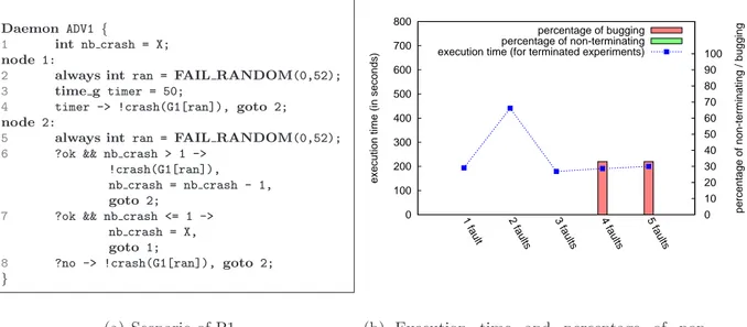
Daemon ADV1 {
1 int nb crash = X; node 1:
2 always int ran = FAIL RANDOM(0,52); 3 time g timer = 50;
4 timer -> !crash(G1[ran]), goto 2; node 2:
5 always int ran = FAIL RANDOM(0,52); 6 ?ok && nb crash > 1 ->
!crash(G1[ran]), nb crash = nb crash - 1, goto 2;
7 ?ok && nb crash <= 1 -> nb crash = X, goto 1;
8 ?no -> !crash(G1[ran]), goto 2; } 0 100 200 300 400 500 600 700 800 100 90 80 70 60 50 40 30 20 10 0
execution time (in seconds)
percentage of non-terminating / bugging
1 fault 2 faults 3 faults 4 faults 5 faults percentage of bugging percentage of non-terminating execution time (for terminated experiments)
(a) Scenario of P1 (b) Execution time and percentage of non-terminating experiments
Figure 7: Impact of simultaneous faults
the crash order to the selected process, decrements the number of faults to inject and enters the node 2 again. If a negative acknowledgement is received (line 8), another process is selected by re-entering the node 2. When all failures have been injected successfully (line 7), the number of failures to inject next time is reset to X and P1 enters the node 1, thus programming a new timeout.
One can see that at 5 or 6 simultaneous fault injections every 50s, one third of the ex-periments had a buggy behavior. A complete analysis of the execution trace demonstrated that all of them where frozen during the recovery phase after a fault injection. This phe-nomenon does not appear spontaneously with less simultaneous faults, and a majority of the executions were not subject to this behavior, even with multiple checkpoint phases and recovery phases (a checkpoint wave every 30s, so an average number of checkpoint waves between 6 and 7, and a failure injection every 50s, so approximately 4 faults and recovery per executions).
Bug hunting using FAIL-MPI In order to locate precisely the bug in MPICH-Vcl with FAIL-MPI, we conducted a set of experiments targeting more precisely this behavior. Since
Daemon ADV1 { node 1:
1 always int ran = FAIL RANDOM(0,52); 2 time g timer = 50;
3 timer -> !crash(G1[ran]), goto 2; node 2:
4 always int ran = FAIL RANDOM(0,52); 5 ?ok -> goto 3;
6 ?no -> !crash(G1[ran]), goto 2; node 3:
7 ?waveok -> !crash(FAIL SENDER), goto 4; node 4:
}
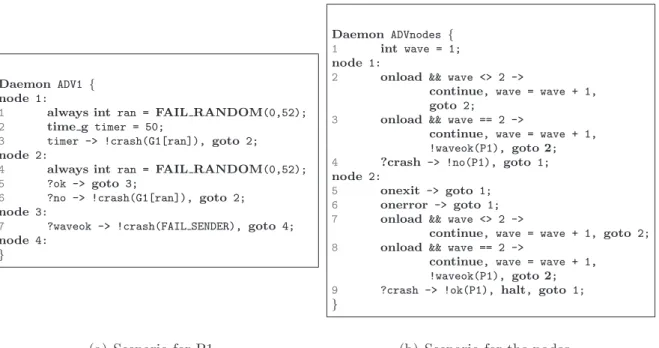
Daemon ADVnodes { 1 int wave = 1; node 1:
2 onload && wave <> 2 ->
continue, wave = wave + 1, goto 2;
3 onload && wave == 2 ->
continue, wave = wave + 1, !waveok(P1), goto 2; 4 ?crash -> !no(P1), goto 1; node 2:
5 onexit -> goto 1; 6 onerror -> goto 1; 7 onload && wave <> 2 ->
continue, wave = wave + 1, goto 2; 8 onload && wave == 2 ->
continue, wave = wave + 1, !waveok(P1), goto 2; 9 ?crash -> !ok(P1), halt, goto 1; }
(a) Scenario for P1 (b) Scenario for the nodes
Figure 8: FAIL scenario for the impact of synchronized faults
the execution trace suggested that the bug occurs at recovery time, we first designed a scenario to inject failures during this time. The scenario we used is formally given in figure 8. There are two scenarios, one for Process P1 (figure 8(a)), the other for the computing nodes (figure 8(b)). The complexity of the scenario imposes to modify the generic scenario used for the computing nodes. Roughly speaking, The algorithm for the daemon P1 is nearly the same than the one used for the fault frequency experiments. Lines 1 to 6 are used to ensure that the first fault is really injected (since we devoted more machines than needed to the experiment, in order to have spare nodes, a participating node may not be executing any MPI daemon and the positive acknowledge must be checked to ensure that a failure is indeed injected). Then, the P1 daemon waits for a message from a computing node FAIL-MPI daemon which denotes the beginning of a recovery wave, and send him a crash order (line 7). After sending this order it goes in an empty state (node 4) and do not inject any other faults during the execution.
In order to detect a recovery wave, the nodes are subject to the control of the MPI daemon of Figure 8(b). Initially, the wave counter is set to 1, and the onload event is used to count
0 50 100 150 200 250 300 350 400 100 90 80 70 60 50 40 30 20 10 0
execution time (in seconds)
percentage of non-terminating / bugging
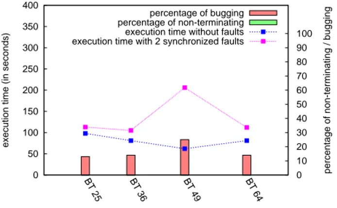
BT 25 BT 36 BT 49 BT 64 percentage of bugging percentage of non-terminating execution time without faults execution time with 2 synchronized faults
Figure 9: Impact of synchronized faults
the number of recovery waves. Since the MPICH-Vcl runtime will halt every communication daemon when a failure occurs and then relaunch a daemon on each node, this event denotes first the initial launch, then recovery waves. So, at first, a communication daemon is subject to the node 1 behavior, which counts the number of communication daemon launches. When this number is 2, the daemon is in the first recovery wave, so a waveok message is sent to the P1 process and the FAIL daemon enters node 2. On node 2, the behavior is the same as in the previous experiments, and when the FAIL daemon receives the crash orders, it halts the controlled process.
The performance measurements are presented in Figure 7(b). We can note that even if we injected only 2 faults using this scenario, for every scale, some experiments did not terminate due to a bug in the fault tolerant implementation. This demonstrate that the bug is located in this part of the execution and is not a consequence of the size of the application. However, a large majority of the executions is not subject to the bug, so we have to define more precisely the conditions for failure injection. At this step, we suspected that the recovery bug happens only if a process is subject to failure while it is in a recovery wave, some of the other processes have not finished terminating their execution because of the failure detection, and the MPICH-Vcl dispatcher detects the failure of the process in the new wave. It seems that if this happens, it becomes confused between which processes are
Daemon ADV1 { node 1:
1 always int ran = FAIL RANDOM(0,52); 2 time g timer = 50;
3 timer -> !crash(G1[ran]), goto 2; node 2:
4 always int ran = FAIL RANDOM(0,52); 5 ?ok -> goto 3;
6 ?no -> !crash(G1[ran]), goto 2; node 3:
7 ?waveok -> !crash(FAIL SENDER), goto 4; node 4:
8 ?waveok -> !nocrash(FAIL SENDER), goto 4; }
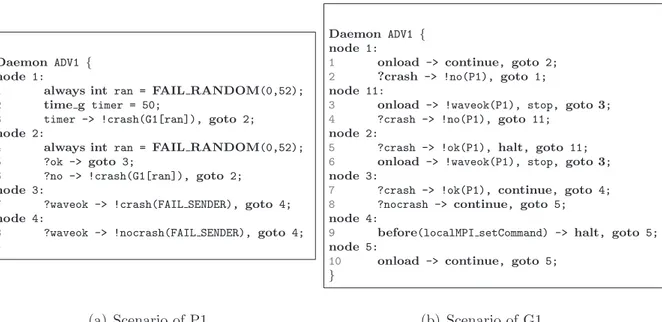
Daemon ADV1 { node 1:
1 onload -> continue, goto 2; 2 ?crash -> !no(P1), goto 1; node 11:
3 onload -> !waveok(P1), stop, goto 3; 4 ?crash -> !no(P1), goto 11;
node 2:
5 ?crash -> !ok(P1), halt, goto 11; 6 onload -> !waveok(P1), stop, goto 3; node 3:
7 ?crash -> !ok(P1), continue, goto 4; 8 ?nocrash -> continue, goto 5; node 4:
9 before(localMPI setCommand) -> halt, goto 5; node 5:
10 onload -> continue, goto 5; }
(a) Scenario of P1 (b) Scenario of G1
Figure 10: FAIL scenario for the impact of synchronized faults based on MPI state
in which state and which should be restarted.
In order to demonstrate this, we conceived the last scenario presented in Figure 10. In this experiment, we wanted to run the same scenario than the one used in the previous experiment but using the state of the MPI daemon to determinate the position when the second fault is injected. Because we need to ensure that the MPICH-Vcl dispatcher is confused with the state of the process in the recovery wave, we need to inject the failure after the connection is established and some of the initial communications are done. So, the second fault is injected just before the MPI communication daemon calls the function localMPI_setCommand. This function is called by the communication daemon after it exchanged the initial arguments with the dispatcher, and this ensures that the dispatcher sees this daemon as running, so will trigger the failure detection mechanism when the failure occurs.
The specific FAIL-MPI daemon (P1) used to coordinate the failure injection is described in Figure 10(a). The only modification with the previous scenario is that while in the node 4, process P1 sends nocrash orders, so that the computing processes will not be blocked when entering the localMPI_setCommand function. The FAIL-MPI daemons behaviors (G1) controlling the execution of each MPI computing node are described in Figure 10(b). The
0 50 100 150 200 250 300 350 400 100 90 80 70 60 50 40 30 20 10 0
execution time (in seconds)
percentage of non-terminating / bugging
BT 25 BT 36 BT 49 BT 64 percentage of bugging percentage of non-terminating execution time without faults execution time with state synchronized faults
Figure 11: Impact of synchronized faults depending on MPI state
algorithm for Daemon P1 is nearly the same than the on used in the previous experiments. Only the “node 4” has been modified, because after sending a crash order to the first daemon which detected an execution of a MPI daemon from the recovery wave, the daemon P1 must still wait for the message from every other daemon of the second wave to send them the order to continue their execution (line 8). Then, only the process receiving the crash order enters the node 4 where it will inject the failure just before entering Function localMPI_setCommand (line 9).
The corresponding measurements are presented in Figure 11. In every case, every exper-iment froze during the recovery wave. So, we conclude that the bug in the recovery process illustrated by the simultaneous failure injection appears when the dispatcher detects a failure of a process already recovered, while there are still other processes in the previous execution wave that did not received the termination order.
6
Conclusion
In this paper, we use the FAIL-MPI automatic fault injection tool to strain the MPICH-Vcl non-blocking implementation of the Chandy-Lamport protocol. We present the tool derived from the previous available FAIl-FCI fault injection tool, and evaluate the fault tolerance
properties of MPICH-Vcl through many experiments using the NAS bt benchmark in the MPICH-Vcl framework.
FAIL-MPI is the first version of FAIL that allows the application under test to dynam-ically launch and stop processes during the execution. For this purpose, we added specific new events to the FAIL language (namely spawning of a process, exit or interrution). Using this tool, we were able to reproduce automatically previous measurements that were done manually, like the impact of fault frequency on the execution time [LBH+04]. This provides
the opportunity to evaluate many different implementations at large scales and compare them fairly under the same failure scenarios.
The execution time measurements demonstrated a high variability depending on the time elapsed between the last checkpoint wave and the fault injection. In order to provide lower variance in the results, the FAIL language and FAIL-MPI tool shoul dbe able to read and modify internal variables of the stressed application: this is a planned feature.
The last experiments of the paper demonstrate the high expressivity of FAIL-MPI to precisely locate a rare bug in the dispatcher of MPICH-Vcl. We were able to demonstrate that if a second failure hits a process already recovered after it registered with the dispatcher, and other processes are still being stopped by the first failure detection, then the dispatcher is confused about the state of each process and forgets to launch at least one computing node. This bug is now corrected in the MPICH-Vcl framework and was discovered during this work.
FAIL-MPI is a valuable tool for detecting and situating bugs, and to evaluate the per-formance of a complex fault tolerant distributed system under precise failure conditions.
References
[BCH+03] Aur´elien Bouteiller, Franck Cappello, Thomas H´erault, G´eraud Krawezik, Pierre Lemarinier, and Fr´ed´eric Magniette. MPICH-V2: a fault tolerant MPI for
volatile nodes based on pessimistic sender ba sed message logging. In High
Performance Networking and Computing (SC2003). Phoenix USA, IEEE/ACM,
November 2003.
[BHS+95] David Bailey, Tim Harris, William Saphir, Rob Van Der Wijngaart, Alex Woo, and Maurice Yarrow. The NAS Parallel Benchmarks 2.0. Report NAS-95-020, Numerical Aerodynamic Simulation Facility, NASA Ames Research Center, 1995.
[CL85] K. M. Chandy and L.Lamport. Distributed snapshots : Determining global states of distributed systems. In Transactions on Computer Systems, volume 3(1), pages 63–75. ACM, February 1985.
[CLCS00] R. Chandra, R. M. Lefever, M. Cukier, and W. H. Sanders. Loki: A state-driven fault injector for distributed systems. In In Proc. of the Int. Conf. on Dependable
Systems and Networks, June 2000.
[FD00] G. Fagg and J. Dongarra. FT-MPI : Fault tolerant mpi, supporting dynamic applications in a dynamic world. In 7th Euro PVM/MPI User’s Group
Meet-ing2000, volume 1908 / 2000, Balatonfred, Hungary, september 2000.
Springer-Verlag Heidelberg.
[GLDS96] William Gropp, Ewing Lusk, Nathan Doss, and Anthony Skjellum. High-performance, portable implementation of the MPI message passing interface sta ndard. Parallel Computing, 22(6):789–828, September 1996.
[HLBC] T. Herault, P. Lemarinier, A. Bouteiller, and F. Cappello. The MPICH-V project http://www.mpich-v.net/.
[HT05] W. Hoarau and Sbastien Tixeuil. A language-driven tool for fault injection in distributed applications. In In Proceedings of the IEEE/ACM Workshop GRID
2005, November 2005. also available as LRI Research Report 1399, february
2005, at http://www.lri.fr/~hoarau/fail.html.
[JD03] E. Roman J. Duell, P. Hargrove. The design and implementation of berkeley lab’s linux checkpoint/restart. Technical Report publication LBNL-54941, Berkeley Lab, 2003.
[LBH+04] Pierre Lemarinier, Aur´elien Bouteiller, Thomas Herault, G´eraud Krawezik, and Franck Cappello. Improved message logging versus improved coordinated check-pointing for fault tolerant MPI. In IEEE International Conference on Cluster
Computing (Cluster 2004). IEEE CS Press, 2004.
[LTBL97] M. Litzkow, T. Tannenbaum, J. Basney, and M. Livny. Checkpoint and migra-tion of UNIX processes in the condor distributed processing sy stem. Technical Report 1346, University of Wisconsin-Madison, 1997.
[Sa00] D.T. Stott and al. Nftape: a framework for assessing dependability in distributed systems with lightweight fault injectors. In In Proceedings of the IEEE
Inter-national Computer Performance and Dependability Symposium, pages 91–100,
March 2000.
[SOHL+96] M. Snir, S. Otto, S. Huss-Lederman, D. Walker, and J. Dongarra. MPI: The
Complete Reference. The MIT Press, 1996.
[SSB+03] Sriram Sankaran, Jeffrey M. Squyres, Brian Barrett, Andrew Lumsdaine, Ja son Duell, Paul Hargrove, and Eric Roman. The LAM/MPI checkpoint/restart framework: System-initiated checkpointing. In Proceedings, LACSI Symposium, Sante Fe, New Mexico, USA, October 2003.
[THS06] S´ebastien Tixeuil, William Hoarau, and Luis Silva. An overview of existing tools for fault-injection and dependability benchmarking in grids. In Second
CoreGRID Workshop on Grid and Peer to Peer Systems Architecture, Paris,
France, January 2006.