HAL Id: hal-03158983
https://hal.archives-ouvertes.fr/hal-03158983
Submitted on 4 Mar 2021HAL is a multi-disciplinary open access archive for the deposit and dissemination of sci-entific research documents, whether they are pub-lished or not. The documents may come from teaching and research institutions in France or abroad, or from public or private research centers.
L’archive ouverte pluridisciplinaire HAL, est destinée au dépôt et à la diffusion de documents scientifiques de niveau recherche, publiés ou non, émanant des établissements d’enseignement et de recherche français ou étrangers, des laboratoires publics ou privés.
The crucial contribution of mixing to present and future
ocean oxygen distribution
Marina Lévy, Laure Resplandy, Jaime B. Palter, Damien Couespel, Zouhair
Lachkar
To cite this version:
Marina Lévy, Laure Resplandy, Jaime B. Palter, Damien Couespel, Zouhair Lachkar. The crucial contribution of mixing to present and future ocean oxygen distribution. Alberto C. Naveira Garabato and Michael P. Meredith. Ocean Mixing, Elsevier, In press. �hal-03158983�
Chapter 13
The crucial contribution of mixing to present and future ocean oxygen
distribution
Marina Lévy* (1), Laure Resplandy (2), Jaime B. Palter (3), Damien Couespel (1) and Zouhair Lachkar (4)
In “Ocean Mixing”, Alberto C. Naveira Garabato and Michael P. Meredith Eds, Elsevier, to appear in 2021
(1) Sorbonne Université, LOCEAN-IPSL (CNRS/IRD/MNHN), Paris, France
(2) Department of Geosciences and Princeton Environmental Institute, Princeton University, Princeton, NJ, USA
(3) Graduate School of Oceanography, University of Rhode Island, Narragansett, RI, USA (4) Center for Prototype Climate Modelling, New-York University, Abu Dhabi, UAE
* Corresponding author, marina.levy@upmc.fr
Key Words: deoxygenation, oxygen minimum zone, ventilation, eddy mixing, diapycnal mixing, isopycnal mixing, mixing parametrizations
Abstract
The oxygen content of the ocean interior largely results from a balance between respiration and advective ventilation, with only a small contribution from mixing processes. However, two important characteristics, which are key to future oxygen distribution in the ocean, depend to first order on the strength of ocean mixing. The first relates to the oxygen minimum zones (OMZ), which are wide O2-deficient mesopelagic layers inhospitable to most marine
macro-fauna. We illustrate how mixing intensity controls the volume of all major OMZs. The second relates to one of the most worrying responses of the ocean to climate change: deoxygenation, including in OMZs. Several observational and model studies show that reduction in oxygen mixing plays a dominant role in global deoxygenation. Uncertainties in the representation of mixing in Earth System Models and difficulties to measure mixing rates in the field hinder our ability to project the future evolution of OMZs.
Introduction
The choice of oxygen as an exemplary biogeochemical tracer to discuss how mixing processes shape marine biogeochemical cycling might seem odd at first sight. Indeed, unlike for other tracers like nutrients [Dufour et al., 2015; Letscher et al., 2016; Yamamoto et al., 2018], mixing is seldom a leading order process in the oxygen balance [Couespel et al., 2019]. In fact, the three main competing processes controlling the levels of dissolved oxygen in the ocean are air-sea exchange, advective transport and respiration. The transfer of atmospheric oxygen to the surface ocean is tied to temperature-dependent oxygen solubility, the capacity of the water to hold on to dissolved oxygen. Ocean ventilation is understood as a two-step process, the subduction of oxygen-rich waters from the mixed-layer to the ocean interior followed by oxygen transport below the mixed-layer. Finally, biological respiration is the consumption of dissolved oxygen, mostly by microorganisms that oxidize the organic matter produced at the sea surface as it sinks to the deep ocean. The layering of water masses with different degrees of oxygenation at the sea surface, transit times to the place where they are sampled, and biological respiration that occurs along their trajectory shape the vertical profile of oxygen in every locale [Ito and Deutsch, 2010]. Mixing contributes to this balance as one of the processes contributing to total ventilation, in addition to purely advective transport.
Our intention in this chapter is to show that oxygen mixing is a primary player in controlling the volume and oxygen concentration of tropical Oxygen Minimum Zones (OMZs) and the rate of global deoxygenation in response to anthropogenic warming, which are two crucial issues regarding present and future oxygen distributions in the ocean. OMZs have importance disproportionate to their size because they are the main sites where biologically-available nitrogen is removed from the ocean and thereby made unavailable to fuel primary productivity. At the same time, denitrification emits nitrous dioxide, a potent greenhouse gas to the atmosphere [Lam et al., 2011; Babbin et al., 2015; Yang et al., 2020]. Deoxygenation is emerging as a threat to marine life and could expand the volume of OMZs and act as an amplifying feedback on global warming [IUCN, 2019]. Here we review observational and model studies that have explored the role of ocean mixing in controlling oxygen budgets and their evolution in a warming climate, both globally, and, more specifically in OMZs.
We focus on diapycnal (mostly vertical) mixing in the upper ocean (Fox-Kemper et al., this issue), and isopycnal mixing, which is dominantly controlled by mesoscale and sub-mesoscale eddies (Gula et al., this issue). These eddies create sharp gradients that accelerate the
irreversible mixing process (Abernathey et al., this issue). Both of these turbulent processes are parameterized as diffusive transport in coarse resolution ocean models (Melet et al., this issue). Fine resolution ocean models explicitly resolve the (sub-)mesoscale circulation and its associated mixing, in this case eddy mixing is often defined as advection by the eddying part of the flow and referred to as eddy advection [Lévy et al., 2012]. The degree to which eddy mixing is resolved depends on the grid resolution and diffusion operators used to parametrize subgrid scale processes.
In terms of models, we will use examples from Earth System Models (ESMs) with embedded biogeochemical components, which are global fully coupled ocean-atmosphere models, as well as regional ocean-biogeochemical models with restricted domain sizes and forced by prescribed atmospheric fluxes and lateral boundary conditions.
1. Role of mixing in Oxygen Minimum Zones
Oxygen minimum zones (OMZs) are O2-deficient layers that occupy large volumes of the
intermediate-depth tropical oceans [Stramma et al., 2008; Paulmier and Ruiz-Pino, 2009;
Bianchi et al., 2012]. The OMZs with the lowest oxygen concentrations are found in the eastern
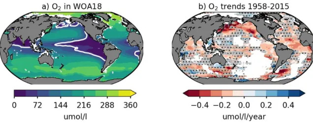
North and South tropical Pacific Ocean and the Northern Arabian Sea (Figure 1). In the eastern Tropical Atlantic, there are also well-studied OMZs, but these have relatively higher oxygen concentrations. Oxygen levels within the OMZ influence their biological and biogeochemical impacts: the transition to hypoxia (typically O2< 60 M) leads to a major loss of biodiversity
and mortality events for many macro-organisms [Vaquer-Sunyer and Duarte, 2008], suboxia (typically O2< 1-5 M) corresponds to the transition from O2-based respiration to nitrate-based
respiration and denitrification, and anoxia (typically O2< 0.1 M) corresponds to the transition
from nitrate-based respiration to sulfate reduction [Paulmier and Ruiz-Pino, 2009]. Note that the thresholds for these transitions vary in the literature and are given here as an indication.
Hypoxic conditions in the water column are usually associated with low ventilation and high oxygen demand. OMZs are hence found in the poorly ventilated shadow zones of the subtropical oceans, where subsurface streamlines recirculate beneath a shallow mixed-layer with essentially no direct advective connection to the surface ocean [Luyten et al., 1983]. In these domains, the residence time in the thermocline is at a maximum, and oxygen is slowly supplied mainly through mixing processes [Gnanadesikan et al., 2012]. Near the surface, these
regions are also biologically productive upwelling systems producing organic matter that fuels intense bacterial respiration when it sinks through the thermocline. The strong and localized subsurface biological oxygen consumption generates strong spatial gradients in oxygen at the edges of the shadow zones, making mixing all the more important to the oxygen balance in major OMZs. Understanding the processes and quantifying the rates of along-isopycnal and diapycnal mixing is therefore crucial for assessing oxygen budgets in the OMZs. The dominant role of mixing as a source of oxygen in the OMZs is illustrated by the few examples below.
The OMZs in the eastern tropical Atlantic are unique among the OMZs in that they are rarely suboxic, with minimum O2 concentrations typically above 40 M (Figure 1). The higher O2
levels, relative to OMZs in the Pacific Ocean, are likely the result of mixing with recently ventilated water masses. In the eastern tropical North Atlantic, just west of the coastal upwelling region offshore of Mauritania and Senegal, these water masses include the Labrador Sea Water and Mediterranean Overflow Water, which sit just beneath the oxygen minimum, and subtropical Central Waters found to the west [Brandt et al., 2010; 2015], and Subantarctic Mode Water and Antarctic Intermediate Water to the south. The rates of mixing in the eastern tropical North Atlantic OMZ, have been quantified from a number of studies, using independent methods [Banyte et al., 2012; 2013; Hahn et al., 2014; Rudnickas et al., 2019]. Mixing coefficients were recently evaluated from the dispersion of carefully-ballasted isopycnal RAFOS floats, which drifted passively on an isopycnal surface, recording their position 4 times a day via acoustic tracking [Rudnickas et al., 2019]. These floats were deployed in clusters at the core of the oxygen minimum (the 27.1 potential density surface, at about 500 m). Dispersion of the floats was used to estimate a coefficient of turbulent diffusivity, which grows with increasingly large spatial scales, plateauing at the mesoscale (nominally 100 km) at highly anisotropic values of 800 ± 310 m2 s-1 in the meridional direction and 1,410 ± 490 m2 s-1 in the
zonal direction.
The diffusivities diagnosed from the spreading of the isopycnal floats are consistent with those revealed from the spread of a patch of intentionally-released chemical tracer (CF3SF5) at
approximately 300 m over time [Banyte et al., 2012], which led to an estimate of isopycnal diffusivity of 500 m2 s-1 in the meridional direction and 1,200 m2 s-1 in the zonal direction
[Banyte et al., 2013]. Further, the vertical spreading of the chemical tracer allowed for the estimate of a diapycnal diffusivity coefficient of 10-5 m2 s-1. The anisotropy of the isopycnal
supports the idea that zonally-elongated mesoscale eddies [Rypina et al., 2012] play a major role in controlling mixing. It has also been suggested that the background potential vorticity (PV) distribution may shape the anisotropy by limiting mixing across PV contours [O'Dwyer
et al., 2000]. However, this hypothesis could not be confirmed in the eastern subtropical North
Atlantic near the OMZ, where surface drifters cross mean PV contours, resulting in a poor correlation between the orientations of the mean PV contours and the direction of spreading [Rypina et al., 2012].
The quantification of the isopycnal and diapycnal diffusivities provide valuable constraints on oxygen budgets of the OMZs, which must take into account biological sources and sinks, advection, and mixing of oxygen. Given the climatological O2 concentrations in the eastern
tropical North Atlantic OMZ and the observationally-constrained isopycnal and diapycnal diffusivity rates, it is possible to estimate the leading terms in the steady state oxygen budget in the eastern tropical North Atlantic OMZ [Brandt et al., 2015; Rudnickas et al., 2019]. Brandt et al. [2015] solved for these terms as the synthesis from a number of field programs and found that meridional mixing was the biggest supply term of oxygen at the core of the OMZ, balancing its removal via respiration (Figure 2). Vertical mixing (black) and zonal advective and diffusive transport (solved as a residual), appear to be smaller supply terms — each providing about 15% of the supply by meridional mixing. The residual transport term is the dominant O2
supply near the ocean’s surface, but it is much smaller than the isopycnal mixing supply at the depth of the oxygen minimum. Meridional mixing is the biggest supply term, despite the fact that the meridional diffusivity coefficient is about half of the zonal coefficient [Banyte et al., 2013; Rudnickas et al., 2019]. The reason is that meridional oxygen gradients are much stronger than zonal gradients (Figure 1a). Zonal jets are mainly responsible for maintaining these sharp meridional oxygen gradients, as they advect high-oxygen waters eastward near the equator [Brandt et al., 2015].
The role that each term plays in the oxygen budgets of OMZs can be further assessed by comparing model simulations at different resolutions. Increasing model resolution generally allows for improved large-scale circulation, and also for explicit representation of eddy mixing. In the equatorial Pacific OMZ, for example, the large-scale equatorial circulation tied to the Equatorial Under Current (EUC) supplies oxygen to the upper part of the OMZ (top 300 m), and eddy transport achieves the final supply to the OMZ [Busecke et al., 2019]. With a coarse resolution (1°) Earth System model, Busecke et al. [2019] noted an unrealistic deceleration of the EUC westward compared to observations (Figure 3 a-b, grey contour). As a result, the EUC
in this model leaked large amounts of oxygen in the central Pacific and the upper boundary of the OMZ was too deep (westward slanted upper boundary at 600 m in the central Pacific, Figure 3 a-b). In addition, the parameterized eddy transport used in this coarse resolution run remained confined to the edges of the OMZ (Figure 3 h). When the same model was run at finer resolution (1/10°), the EUC circulation and upper OMZ were more realistic (sustained eastward velocity across the basin and upper OMZ flat boundary at 300 m depth). Moreover, the presence of alternating equatorial zonal jets and intense eddy circulation in the fine resolution simulation enabled the presence of sharp meridional O2 gradients and the transport
by mixing of the oxygen carried by the EUC to the OMZ, reaching the OMZ core (defined here as O2< 40 M, Figure 3 i).
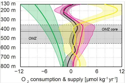
The important role that eddy-mixing plays in the oxygen balance was also established for the world’s thickest OMZ in the Arabian Sea. With a regional model of the North Indian Ocean whose horizontal grid size (1/12°) is fine enough to explicitly solve part of the mesoscale spectrum, Resplandy et al. [2012] have shown that mixing (which in their case included vertical diffusion and eddy advection) was the only oxygen source balancing the strong biological activity in the OMZ core (Figure 4). In their model, 90% of the O2 supply to the OMZ core
was from eddy mixing (46% from vertical eddy advection and 44% from horizontal eddy advection) and the other 10% from vertical diffusion. They also noted that, to a lesser extent, the mean large-scale advection actually removed O2 from the OMZ core in their budget (as was
also the case in the Pacific OMZ, Figures 4 c-d, 3 g).
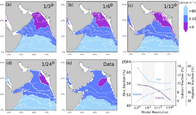
Lachkar et al. [2016] further examined the essential role of eddy mixing on the volume of the OMZ in a suite of regional model simulation of the Arabian Sea with increasing horizontal resolution. They noted that, as resolution increased from 1/3° to 1/24° and eddy mixing was better resolved, the volume occupied by suboxic waters (defined in their case as O2 < 4 M)
decreased by a factor close to two, in better agreement with observations (purple area in Figure 5). Their analysis revealed that underestimating eddy mixing, as was occurring in the coarser resolution runs, caused a strong overestimation of the volume of suboxic waters. However they also noted that eddy-driven ventilation (which provided an additional source of O2 at
subsurface) was partially offset by a biological feedback (which provided an additional sink of O2 at subsurface). At fine resolution, the smaller extent of suboxic waters reduced
denitrification (loss of nitrate due to microbial nitrate reduction in low O2 environment) thereby
respiration at subsurface. The consequence of this biological feedback was the increase of the volume of hypoxic waters (defined as 4 < O2< 60 M, blue area in Figure 5). Further, they
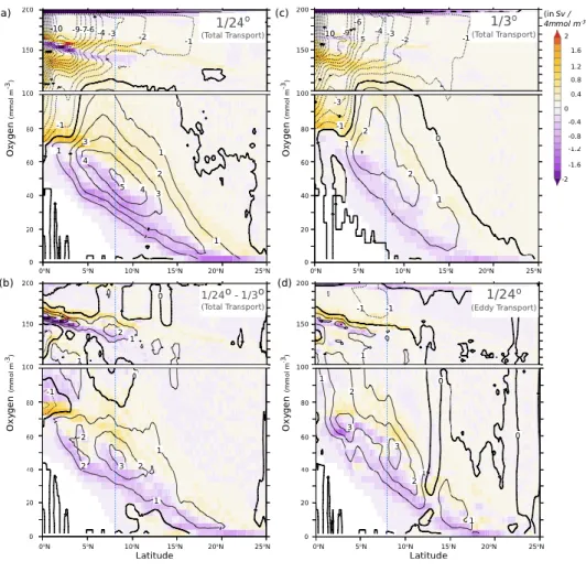
estimated the role of eddy mixing in the ventilation of the OMZ through the change in overturning circulation between their fine-resolution (1/24°) and coarse-resolution (1/3°) runs (Figure 6). Ventilation by highly oxygenated waters (O2 > 60 M, in yellow) was quantified in
terms of the volume of hypoxic water exported out of the Arabian Sea (O2 < 60 M, in purple).
The transport of these hypoxic waters out of the Arabian Sea increased from 2 to 5 Sv when the resolution increased from 1/3° to 1/24° (Figure 6 a-c). This additional transport was essentially due to the eddy mixing term at 1/24°, which explains most of the differences in transport between the 1/3° and 1/24° runs (Figure 6 b-d).
One of the great uncertainties in ESMs is how they parameterize lateral eddy mixing (Melet et al., this issue), and the degree to which these parameterizations, relative to the resolved circulation, hold the key to faithfully representing OMZs and accurately predicting their future change. Given that eddy mixing is the leading oxygen supply term to the OMZs [Gnanadesikan
et al., 2013] and also that narrow currents, which are often unresolved in climate models, play
a key role in setting the large-scale O2 gradients [Brandt et al., 2015; Lachkar et al., 2016;
Busecke et al., 2019; Rudnickas et al., 2019], it is not surprising that ESMs have difficulties in
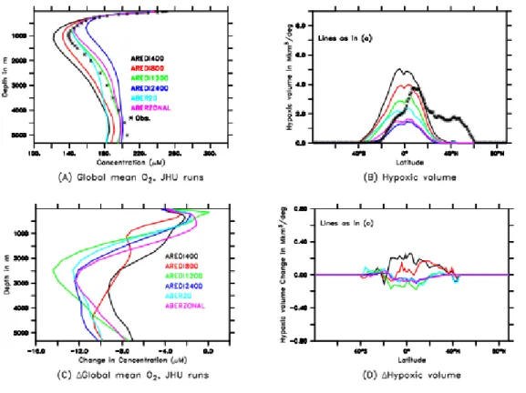
predicting the volume of OMZ [Bopp et al., 2013; Cabré et al., 2015; Bopp et al., 2017]. Gnanadesikan et al. [2013] and Bahl et al. [2019] have explored the sensitivity of the global volume of hypoxic waters (which they defined as O2< 88 M) simulated by an ESM to the
choice of the isopycnal mixing coefficient (AREDI) within the range of values used by the current
generation of ESMs. They found that low‐mixing models simulate larger volumes of hypoxic waters than high‐mixing models (Figure 7B). This result is in line with the results of Lachkar et al. [2016] of expanding suboxic waters, but, because denitrification is absent in the Bahl et al. [2019] model, it occurs without the feedback of slowed denitrification increasing primary productivity and the associated respiration [Lachkar et al., 2016]. The isopycnal mixing coefficient, AREDI, is typically held constant in ocean models and is often isotropic.
Gnanadesikan et al. [2013] and Bahl et al. [2019] have also attempted to use a more realistic, spatially-variable AREDI, with very large values at the edges of boundary currents and very low
values far from such currents, following Abernathey and Marshall [2013] (ABER2D, Figure 7), or more simple zonally averaged version of the ABER2D parameterization (ABERZONAL, Figure 7). These two experiments yielded similar results than those with a large, and constant,
parameterizations may represent eddy mixing too simplistically, or that the resolved circulation plays an important role that cannot be simply solved by improving the parametrization of lateral mixing.
2. Role of mixing on global deoxygenation
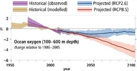
One of the most dramatic transformations of the global ocean over the past fifty years is its loss of oxygen (Figure 1b and Figure 8). The last Intergovernmental Panel on Climate Change Special Report on the Ocean and Cryosphere in a Changing Climate [IPCC, 2019] assessment reports that over this period, the upper 1000 m of the ocean has lost about 2% of its oxygen reservoir [Ito et al., 2017; Schmidtko et al., 2017]. Deoxygenation is projected to continue during the 21st century unless greenhouse gas emissions are rapidly curtailed, as in the RCP2.6
scenario (Figure 8) [Bopp et al., 2013; Cabré et al., 2015; Bopp et al., 2017; Hameau et al., 2020; Kwiatkowski, 2020; Li et al., 2020]. For marine animals living in oceanic environments just at the edge of their metabolic oxygen needs, the declining oxygen reservoir represents an immediate threat to survival [Vaquer-Sunyer and Duarte, 2008].
The drivers of deoxygenation remain poorly quantified [Oschlies et al., 2018]. The easiest to quantify is due to the reduced solubility of oxygen as the ocean warms. In addition, warming can reduce exchange between the surface and intermediate depths. Together, these changes slow the supply of oxygen to the ocean interior. On the other hand, declining exchange between the surface and subsurface also reduces the supply of nutrients to the euphotic layer, limits primary production, and diminishes the organic matter export that fuels oxygen consumption by respiration in the subsurface layers. Deoxygenation results from an imbalance between the decreased oxygen consumption and decreased oxygen supply. The fraction of total oxygen decline due to solubility (O2sat) can be evaluated from the changes in temperature and salinity
of the seawater, and 40-50% of the contemporary oxygen loss has been attributed to the solubility effect [Helm et al., 2011; Bopp et al., 2013; Schmidtko et al., 2017]. The remainder, Apparent Oxygen Utilization (-AOU= O2 - O2sat) represents the change in oxygen
Numerical models simulate a global average oxygen decline over the past several decades, but the multi-model average underestimates the rate of observed decline (Figure 8). The models also misrepresent the spatial distribution of oxygen decline, particularly in the tropics [Oschlies
et al., 2017]. ESMs project deoxygenation at the global scale of another 3.5-5.5% from the
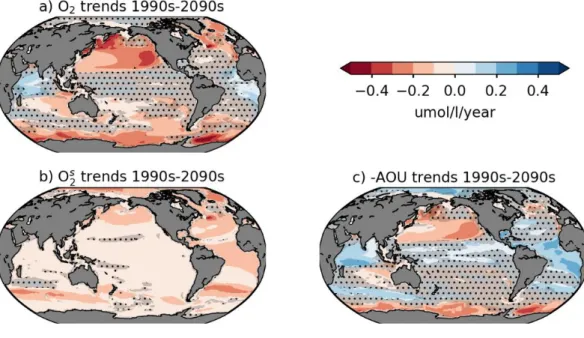
present to 2100 under the high-emissions scenario (RCP8.5), with stronger deoxygenation at mid- and high latitudes [Bopp et al., 2013; Cocco et al., 2013]. These projections disagree with one another on the sign of the trend in the tropical Oceans (i.e. in Figure 9a the gray stippled regions show where at least one of the models do not agree on the sign of the future change; see section 3 for discussion on OMZ response). At the global scale, ESMs project consistently reduced oxygen solubility tied to ocean warming at the global scale (O2sat, Figure 9b). This
solubility effect is reinforced by a strong reduction in oxygen supply by ventilation at mid- and high latitudes (-AOU, Figure 9c).
Assessing the drivers of deoxygenation quantitatively, and the uncertainties associated with each of them, is a necessary first step to understand the misfit between model and data, and the model spread. These drivers include changes in respiration, in ocean circulation, including the primarily wind-forced subtropical gyres, and/or changes in the overturning circulation that supplies oxygen-rich water to the deep ocean via convective mixing. The changing dynamics also encompasses smaller scale processes, like turbulent diapycnal and isopycnal mixing across oxygen gradients. In the following, we review two model studies that have attempted to tease apart the different factors involved in the change of AOU and have highlighted the leading role of mixing in the deoxygenation imbalance. Both studies arrive at similar conclusions about the importance of mixing in setting the pace of global deoxygenation in a warming world, using independent models and different methodologies.
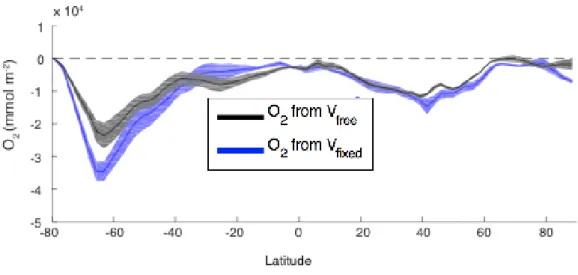
One study [Palter and Trossman, 2018] manipulated a model framework in order to fully separate the roles of changing large-scale ocean circulation from changes in mixing. In the first set of simulations (run in triplicate to reduce the impact of internal variability on the results), the atmospheric CO2 concentrations were increased at 1% per year, until they doubled at
approximately year 70, and all components of the climate system evolved freely in response to this perturbation (Vfree). The second set of simulations was identical, except that the ocean
velocity field was held fixed at its pre-industrial values (Vfixed). Thus, the role of parameterized
mixing versus resolved circulation is revealed from the difference between Vfree and Vfixed
could not be blamed for the loss of oxygen from the ocean. In fact, circulation changes slightly slowed the global deoxygenation rate, both by reducing the pace of warming and stabilizing mixed layer depths, particularly in the Southern Ocean (Figure 10) [Trossman et al., 2016]. In other words, in this model on multi-decadal time scales, changes in the parameterized mixing were responsible for essentially all of the deoxygenation not attributable to the effect of warming on oxygen solubility. Further, the reduction in the oxygen consumption through respiration provided only a minor offset (less than 5%) to counterbalance the much larger loss of oxygen supply to the ocean interior.
Confirming the first-order role of mixing as a cause of global deoxygenation, Couespel et al. [2019] examined the oxygen budget in an ESM forced by a high-CO2 emission scenario for the
21st century, using diagnostics of oxygen subduction. They partitioned physical dissolved oxygen exchanges between the surface and ocean interior into a component due to the kinematic flux linked to the subduction of water masses containing oxygen, and a diffusive flux due to oxygen mixing across the mixed-layer interface. For sake of simplicity, these terms were named « kinematic subduction » of oxygen and « diffusive subduction » of oxygen in Couespel et al. [2019], with the following definitions: the kinematic subduction of oxygen (Skin, equation 2) is the product of the kinematic subduction (S, equation 1), in volume flux per unit area, as defined by Cushman-Roisin [1987], by the oxygen concentration (equation 2); and the diffusive subduction of oxygen (Smix, equation 3) is defined as the transfer of oxygen by diffusion across
the mixed-layer interface.
Here, h is the mixed layer depth, u and w are the horizontal and vertical velocities at the base of the mixed layer, and kz and kl are the vertical and isopycnal mixing coefficients at that depth.
The kinematic flux (or “kinematic subduction”, equations 1 & 2) includes advection through vertical and horizontal currents, entrainment/detrainment caused by temporal changes of the
depth of the mixed-layer, as well as advection by bolus velocities used to parameterize the flattening of isopycnals by eddies [Gent and McWilliams, 1990].
The diffusive flux (or “diffusive subduction”, equation 3) includes both vertical mixing and isopycnal mixing by eddies, which are proportional to oxygen gradients at the base of the mixed-layer.
The changes between the beginning and the end of the 21st century reveal that, though kinematic
subduction locally shows the largest amplitude of changes, these changes swing between large increases and decreases, and therefore sum to a small global reduction in the subduction of oxygen (Figure 11). This balance is particularly apparent in the Southern Ocean, where the Skin
changes are mainly a response to the southward shift of the westerly winds. In contrast, diffusive subduction is projected to decrease more uniformly over the globe. Therefore, when globally integrated, negative changes in Smix sum to over 75% of the reduction in the total
subduction of O2 (small inset in Figure 11). Interestingly, the reduction in Smix was linked to a
reduction of the vertical oxygen gradient across the base of the surface mixed-layer rather than a reduction in mixing efficiency. The weakened vertical gradient can be explained by a reduction in oxygen undersaturation below the mixed layer, a direct consequence of the diminution in respiration following the reduction in nutrient supply by mixing and biological production at the surface. The globally-integrated decline in respiration (green bar in Figure 11 inset), which acts as a negative feedback on global deoxygenation, was much smaller than the decline in O2 supply by subduction (the sum of the red and cyan bars in Figure 11).
Regardless of the difference in methodologies, these two modeling studies come to similar conclusions about the drivers of global deoxygenation (Figures 10 and 11). Under strong warming scenarios, both project on the order of 50 Tmol y-1 of oxygen loss from the global
ocean, with the principal driver of this loss due to changes in mixing. Though these mixing changes are also accompanied by reduced global respiration in both models, this diminished sink term does not substantially offset the slowing O2 supply to the ocean interior (inset in
Figure 11). The spatial patterns in Figures 10 and 11 might be interpreted to suggest that these models — while having similar global rates and drivers of deoxygenation — are realizing the O2 losses in different regions. However, Figure 10 depicts the change in the
vertically-integrated O2 reservoir, while Figure 11 shows the change in the subduction flux of O2 across
the base of the mixed layer. The change in the O2 reservoir suggests that the largest losses will
agreement with the historical O2 trends in Figure 1 and ensemble-mean projected changes in
Figure 9.
3. Response of OMZ to global warming
A major concern is that OMZs may expand in the 21st century in response to ocean warning,
threatening the survival of marine organisms that rely on dissolved oxygen for respiration, and affecting the biogeochemical cycling of carbon and nitrogen, potentially amplifying global warming [Stramma et al., 2008; Keeling et al., 2010; Fu et al., 2018; Lachkar et al., 2018;
Resplandy, 2018; Lachkar et al., 2019]. Observations indicate strong regional variations in the
deoxygenation of the tropical oceans. OMZs have clearly expanded since the 1970s in the equatorial Pacific and Atlantic Oceans [Stramma et al., 2008; Brandt et al., 2010] but with strong multi-decadal temporal variations [Deutsch et al., 2014]. In the Arabian Sea, the northern and western pars of the OMZ are expanding, whereas the southern part is shrinking [Banse et
al., 2014; Piontkovski and Al-Oufi, 2014; Queste et al., 2018]. ESMs project dramatically
different changes in OMZ volume by 2100 (ranging from −2% to +16%) [Bopp et al., 2013;
Cabré et al., 2015]. Despite these differences, ESMs agree on many features that control
deoxygenation in tropical OMZs. The solubility effect in tropical OMZs is partly offset by an increased oxygen supply by ventilation and a reduced biological oxygen consumption [Cabré
et al., 2015; Bopp et al., 2017]. It has also been suggested that tropical OMZ might shrink after
2100 following their initial expansion [Fu et al., 2018]. The high uncertainties in OMZs evolution between ESMs largely arise from differences in the magnitude and timing of these ventilation and biological changes and how strongly they offset each other [Resplandy, 2018]. For instance, the Pacific OMZ is more sensitive to changes in equatorial circulation in models that underestimate eddy-driven O2 supply by mixing, which might explain the disparate future
deoxygenation responses across models in this region [Shigemitsu et al., 2017; Busecke et al., 2019].
ESMs frequently project increased ventilation in tropical OMZs in the future, with diapycnal and isopycnal mixing accelerating the renewal of OMZ waters [Gnanadesikan et al., 2007;
Bopp et al., 2017; Bahl et al., 2019]. Here we report on two modeling studies that have shown
value of the mixing coefficient, one study focused on diapycnal mixing [Duteil and Oschlies, 2011], the other on isopycnal mixing [Bahl et al., 2019].
Bahl et al. [2019] varied the isopycnal mixing coefficient within the range used by current ESMs (constant coefficients from 400 to 2400 m2s-1, and two spatially variable coefficients
with local values up to 10 000 m2s-1 in high-mixing areas). Under doubled atmospheric CO2,
the volume of hypoxic waters increased in models with low-mixing but decreased in models with high-mixing and with spatially-variable mixing coefficients (Figure 7d). Surprisingly, these changes in hypoxic volume (largest increase in hypoxic volume in low-mixing models, Figure 7d) were decoupled from the total amount of deoxygenation (largest decline in oxygen in high-mixing models, Figure 7c).
Duteil and Oschlies [2011] varied the background value of vertical diffusivities within a range corresponding to observed values and to values currently used in ocean models (from 0.01 to 0.5 cm2 cm2s-1) in a coarse-resolution ESM in which diapycnal mixing was parameterized as
the sum of the regionally heterogeneous tidal and homogenous background vertical mixing. Under projected 21st century CO2 emissions, all of their model experiments predicted global
deoxygenation, but the extent of suboxia (which they defined as O2 < 5 M) expanded only for
mixing rates higher than 0.2 cm2s-1, and declined for lower mixing rates (by up to +/- 40% by
2100). In their experiments, both respiration and ventilation decreased with global warming. But when the vertical mixing coefficient exceeded 0.2 cm2s-1, the relative decline in respiration
was smaller than the decline in physical supplies of oxygen, resulting in an expansion of the suboxic volume; in contrast at lower mixing intensities, the relative decline in respiration was larger than the decline in physical supplies, resulting in a reduction of the suboxic volume.
These two studies both report a non-monotonic response of the volume of suboxic and hypoxic waters to global warming against mixing coefficients, which reflects the fact that mixing affects the OMZ directly via ventilation and indirectly via biological feedbacks (respiration and denitrification).
In Figure 12, we have attempted to conceptualize the possible responses of OMZs to global warming. The outcome for the OMZ depends on the balance between reduced oxygen supply (due to reduced mixing) and reduced oxygen consumption (due to reduced respiration). The respective changes in ventilation and respiration depend on multiple factors, such as the nutrient and oxygen gradients, the contribution of mixing to total transport for nutrient and oxygen, and
the removal of nutrients by denitrification. Moreover the changes due to mixing add to other responses to climate change, such as changes in large-scale advection of oxygen and of nutrients. Finally, the sign of the change in mixing intensity itself is highly uncertain and region dependent [Gnanadesikan et al., 2007; Bopp et al., 2017; Bahl et al., 2019]. This schematic shows how the OMZ can globally expand or shrink, but the outcome can also be different at the top and bottom of the OMZ, causing it to either deepen or get closer to the surface.
Conclusions and Grand Challenges
We have reviewed current knowledge on the role of mixing on the oxygen budget in the ocean, and its imbalance driven by climate change. The pace of global deoxygenation, as well as the volume and intensity of OMZs and their projected changes have been shown to be particularly sensitive to lateral and diapycnal mixing. Mixing directly influences ocean ventilation but also indirectly influences oxygen via biological feedbacks (respiration and denitrification). Weaker mixing associated with global warming can reduce the supply of oxygen to the ocean interior while simultaneously slowing the upward transport of nutrients that sustains biological production in the upper ocean and the consumption of that organic matter via microbial respiration at depth. The traditional view is that the effect of reduced ventilation is partly offset by this slowdown in biological respiration at depth. Yet, the net effect of the reduced ventilation and respiration induced by mixing strongly varies in space and probably in time depending on oxygen levels and mixing rates. In ventilation regions at mid- and high latitudes, the decline in respiration is strongest near the surface, which can reduce the vertical oxygen gradient, thereby slowing the downward mixing of oxygen at the base of the mixed layer, and counter intuitively, reinforce the effect of deoxygenation through reduced ventilation [Couespel et al., 2019]. In OMZs, where mixing rates are low, the supply and utilization of oxygen are tightly coupled. As a result, the respiration changes can counterbalance and even exceed mixing-induced changes in ventilation [Duteil and Oschlies, 2011; Fu et al., 2018; Bahl et al., 2019]. In addition, the respiration feedback in OMZs is reinforced by changes in microbial metabolic pathways between oxygen-based and nitrate-based (denitrification) respiration, stabilizing oxygen levels and OMZs volume [Lachkar et al., 2016]. Uncertainties in this subtle balance between mixing-induced ventilation and the associated biological feedbacks contribute to the strong bias in present simulated OMZ volume and to uncertainties in their future evolution [Resplandy, 2018].
Current ESMs often misrepresent observed oxygen patterns and, on average, underestimate historical deoxygenation. There are three main potential causes for these misrepresentations [Oschlies et al., 2017]: unaccounted variations in respiratory oxygen demand, missing biogeochemical feedbacks, and/or unresolved transport processes. The reasons that a model misrepresents the spatial patterns of ocean oxygen, particularly the size and O2 concentrations
in OMZs, may be distinct from the causes of the mismatch in globally-averaged rates of deoxygenation.
The studies reviewed herein provide evidence that (sub-)mesoscale eddies strongly influence the volume of the lowest-oxygen water in the global OMZs. Therefore, the parameterized representation of these eddies in coarse-resolution ESMs is critical to accurately simulate these regions and their evolution in the future. Current eddy mixing parameterizations rely on a diffusivity operator that acts on lateral oxygen gradients. Deoxygenation rates and the volume of OMZs are very sensitive to the value of the diffusivity coefficients of this operator, and neither varying this diffusivity across a wide range of constant values, nor representing its spatial variability [Abernathey and Marshall, 2013] was sufficient to bring the volume of hypoxic water simulated by a coarse resolution ESM in full agreement with observations [Gnanadesikan et al., 2013; Bahl et al., 2019]. On the other hand, regional models show a significant improvement in their representation of OMZs when the grid resolution is increased [Lachkar et al., 2016; Busecke et al., 2019]. Importantly, increasing grid resolution not only allows the model to explicitly resolve eddy-driven mixing but also improves the large-scale circulation [Lévy et al., 2010; Busecke et al., 2019], and both aspects matter to the ventilation of the OMZ [Brandt et al., 2010; Resplandy et al., 2012; Rudnickas et al., 2019]. Mixing depends not only on mixing strength but also on oxygen gradients. Any factor that contributes to setting this gradient, such as the respiratory oxygen consumption or the large scale circulation, may lead to a misrepresentation, or improvement, in the mixing transport of oxygen. Finally, some important biogeochemical feedbacks, such as the switch from aerobic respiration to denitrification, depend on the strength of mixing [Lachkar et al., 2016]. Therefore, the three different causes for oxygen misrepresentation interact nonlinearly, with the biogeochemical feedback being constrained by the amount of oxygen supplied by mixing, which itself is influenced by the biological oxygen demand.
In addition to playing a central role in the intensity and volume of OMZs, mixing also strongly influences the rate of global deoxygenation. Higher isopycnal diffusivity, or diffusivities that
vary spatially, can change the total deoxygenation in response to warming by up to 50%. This sensitivity points to isopycnal mixing as an under constrained parameterized process with high leverage to influence the deoxygenation [Bahl et al., 2019; Jones and Abernathey, 2019]. Likewise, changes in diapycnal mixing can exert a strong influence on global oxygen levels, with the role of mixing across the base of the mixed layer, termed diffusive subduction [Couespel et al., 2019], contributing a large share to global average deoxygenation. Mixing appears to be a particularly strong driver when deep convection slows at high latitudes, denying the densest layers of the ocean interaction with the atmosphere [Palter and Trossman, 2018].
Given the threat posed to ocean ecosystems by deoxygenation, improving the parameterization of mixing in climate models is critical to reliably project future changes in oceanic oxygen distribution.
Acknowledgments. We are grateful to Peter Brandt, Julius Busecke and Anand Gnanadesikan
who kindly shared with us or adapted figures from some of their previous work, and to Alessandro Tagliabue who adapted a figure from the IPCC-SROC SPM report. We also thank Jan Zika and Ric Williams who provided insightful reviews that helped to improve this chapter. This work was supported by ANR SOBUMS (ANR-16-CE01-0014). ZL and ML received support from New York University Abu Dhabi Institute's Center for Prototype Climate Modeling. LR gratefully acknowledges support of the High Meadows Environmental Institute "Climate and Energy Grand Challenge" and "Carbon Mitigation Initiative” and the Sloan Foundation Research Fellowship. JBP was supported by NSF-1736985.
References
Abernathey, R. P., and J. Marshall (2013), Global surface eddy diffusivities derived from satellite altimetry, J. Geophys. Res. Ocean, 118(2), 901–916, doi:10.1002/jgrc.20066. Babbin, A. R., D. Bianchi, A. Jayakumar, and B. B. Ward (2015), Rapid nitrous oxide cycling
in the suboxic ocean, Science, 348(6239), 1127–1129, doi:10.1126/science.aaa8380. Bahl, A., A. Gnanadesikan, and M. A. Pradal (2019), Variations in Ocean Deoxygenation
Across Earth System Models: Isolating the Role of Parameterized Lateral Mixing, Glob.
Biogeochem. Cyc., 33(6), 703–724, doi:10.1029/2018GB006121.
minimum zone of the open Arabian Sea: variability of oxygen and nitrite from daily to decadal timescales, Biogeosciences, 11(8), 2237–2261, doi:10.5194/bg-11-2237-2014-supplement.
Banyte, D., M. Visbeck, T. Tanhua, T. Fischer, G. Krahmann, and J. Karstensen (2013), Lateral diffusivity from tracer release experiments in the tropical North Atlantic thermocline, J. Geophys. Res. Ocean, 118(5), 2719–2733, doi:10.1002/jgrc.20211. Banyte, D., T. Tanhua, M. Visbeck, D. W. R. Wallace, J. Karstensen, G. Krahmann, A.
Schneider, L. Stramma, and M. Dengler (2012), Diapycnal diffusivity at the upper boundary of the tropical North Atlantic oxygen minimum zone, J. Geophys. Res. Ocean,
117(C9), doi:10.1029/2011JC007762.
Bianchi, D., J. P. Dunne, J. L. Sarmiento, and E. D. Galbraith (2012), Data-based estimates of suboxia, denitrification, and N2O production in the ocean and their sensitivities to
dissolved O2, Glob. Biogeochem. Cyc., 26(2), doi:10.1029/2011GB004209.
Bopp, L. et al. (2013), Multiple stressors of ocean ecosystems in the 21st century: projections with CMIP5 models, Biogeosciences, 10(10), 6225–6245, doi:10.5194/bg-10-6225-2013. Bopp, L., L. Resplandy, A. Untersee, P. Le Mezo, and M. Kageyama (2017), Ocean
(de)oxygenation from the Last Glacial Maximum to the twenty-first century: insights from Earth System models, Philosophical Transactions of the Royal Society A:
Mathematical, Physical and Engineering Sciences, 375(2102), 20160323,
doi:10.1098/rsta.2016.0323.
Brandt, P. et al. (2015), On the role of circulation and mixing in the ventilation of oxygen minimum zones with a focus on the eastern tropical North Atlantic, Biogeosciences,
12(2), 489–512, doi:10.5194/bg-12-489-2015.
Brandt, P., V. Hormann, A. Kortzinger, M. Visbeck, G. Krahmann, L. Stramma, R. Lumpkin, and C. Schmid (2010), Changes in the Ventilation of the Oxygen Minimum Zone of the Tropical North Atlantic, J. Phys. Oceanogr., 40(8), 1784–1801,
doi:10.1175/2010JPO4301.1.
Busecke, J. J. M., L. Resplandy, and J. P. Dunne (2019), The Equatorial Undercurrent and the Oxygen Minimum Zone in the Pacific, Geophys. Res. Lett., 46(12), 6716–6725,
doi:10.1029/2019GL082692.
Cabré, A., I. Marinov, R. Bernardello, and D. Bianchi (2015), Oxygen minimum zones in the tropical Pacific across CMIP5 models: mean state differences and climate change trends,
Biogeosciences, 12(18), 5429–5454, doi:10.5194/bg-12-5429-2015.
Cocco, V. et al. (2013), Oxygen and indicators of stress for marine life in multi-model global warming projections, Biogeosciences, 10(3), 1849–1868, doi:10.5194/bg-10-1849-2013. Couespel, D., M. Levy, and L. Bopp (2019), Major Contribution of Reduced Upper Ocean
Oxygen Mixing to Global Ocean Deoxygenation in an Earth System Model, Geophys.
Res. Lett., 46(21), 12239–12249, doi:10.1029/2019GL084162.
Cushman-Roisin, B. (1987), Subduction. Dynamics of the Oceanic Surface Mixed Layer, edited by P. Muller and D. Henderson, Hawaii Institute of Geophysics Special
Publication, 182–195.
Deutsch, C. et al. (2014), Centennial changes in North Pacific anoxia linked to tropical trade winds, Science, 345(6197), 665.
Dufour, C. O. et al. (2015), Role of Mesoscale Eddies in Cross-Frontal Transport of Heat and Biogeochemical Tracers in the Southern Ocean, J. Phys. Oceanogr., 45(12), 3057–3081, doi:10.1175/JPO-D-14-0240.1.
Duteil, O., and A. Oschlies (2011), Sensitivity of simulated extent and future evolution of marine suboxia to mixing intensity, Geophys. Res. Lett., 38(6), n/a–n/a,
doi:10.1029/2011GL046877.
Fu, W., F. Primeau, J. Keith Moore, K. Lindsay, and J. T. Randerson (2018), Reversal of Increasing Tropical Ocean Hypoxia Trends With Sustained Climate Warming, Glob.
Biogeochem. Cyc., 32(4), 551–564, doi:10.1002/2017GB005788.
Gent, P. R., and J. C. McWilliams (1990), Isopycnal mixing in ocean circulation models, J.
Phys. Oceanogr., 20, 150–155.
Gnanadesikan, A., D. Bianchi, and M.-A. Pradal (2013), Critical role for mesoscale eddy diffusion in supplying oxygen to hypoxic ocean waters, Geophys. Res. Lett., 40(19), 5194–5198, doi:10.1002/grl.50998.
Gnanadesikan, A., J. L. Russell, and F. Zeng (2007), How does ocean ventilation change under global warming? Ocean Science, 3(1), 43–53.
Gnanadesikan, A., J. P. Dunne, and J. John (2012), Understanding why the volume of suboxic waters does not increase over centuries of global warming in an Earth System Model,
Biogeosciences, 9(3), 1159–1172, doi:10.5194/bg-9-1159-2012.
Hahn, J., P. Brandt, R. J. Greatbatch, G. Krahmann, and A. Körtzinger (2014), Oxygen variance and meridional oxygen supply in the Tropical North East Atlantic oxygen minimum zone, Clim Dyn, 43(11), 2999–3024, doi:10.1007/s00382-014-2065-0. Hameau, A., T. L. Frölicher, J. Mignot, and F. Joos (2020), Is deoxygenation detectable
before warming in the thermocline? Biogeosciences, 17(7), 1877–1895, doi:10.5194/bg-17-1877-2020.
Helm, K. P., N. L. Bindoff, and J. A. Church (2011), Observed decreases in oxygen content of the global ocean, Geophys. Res. Lett., 38(23), n/a–n/a, doi:10.1029/2011GL049513. IPCC (2019), SROCC Summary for Policymakers, in IPCC Special Report on the Ocean and
Cryosphere in a Changing Climate, edited by H. O. Portner et al., pp. 1–36.
Ito, T., and C. Deutsch (2010), A conceptual model for the temporal spectrum of oceanic oxygen variability, Geophys. Res. Lett., 37(3), n/a–n/a, doi:10.1029/2009GL041595. Ito, T., S. Minobe, M. C. Long, and C. Deutsch (2017), Upper ocean O2 trends: 1958-2015,
Geophys. Res. Lett., 44(9), 4214–4223, doi:10.1002/2017GL073613.
Baxter.
Johnson, G. C., B. M. Sloyan, W. S. Kessler, and K. E. McTaggart (2002), Direct
measurements of upper ocean currents and water properties across the tropical Pacific during the 1990s, Prog. Oceanogr., 52(1), 31–61.
Jones, C. S., and R. P. Abernathey (2019), Isopycnal Mixing Controls Deep Ocean Ventilation, Geophys. Res. Lett., 46(22), 13144–13151, doi:10.1029/2019GL085208. Keeling, R. F., A. Kortzinger, and N. Gruber (2010), Ocean Deoxygenation in a Warming
World, Annu. Rev. Marine. Sci., 2(1), 199–229, doi:10.1146/annurev.marine.010908.163855.
Kwiatkowski, L. (2020), Twenty-first century ocean warming, acidification, deoxygenation, and upper ocean nutrient decline from CMIP6 model projections, Biogeosciences
Discuss., 1–43, doi:10.5194/bg-2020-16.
Lachkar, Z., M. Levy, and S. Smith (2018), Intensification and deepening of the Arabian Sea oxygen minimum zone in response to increase in Indian monsoon wind intensity,
Biogeosciences, 15(1), 159–186, doi:10.5194/bg-15-159-2018.
Lachkar, Z., M. Lévy, and K. S. Smith (2019), Strong Intensification of the Arabian Sea Oxygen Minimum Zone in Response to Arabian Gulf Warming, Geophys. Res. Lett.,
46(10), 5420–5429, doi:10.1029/2018GL081631.
Lachkar, Z., S. Smith, M. Levy, and O. Pauluis (2016), Eddies reduce denitrification and compress habitats in the Arabian Sea, Geophys. Res. Lett., 43(17), 1–9,
doi:10.1002/2016GL069876.
Lam, P., M. M. Jensen, A. Kock, K. A. Lettmann, Y. Plancherel, G. Lavik, H. W. Bange, and M. M. M. Kuypers (2011), Origin and fate of the secondary nitrite maximum in the Arabian Sea, Biogeosciences, 8(6), 1565–1577, doi:10.5194/bg-8-1565-2011.
Letscher, R. T., F. Primeau, and J. K. Moore (2016), Nutrient budgets in the subtropical ocean gyres dominated by lateral transport, Nature Geoscience, 9(11), 815–819,
doi:10.1038/ngeo2812.
Lévy, M., D. Iovino, L. Resplandy, P. Klein, G. Madec, A. M. Tréguier, S. Masson, and K. Takahashi (2012), Large-scale impacts of submesoscale dynamics on phytoplankton: Local and remote effects, Ocean Modelling, 43-44(C), 77–93,
doi:10.1016/j.ocemod.2011.12.003.
Lévy, M., P. Klein, A. M. Tréguier, D. Iovino, G. Madec, S. Masson, and K. Takahashi (2010), Modifications of gyre circulation by sub-mesoscale physics, Ocean Modelling,
34(1-2), 1–15, doi:10.1016/j.ocemod.2010.04.001.
Li, C., J. Huang, L. Ding, X. Liu, H. Yu, and J. Huang (2020), Increasing escape of oxygen from oceans under climate change, Geophys. Res. Lett., 1–13,
doi:10.1029/2019GL086345.
Luyten, J., J. Pedlosky, and H. Stommel (1983), Climatic inferences from the ventilated thermocline, Climatic Change, 5(2), 183–191, doi:10.1007/BF00141269.
O'Dwyer, J., R. G. Williams, J. LaCasce, and K. G. Speer (2000), Does the potential vorticity distribution constrain the spreading of floats in the North Atlantic? Journal Of Climate,
30(4), 721–732.
Oschlies, A., O. Duteil, J. Getzlaff, W. Koeve, A. Landolfi, and S. Schmidtko (2017), Patterns of deoxygenation: sensitivity to natural and anthropogenic drivers, Philosophical
Transactions of the Royal Society A: Mathematical, Physical and Engineering Sciences, 375(2102), 20160325, doi:10.1098/rsta.2016.0325.
Oschlies, A., P. Brandt, L. Stramma, and S. Schmidtko (2018), Drivers and mechanisms of ocean deoxygenation, Nature Geoscience, 11(7), 1–7, doi:10.1038/s41561-018-0152-2. Palter, J. B., and D. S. Trossman (2018), The Sensitivity of Future Ocean Oxygen to Changes
in Ocean Circulation, Glob. Biogeochem. Cyc., 32(5), 738–751, doi:10.1002/2017GB005777.
Paulmier, A., and D. Ruiz-Pino (2009), Oxygen minimum zones (OMZs) in the modern ocean, Prog. Oceanogr., 80(3-4), 113–128, doi:10.1016/j.pocean.2008.08.001. Piontkovski, S. A., and H. S. Al-Oufi (2014), The Omani shelf hypoxia and the warming
Arabian Sea, International Journal of Environmental Studies, 72(2), 256–264, doi:10.1080/00207233.2015.1012361.
Queste, B. Y., C. Vic, K. J. Heywood, and S. A. Piontkovski (2018), Physical controls on oxygen distribution and denitrification potential in the north west Arabian Sea, Geophys.
Res. Lett., 1–11, doi:10.1029/2017GL076666.
Resplandy, L. (2018), Will ocean zones with low oxygen levels expand or shrink? Nature,
557(7705), 314–315, doi:10.1038/d41586-018-05034-y.
Resplandy, L., M. Lévy, L. Bopp, V. Echevin, S. Pous, V. V. S. S. Sarma, and D. Kumar (2012), Controlling factors of the oxygen balance in the Arabian Sea's OMZ,
Biogeosciences, 9(12), 5095–5109, doi:10.5194/bg-9-5095-2012.
Rudnickas, D., Jr., J. Palter, D. Hebert, and H. T. Rossby (2019), Isopycnal Mixing in the North Atlantic Oxygen Minimum Zone Revealed by RAFOS Floats, J. Geophys. Res.
Ocean, 124(9), 6478–6497, doi:10.1029/2019JC015148.
Rypina, I. I., I. Kamenkovich, P. Berloff, and L. J. Pratt (2012), Eddy-Induced Particle Dispersion in the Near-Surface North Atlantic, J. Phys. Oceanogr., 42(12), 2206–2228, doi:10.1175/JPO-D-11-0191.1.
Schmidtko, S., L. Stramma, and M. Visbeck (2017), Decline in global oceanic oxygen content during the past five decades, Nature, 542(7641), 335–339, doi:10.1038/nature21399. Shigemitsu, M., A. Yamamoto, A. Oka, and Y. Yamanaka (2017), One possible uncertainty in
CMIP5 projections of low-oxygen water volume in the Eastern Tropical Pacific, Glob.
Biogeochem. Cyc., 31(5), 804–820, doi:10.1002/2016GB005447.
Spall, M. A., P. L. Richardson, and J. F. Price (1993), Advection and eddy mixing in the Mediterranean salt tongue, Journal of Marine Research, 51(4), 797–818.
Stramma, L., G. C. Johnson, J. Sprintall, and V. Mohrholz (2008), Expanding Oxygen-Minimum Zones in the Tropical Oceans, Science, 320(5876), 655–658,
doi:10.1126/science.1153847.
Trossman, D. S., J. B. Palter, T. M. Merlis, Y. Huang, and Y. Xia (2016), Large-scale ocean circulation-cloud interactions reduce the pace of transient climate change, Geophys. Res.
Lett., 43(8), 3935–3943, doi:10.1002/2016GL067931.
Vaquer-Sunyer, R., and C. M. Duarte (2008), Thresholds of hypoxia for marine biodiversity,
Proc. Nat. Ac. Sc., 105(40), 15452–15457.
Yamamoto, A., J. B. Palter, C. O. Dufour, S. M. Griffies, D. Bianchi, M. Claret, J. P. Dunne, I. Frenger, and E. D. Galbraith (2018), Roles of the Ocean Mesoscale in the Horizontal Supply of Mass, Heat, Carbon, and Nutrients to the Northern Hemisphere Subtropical Gyres, J. Geophys. Res. Ocean, 123(10), 7016–7036, doi:10.1029/2018JC013969. Yang, S. et al. (2020), Global reconstruction reduces the uncertainty of oceanic nitrous oxide
Figures
Figure 1: OMZs and deoxygenation. a) Climatological mean dissolved oxygen concentrations between 200m and 600m (data from Word Ocean Atlas, 2018). The 60 M contour is shown in white, and marks the boundary of major OMZs, which are located in the eastern North and South tropical Pacific Ocean, the Northern Arabian Sea and eastern tropical Atlantic. b) Observed 200-600 m oxygen trend between 1958 and 2015 (data from Ito et al. [2017]). Red colors indicate deoxygenation. The trend is computed by linear regression; white regions are those where less than 10 years of data were available; regions where trends are not significantly different from zero at the 80% confidence level (p_values > 0.2) are hatched in grey.
Figure 2: Tropical North Atlantic OMZ budget. Oxygen budget of the eastern tropical North Atlantic OMZ, derived from an extended observational program. Isopycnal meridional oxygen mixing (purple), vertical mixing (black), oxygen biological consumption (green), residual transport (the sum of zonal and meridional advection and zonal mixing, in yellow). The residual term is believed to be dominated by zonal advection, given evidence of narrow zonal jets providing oxygenated waters to the modeled region of the OMZ. All error estimates (coloured shadings) are the 95 % confidence (except the isopycnal meridional eddy supply, where the error was estimated from both the error of the oxygen curvature (95% confidence) and the error of the eddy diffusivity, where a factor 2 was assumed. Meridional mixing is the strongest O2
source in the core of the OMZ. The OMZ (between 350 and 550 m) is highlighted with grey shading, and its core (located at 420 m) is indicated by the black horizontal line. Adapted with permission from Brandt et al. [2015].
Figure 3: Pacific Ocean OMZ along the equator. Oxygen concentration (color) and Equatorial Undercurrent (EUC) zonal velocities (20, 60, 70, and 80 cm s-1 in gray contours)
from: (a) observations ([Bianchi et al., 2012] for O2 and [Johnson et al., 2002] for velocities),
(b) coarse 1° model (GFDL-CM1deg) and (c) eddying 1/10° model (GFDL-CM2.6). Oxygen budget associated with (d,e) biological activity, (f,g) large scale advection, and (h,i) mixing (vertical diffusion, eddy mixing and eddy advection - resolved at 1/10° and parameterized at 1°). Thick black lines indicate O2 contours of 80 M and 40 M. Fields are averaged between
Figure 4: The Arabian Sea OMZ budget. Oxygen budget between 200 and 1500 m in the Arabian Sea OMZ, simulated with a forced eddy-resolving ocean regional model [M/month]. a) Equilibrated dissolved oxygen distribution, averaged between 200 and 1500 m. The 30 M isoline delimits the OMZ. The oxygen tendency terms due to: b) vertical diffusion, c) mean horizontal advection, d) mean vertical advection, e) horizontal eddy advection, and f) vertical eddy advection. Only trends in the OMZ are shown. Mixing terms (vertical diffusion and eddy advection) are a source of dissolved oxygen to the OMZ (46% of the O2 supply over the OMZ
is from vertical eddy advection, 44% from horizontal eddy advection, 10% from vertical diffusion), while advective terms act on average as a sink (14% of O2 removal are by mean
vertical advection, 4% by mean horizontal advection, the remaining 82% by biological activity). Adapted from Resplandy et al. [2012].
Figure 5: The Arabian Sea OMZ sensitivity to model resolution. Horizontal distribution of dissolved oxygen at 250 m depth in winter (December–February) and volume fraction of the Arabian Sea OMZ (defined as the volume of suboxic waters, in purple) in a series of regional model experiments run at increasing horizontal grid resolution at (a) 1/3°, (b) 1/6°, (c) 1/12°, (d) 1/24°, and (e) from World Ocean Atlas 2009 data set. (f) Oxic (02 > 60 M), suboxic (O2 <
4 M), and hypoxic (4 < O2 < 60 M) volume fractions as simulated at different resolutions in
the top 1000 m. Increased model resolution reduces the volume of suboxic waters, but due to a biological feedback through reduced denitrification, it expands the volume of hypoxic waters and thus compresses habitats (i.e. compresses the volume of oxic waters). Reproduced from Lachkar et al. [2016].
Figure 6: The Arabian Sea OMZ eddy ventilation. Arabian Sea Meridional Stream Function in dissolved oxygen coordinates for the model experiments shown in Figure 5 (in Sv). (a) The 1/24° simulation, (b) the 1/3° simulation, (c) the difference between 1/24° and 1/3° simulations, and (d) the eddy component of the transport in the 1/24° simulation. Contour lines indicate the meridional stream function (positive indicates clockwise circulation). The color shading shows the meridional component of the transport. The vertical blue dashed line indicates the latitude of the southern tip of India. Similarities of the MSF between panels b) and c) highlights the central role of eddy mixing in the compression of the OMZ as grid resolution is increased. Reproduced from Lachkar et al. [2016].
Figure 7: Global oxygen reservoir sensitivity to lateral diffusivity coefficient, AREDI. A)
Global mean oxygen concentration profile during the preindustrial period in data (crosses) and a suite of the ESM2Mc ESM with different isopycnal mixing coefficients AREDI (color lines). In
ABER2D and ABERZONAL, a spatially variable AREDI was used, with relatively large values
of AREDI. B) Volume of hypoxic waters (defined as O2< 88 M). This panel highlights the
critical role of the strength of eddy mixing in controlling the volume of OMZs. The volume is larger when lateral diffusivity is smaller. C) Changes in total oxygen concentration under doubled CO2. Deoxygenation is larger when lateral diffusivity is larger. D: change in the
hypoxic volume under doubled CO2. The volume of hypoxic waters is increased for the smaller
values of AREDI (400 and 800 m2 s-1) and is decreased for all other cases. JHU = Johns Hopkins
Figure 8: Historical and projected global deoxygenation. Observed (purple) and modeled (brown) historical changes in the ocean since 1950, and projected future changes under low (blue, RCP2.6) and high (red, RCP8.5) greenhouse gas emissions scenarios, of the global mean ocean oxygen content between 100 and 600 m. Assessed observational trends span 1970–2010 centered on 1996. The shading represents one standard deviation across models. Adapted from
Figure 9: Projected deoxygenation trends. Deoxygenation trends between 200 and 600 m under RCP8.5 in the mean of nine simulations from different models of the CMIP5 framework in 2090-2099 relative to 1990-1999, for dissolved a) O2, b) O2sat and c) AOU. The trend is
computed as the mean of the last decade minus the mean of the first decade. Gray stippling marks low robustness between simulations (disagreement on sign of changes for more than one of the nine simulations).
Figure 10: Zonally averaged deoxygenation: role of advection and mixing on O2 content.
Zonally averaged deoxygenation under a doubling of atmospheric CO2 simulated with the
Geophysical Fluid Dynamics Laboratory Climate Model version 2 (CM2.1) at coarse resolution (CM2Mc). Each curve represents a mean over an ensemble of 3 simulations. In the Vfree set of
experiments, changes in both advection and changes in mixing are accounted for. In Vfixed, only
changes in mixing are accounted for. Comparison between the two sets reveals that the O2 decline is due largely to changes in mixing, while changes in circulation slightly slow the deoxygenation, particularly in the Southern Ocean where the oxygen loss is the most pronounced. Reproduced from Palter and Trossman [2018].
Figure 11: Zonally integrated deoxygenation: role of advection, mixing and respiration on O2 fluxes. Zonal integral of the projected change in kinematic oxygen subduction across the
surface mixed-layer (blue curve), of the projected change in oxygen mixing across the surface mixed-layer (red curve, diffusive subduction), of the projected change in respiration below the surface mixed-layer (green curve), and their sum (total) along the 21st century, in the IPSL RCP
8.5 CMIP5 simulations. Shown are cumulated fluxes over 110 years (1990 to 2099), and correspond to an average O2 loss of 55 TM y-1. Locally, projected changes in kinematic
subduction prevail, particularly in the Southern ocean. However when integrated globally (shown in small inset), global deoxygenation (total) is explained largely by a reduction in diffusive subduction (mixing), accompanied by a reduction in kinematic subduction, and partially offset by a reduction in respiration. Note that a zonal integral is shown here, and a zonal average is shown in Figure 10. Adapted from Couespel et al. [2019].
Figure 12: Possible responses of OMZs to reduced mixing associated with global warming. In this schematic representation of an OMZ, oxygen is replenished through physical processes (with intensity proportional to the light-blue circle, labelled “Ventilation”), a combination of advective (white arrows), and mixing (white swirls) processes. Nutrients are brought to the surface through upwelling (purple arrows) and vertical mixing (purple swirls). The intensity of photosynthesis depends on the intensity of the physical supply of nutrients through upwelling and mixing. For simplicity we neglect denitrification here, so the magnitude of photosynthesis equals that of respiration in all panels (the photosynthesis and respiration circles have identical sizes).a) The balanced state of an OMZ in which oxygen consumed by biological respiration is replenished through the ventilation of the ocean interior (the respiration and ventilation circles have identical sizes). In b) and c), mixing is assumed to be reduced in response to global warming but with opposite consequences on the OMZ. Reduced mixing causes a reduction in both oxygen ventilation and nutrient supply, and hence a reduction in productivity and in
biological respiration. This is reflected by the sizes of the photosynthesis, respiration and ventilation circles which are smaller than in a). In b), the decline in respiration exceeds the decline in ventilation, resulting in the contraction of the OMZ. In c) the reduction in ventilation exceeds the reduction in respiration, resulting in the expansion of the OMZ. The magnitude of these ventilation and respiration changes depends on changes in mixing but also changes in the large-scale advection of oxygen and nutrients influencing the gradients upon which mixing is acting. Finally the sign of change of mixing in response to global warming (decreased mixing versus increased mixing) is also uncertain and region dependent.
![Figure 3: Pacific Ocean OMZ along the equator. Oxygen concentration (color) and Equatorial Undercurrent (EUC) zonal velocities (20, 60, 70, and 80 cm s -1 in gray contours) from: (a) observations ([Bianchi et al., 2012] for O 2 and [Johnson](https://thumb-eu.123doks.com/thumbv2/123doknet/12677175.354148/26.892.130.787.117.481/pacific-concentration-equatorial-undercurrent-velocities-contours-observations-bianchi.webp)
![Figure 4: The Arabian Sea OMZ budget. Oxygen budget between 200 and 1500 m in the Arabian Sea OMZ, simulated with a forced eddy-resolving ocean regional model [M/month]](https://thumb-eu.123doks.com/thumbv2/123doknet/12677175.354148/27.892.110.551.107.665/figure-arabian-budget-oxygen-arabian-simulated-resolving-regional.webp)