Behavioral Analyses of Retailers’ Ordering Decisions
Sebastián Villa
Dissertation submitted in partial fulfillment of the requirements for the degree of Doctor of Philosophy Ph.D in Management
Supervised by Prof. Paulo Gonçalves, Ph.D.
Università della Svizzera italiana
Facoltà di scienze economiche, Institute of Management Lugano
Notes on Software and Documentation
The experimental settings in chapters 2 was programmed and run by the author using Powersim Studio. The experimental settings in chapters 3 and 4 were programmed and run by the author in z-Tree (Fischbacher, 2007). The author used Microsoft Office Excel to compile all the experimental results. The system dynamics model in chapter 3 was implemented in Vensim DSS. The econometric analyses were computed by the author using Stata version 12 and R.
Table of Contents
Chapter 1. Introduction ... 15
Chapter 2. Exploring Retailers’ Ordering Decisions under Delays ... 19
2.1. Introduction ... 19 2.2. Model Description ... 22 2.2.1. Cost Objective ... 23 2.3. The Experiment ... 24 2.3.1. Experimental Treatments ... 25 2.3.2. Experimental Protocol ... 26
2.3.3. Optimal Simulated Trajectory ... 27
2.4. Results ... 27
2.4.1. Subjects’ Order Decisions Behavior... 27
2.4.2. Subjects’ Cost Performance ... 29
2.5. Modeling Decision Rules ... 32
2.5.1. Least Squares Analysis ... 34
2.5.2. Panel Data Analysis... 38
2.6. Conclusion ... 42
Chapter 3. Behavioral Analysis of the Effect of Duplication Orders in Single-Supplier
Multi-Retailer Supply Chains ... 51
3.1. Introduction ... 51 3.2. Formal Model ... 54 3.2.1. Retailers’ Model ... 55 3.2.2. Supplier’s Model ... 56 3.3. The Experiment ... 58 3.3.1. Experimental Protocol ... 58
3.3.2. Study I: Stationary and known demand under retailer competition ... 59
3.3.3. Results Study I ... 61
3.3.5. Simulated trajectory benchmark ... 64
3.3.6. Results Study II ... 66
3.3.7. Study III: Proportional vs. Turn-and-earn allocation under retailer competition ... 69
3.3.8. Results Study III ... 70
3.4. General results ... 71
3.4.1. Average Costs ... 71
3.4.2. Retailers’ Decision Rule ... 73
3.4.3. Evaluation of decision rule ... 74
3.5. Conclusions ... 78
Chapter 4. Transshipments in Supply Chains: Beyond the Analytical Models ... 83
4.1. Introduction ... 83
4.2. Literature Review ... 85
4.3. Analytical Background ... 88
4.3.1. Isolated Newsvendor ... 88
4.3.2. Newsvendor problem with transshipments ... 88
4.4. Base Case Experiment (BC): Human vs. Human ... 90
4.4.1. Design of the BC experiment ... 91
4.4.2. Analyses and results of the BC experiment ... 92
4.4.2.1. Analytical estimations ... 92
4.4.2.2. Behavioral analyses ... 93
4.4.2.3. Development of Behavioral Models ... 97
4.4.2.4. Estimation of the Behavioral Models ... 98
4.5. Practical improvements to the system ... 100
4.5.1. Communication Experiment (C): Human vs. Human ... 100
4.5.1.1. Design of the C experiment ... 100
4.5.1.2. Analyses and results of the C experiment ... 101
4.5.2. Best Response Experiments (BR): Human vs. Computer ... 104
4.5.2.1. Design of the BR experiment ... 106
4.5.2.1. Analyses and results of the BR experiment ... 107
Chapter 5. General Conclusions ... 123
5.1. Main Contributions ... 123 5.2. Future work ... 125List of Figures
Figure 2.1. Supply Chain Structure ... 22
Figure 2.2. Overview of model structure. ... 23
Figure 2.3. Typical experimental results (Pj indicates the subject ID with j=1, … 15). ... 28
Figure 2.4. Final customer demand, optimal and average subjects’ orders (AO) in each treatment. ... 29
Figure 2.5. Box plots with the coefficient estimations using least squares, expected values (triangle), and panel data estimations (circle). ... 40
Figure 2.6. Average subjects’ orders (AO), simulation of the proposed heuristic (Heuristic), adjusted model with panel parameters (Panel). ... 41
Figure 3.1. Structure for a single-supplier two-retailer supply chain with order duplications. ... 55
Figure 4.1. Transshipments scenarios ... 89
Figure 4.2. Transshipments best response policy and Nash equilibrium order ... 90
Figure 4.3. Structure for a single-supplier multiple-Newsvendor supply chain with transshipments .. 91
Figure 4.4. Optimal isolated Newsvendor orders, best response function and Nash equilibria for a) High Profit, and b) Low Profit conditions ... 93
Figure 4.5. Nash equilibrium, mean demand (red dot) and average retailers’ orders (blue area) for a) T1, and b) T2 ... 95
Figure 4.6. Nash equilibrium, mean demand (red dot) and average retailers’ orders (blue area) for a) T3, and b) T4 ... 103
Figure 4.7. Nash equilibrium, mean demand (red dot) and average retailers’ orders (blue area) T5-T10 ... 112
List of Tables
Table 2.1. Experimental treatments ... 26
Table 2.2. Total cumulative, average, and optimal costs across treatment for the experiment ... 30
Table 2.3. Costs distribution given by Orders and Supply gap ... 32
Table 2.4. Coefficient estimates ... 34
Table 2.5. Coefficient estimates of decision rule for each individual for all treatment ... 35
Table 2.6. Coefficient estimates of decision rule for treatment as panel data ... 39
Table 3.1. Experimental treatments Study 1 ... 60
Table 3.2. Figures of Average Orders (dashed line) with 95% Confidence Intervals (shaded areas) and Customer Demand (solid line) ... 62
Table 3.3. Experimental treatments Study II ... 64
Table 3.4. Figures of Average Orders (dashed line) with 95% Confidence Intervals (shaded areas), Benchmark trajectory (solid line) ... 65
Table 3.5. Mean comparisons among treatment variables ... 67
Table 3.6. Standard deviation of subjects’ orders by experimental treatment ... 68
Table 3.7. Experimental treatments Study II ... 69
Table 3.8. Figures of Average Orders (dashed line) with 95% Confidence Intervals (shaded areas), Benchmark trajectory (solid line) ... 70
Table 3.9. Average, Ordering, Inventory and Backlog cost by experimental variable ... 72
Table 3.10. Parameter estimations for the decision rule ... 74
Table 4.1. Performance measures for treatments T1 and T2 ... 94
Table 4.2. Panel Data estimations for the BC treatments ... 96
Table 4.3. Structural estimation of Behavioral Models ... 99
Table 4.4. Experimental treatments for the C experiment ... 101
Table 4.5. Performance measures for treatments T3 and T4 ... 102
Table 4.6. Panel Data estimations for the C treatments ... 104
Table 4.8. Performance measures for treatments T5, T7 and T9 – High Profit Treatments ... 108 Table 4.9. Performance measures for treatments T6, T8 and T10 - Low Profit Treatments ... 111 Table 4.10. Panel Data estimations for the BR treatments ... 112
List of Appendices
Appendix 2.1. Complete Model specifications ... 46
Appendix 2.2. Instructions for T3 – Agile-Supplier Treatment (Translated into English) ... 47
Appendix 2.3. Experiment Environment ... 49
Appendix 2.4. Interface of the experiment in Powersim (in Translated into English) ... 49
Appendix 2.5. Linearization of Heuristic ... 50
Appendix 3.1. Interface of the experiment in Z-tree (in Spanish) ... 81
Appendix 3.2. p-values for comparison of orders’ means for treatments in Study II ... 81
Appendix 3.3. p-values for comparison of orders’ standard deviations for treatments in Study II ... 82
Appendix 3.4. Overall experimental treatments ... 82
Appendix 4.1. Finesse analytical solution for a Newsvendor problem with transshipments ... 116
Appendix 4.2. Interface of the experiment in Z-tree (in Spanish) ... 118
Appendix 4.3. Instructions Base Case – High Profit condition (in Spanish) ... 119
Appendix 4.4. p-values for the t-tests comparing the performance measures computed for treatments T1 and T5 to 10 ... 120
Chapter 1. Introduction
Previous research on behavioral operations has focused on describing decision making biases and deriving heuristics that aim to explain those biases in a lineal supply chains (Croson et al., 2014; Sterman & Dogan, 2015; Sterman, 1989a) or under a simple newsvendor framework (Bolton & Katok, 2008; Schweitzer & Cachon, 2000). However, limited behavioral work has been done on analyzing interactions among multiple retailers and on understanding how to take advantage of subjects’ behaviors to create policies that lead to better supply chain performance. Following this gap in the behavioral operations literature, the main objective I pursue in this thesis is to better understand how different factors may independently and in combination influence retailers ordering decisions under different supply chain structures (single agent and multi agent), different demand uncertainty (deterministic and stochastic), and different interaction among retailers (no interaction, competition and cooperation). I developed three different studies that allow me to better understand the main dynamics and biases around the ordering decisions in different supply chain structures.
One of the main topics that I discuss in the first two chapters of the thesis refers to order amplifications. Amplifications usually take place in supply chains with tight capacity. Under scarce supply, the supplier rations the allocation of available supply to satisfy retailers’ orders, while retailers receiving only a fraction of previous orders, amplify future ones in an attempt to secure more units (Lee et al., 1997a, 1997b). The amplification of retailers’ orders creates problems such as excessive supplier capital investment, inventory gluts, low capacity utilization, and poor service, among others (Armony & Plambeck, 2005; Gonçalves, 2003; Lee et al., 1997a; Sterman, 2000). Cisco System’s 2001 inventory write-off provides an instructive practical example.
Behavioral research in order amplification has focused mainly on understanding the biases and underperformances presented in a typical serial supply chain (e.g. The Beer Game) (Croson & Donohue, 2005; Sterman & Dogan, 2015; Sterman, 1989a). However, limited work has been done on analyzing (i) the effect of different types and magnitudes of delays, (ii) the interactions among competing retailers, and (ii) the effect of different allocation mechanism in subjects’ behavior.
In each of the chapters of this thesis, I aim to understand how people make their ordering decisions when they assume the role of retailers. Therefore, I created different decision-making-laboratory experiments following standard experimental economics protocol (Friedman & Sunder, 1994, 2004; Katok, 2011). Initially, I developed a formal model incorporating standard operations management processes for (i) supplier’s capacity investment, (ii) retailers’ inventory management, and (iii) final customers’ orders. Second, I ran decision making laboratory experiment based on the developed models to study how human subjects playing the role of retailers make ordering decisions. Based on subjects’ decisions and on the system dynamics, I used econometric methods to analyze the results obtained and shed light on the decision patterns used by subjects in the retailer role. Finally, subjects’ decisions were compared against some theoretical benchmarks to determine subjects’ performance in each experiment.
In 0, I analyze order amplification in a single-supplier single-retailer supply chain. In this chapter, I used a behavioral experiment to test retailers’ orders under different ordering delays and different times to build supplier’s capacity. Results provide (i) a better understanding of the endogenous dynamics leading to retailers’ ordering amplification, (ii) a description of subjects’ biases and deviation from optimal trajectories, despite subjects have full information about the system structure, and (iii) some practical implications and recommendations that may lead to an increase on supply chain performance. In Chapter 3, I analyze how the amplification of orders can also take place when there is fierce retailer competition and limited supplier capacity. For this study, I built on Armony and Plambeck (2005)’s analytical work on the impact of duplicate orders on upstream suppliers’ demand estimation and capacity investment. I study how different factors (different time to build supplier capacity, different levels of competition among retailers, different magnitudes of supply shortage and different allocation mechanisms) may independently and in combination influence retailers’ order in a system with two retailers under supply competition. Results show that (i) the bullwhip effect persists even when subjects do not have incentives to deviate and that the order amplification do not disappear over time, (ii) subjects amplify their orders in an attempt to build an unnecessary safety stock to respond to potential deviations from the other retailers, (iii) subjects’ biases do not increase when subjects face systems with higher complexity, and (iv) retailers’ underperformance varies with the allocation mechanism used by the supplier.
In 0 and Chapter 3, I consider a system where retailers need to control their inventory level when final customer demand is assumed to follow a known pattern and when retailers had the opportunity to store their inventory over time. In Chapter 4, I remove the ability to indefinitely store inventory, due to perishability or obsolescence of the product, and I include uncertainty in the final customer demand. This problem is commonly known as the newsvendor problem (Arrow et al., 1951). The newsvendor problem characterizes situations where a retailer needs to decide how many units to order to the supplier to satisfy an uncertain final customer demand. In this case, both leftovers and shortages at the end of the selling period are costly. Previous research in behavioral operations on the newsvendor problem has focused mainly on describing decision making biases and/or deriving heuristics that aim to explain those biases in a single actor problem (Bolton & Katok, 2008; Bostian et al., 2008; Croson & Ren, 2013; Schweitzer & Cachon, 2000). However, limited work has been done (i) on analyzing interactions among multiple subjects and (ii) on understanding subjects’ behaviors as a way to create better interaction policies that could improve supply chain coordination. I contribute to this literature by experimentally exploring the effect of transshipments among retailers in a single-supplier multi-retailer supply chain. Specifically, I explore retailers’ orders under different profit (Schweitzer & Cachon, 2000) and communication conditions (Ahn et al., 2011). Finally, I integrate analytical and behavioral models to improve supply chain performance. Results show that (i) the persistence of common biases in a newsvendor problem (pull-to-center, demand chasing, loss aversion, psychological disutility), (ii) communication could improve coordination and may reduce demand chasing behavior, (iii) supply chain performance increases with the use of behavioral strategies embedded within a traditional optimization model, and (iv) dynamic heuristics improve overall coordination, outperforming a simple Nash Equilibrium strategy.
Chapter 2. Exploring Retailers’ Ordering Decisions under Delays
(with Paulo Gonçalves and Santiago Arango)Abstract
When final customer demand exceeds available supply, retailers often hedge against shortages by inflating orders to their suppliers. While this amplification in orders is clearly described in the literature, there is little experimental research quantifying the factors influencing these amplifications. We use an experiment to test subjects’ ordering decisions under different ordering and supplier’s capacity acquisition delays. Subjects in the experiment display limited ability to process the impact of delays and feedback. The order trajectories follow a pattern of overshoot and subsequent undershoot until reaching an equilibrium. However, the initial overshoot is less intense and lasts longer than the optimal behavior, when subjects face longer delays. In addition, subjects inflate their orders when the supplier faces longer capacity acquisition delays and when orders take longer to be perceived by the supplier. Econometric estimates show that the proposed anchoring and adjustment heuristic is a possible heuristic for explaining subjects’ ordering behavior.
Keywords: Order Amplification, Laboratory Experiment, Behavioral Operations, Supply Chain Management, Demand Bubbles, System Dynamics.
2.1. Introduction
One of the most common and costly problems in supply chains is caused by retailer orders’ amplification (Armony & Plambeck, 2005). These amplifications have been captured in the literature as early as 1924, when Mitchell described the case of retailers inflating their orders to manufacturers when competing with other retailers for scarce supply. He argued “if [retailers] want 90 units of an article, they order 100, so as to be sure, each, of getting the 90 in the pro rata share delivered” (Mitchell, 1924, p. 645). When faced with limited capacity, suppliers typically allocate available supply among retailers. In turn, a retailer receiving only a fraction of previous orders, amplifies future ones in an attempt to secure more units (Lee et al., 1997a, 1997b). This phenomenon can propagate through the supply chain causing orders (and subsequently inventories) to chronically overshoot and undershoot desired levels. These fluctuations can lead retailers and suppliers alike to overreact, leading to problems such as excessive
supplier capital investment, inventory gluts, low capacity utilization, and poor service (Armony & Plambeck, 2005; E & Fine, 1999; Gonçalves, 2003; Lee et al., 1997a; Sterman, 2000).
Academic interest in the subject has its roots on real and frequent problems faced by businesses in diverse industries. For example, in the 1980’s, the computer industry faced shortages of DRAM chips in several occasions: orders surged because of retailers anticipation (Li, 1992). Similarly, excessive reseller orders for Hewlett-Packard LaserJet printers led to excess inventory and unnecessary capacity (Lee et al., 1997a). In 2000, shortages of key components at Cisco caused customer orders amplification, leading to overestimated sales forecasts and a strong production capacity expansion through long-term contracts with OEMs. Once production capacity became available and delivery delays went back to normal, customers canceled duplicated orders, leaving Cisco with significant excess capacity, rigid long-term contracts and high amount of inventory (Byrme & Elgin, 2002).
Informed by these industry experiences, our research fits in the growing field of behavioral operations management, which analyzes the relationships between operations management and human behavior (Croson et al., 2014; Katok, 2011). Previous research in this stream of the literature using the Beer Game estimated individual decision rules for subjects’ ordering decisions under complex system structure, resulting in costly oscillations and system instability (Sterman, 1989a; Van Ackere et al., 1993). These results are consistent with those of Croson et al. (2014) also using the Beer Game. Croson et al. (2014) also find oscillations and amplification in orders even when demand uncertainty is eliminated and subjects have access to a perfect demand forecast. In our study, we conducted some experiments to understand the impact that different delays may have on subjects’ ordering patterns. Our results also lead to order amplification and oscillation, even though subjects had complete information on the structure of the system and final customer demand.
Our approach for modeling the dynamics of this single-supplier single-retailer supply chain is based on a system dynamics model adapted from Gonçalves (2003). Despite other models described in the literature (e.g. Sterman (1989b), Barlas and Özevin (2004), Armony and Plambeck, (2005)) could also explain the main dynamics of our system, Gonçalves (2003) offers a parsimonious model that could be used to represent supplier’s capacity investment and performance. Although Gonçalves’ model focuses mainly on the supplier perspective, his model is able to represent the main dynamics and the
positive feedbacks presented in industries affected by long delays and the effect of these delays on retailers’ orders. Our experimental setting focuses on the dynamics around retailer’s orders. Specifically, we analyze retailers’ order amplification, when a retailer faces scarce supply and long delays, and we use a decision rule to explain retailers’ decisions. The simple decision rule used in this chapter is based on the same anchor and adjustment concept (Tversky & Kahneman, 1974) previously adopted by Sterman (1989a, 1989b). Sterman’s rule for ordering uses the demand forecast as the anchor and adjustments are made in response to the adequacy of the desired inventory and supply line levels. In our decision rule, however, the anchor term captures retailer’s intention to place sufficient orders to meet their customers’ orders and the adjustment term closes the gap between retailer’s desired and actual backlog of orders. In addition, we assume that the supplier behavior (investment in capacity) follows a behavioral heuristic as the one identified by Gonçalves and Arango (2010).
Our research explores the impact that delays may have on subjects’ ordering decisions. We hypothesize subjects’ performance deteriorates with longer retailer ordering delays and supplier capacity acquisition delays. Both conditions are consistent with studies by Sterman (1989a, 1989b), Gonçalves (2003) or Barlas and Özevin (2004). Our results show that subjects’ orders systematically deviate from an optimal order trajectory, experience longer capacity acquisition and ordering delays complicate the system, and when subjects’ experience them together it leads to higher costs and lower performance. While subjects’ ordering behavior is not optimal, it can be explained econometrically by a simple anchoring and adjustment decision rule. These results are also consistent with Yasarcan (2005; 2011), where he explains the consequences of ignoring delays as a way of ignoring the supply line and shows that the anchor and adjustment decision heuristic, which represents subjects’ behavior, is not optimal and that significant delays undermine subjects’ performance.
This chapter proceeds as follows. The next section describes and analyzes the proposed mathematical model. Then we detail a decision-making laboratory experiment based on the proposed mathematical model. The following section discusses our results and the impact of ordering and capacity acquisition delays on subjects’ performance. Afterwards, we derive an econometric model to analyze subjects’ decision rules. Finally, we discuss our main findings.
2.2. Model Description
We build upon a model proposed by Gonçalves (2003) capturing a supply chain with a single supplier offering a unique, non-substitutable product to retailers. The emphasis of our analysis is on the ordering behavior of a single retailer trying to match products received from its supplier with final customer demand. Error! Reference source not found. displays the structure of our supply chain structure.
Figure 2.1. Supply Chain Structure
Similarly, Figure 2.2 provides an overview of the supplier-retailer model that serves as the basis for a laboratory experiment. The hexagon in the middle box represents our variable of interest, retailer’s orders, where subjects implement their ordering decisions during the experiments. To model the supplier system, we first define the supplier’s backlog of orders (B) as a function of retailer’s orders (RD) and supplier shipments (S).
S R
B D (2.1)
Shipments (S) are typically given by the minimum between the desired shipments and the available capacity. However, since we are interested in situations characterized by supply shortages, we model shipments as always constrained by available capacity (K).
S = K (2.2)
The supplier can change capacity (K) over time to adjust to retailer’s demand. The change in supplier’s capacity (
K) is given by a first order exponential smooth between desired shipments (S
*) and capacity (K), with an adjustment time given by the time to build capacity (K). This formulation captures a naïve capacity adjustment process, where the supplier tries to maintain sufficient capacity to satisfy retailer demand with a target delivery delay. Finally, desired shipments (S*), given by the ratio of Backlog (B) and the Target Delivery Delay (D), capture the shipment rate required to maintain delivery delays at the target level for the existing level of backlog.SUPPLIER RETAILER FINAL
CUSTOMERS
Shipments Orders
K D K B K / (2.3)
Modeling the change in capacity (
K) as a first-order exponential smooth of desired shipments
follows a traditional formulation in system dynamics (Barlas & Özevin, 2004; Gonçalves, 2003).Finally, we also measure the retailer’s supply gap, i.e., retailer’s ability to meet final customer demand, given by the difference between Cumulative Customer demand (Dr) and Cumulative Shipments to Retailer (ES), where:
d
Dr (2.4)
S
ES (2.5)
Figure 2.2. Overview of model structure.
2.2.1. Cost Objective
To motivate subjects’ performance, we measure retailer’s total cost (TC) given by two components: (1) a Supply Gap Cost ( ), given by the summed differences between cumulative customer demand and cumulative shipments received from the supplier; and (2) Ordering Cost ( ), given by the number of units the retailer orders to the supplier each period (RD).
(2.6) Where,
2 S r gap D E C
(2.7) 2 D oR
C
(2.8)In addition, we assume quadratic cost functions because of three reasons. First, they are reasonable approximations to the loss function in many stock management settings (Holt et al., 1960). Furthermore, quadratic cost functions allow us to penalize higher deviations. Finally, motivated by the work of Diehl and Sterman (1995), we calibrate the cost coefficients using pilot experiments and simulations, allowing us to balance the contribution of each of the two terms in the cost function. We find that coefficients for and , of =0.001 and =0.002 (a 1:2 proportion) represent a balanced trade-off between the ordering and supply gap cost. The higher value of the coefficient reflects a higher sensitivity of the cost function to ordering costs, requiring that subjects be mindful about their ordering decisions. The proposed values for and allow participants to work with cost magnitudes that are manageable and understandable. Appendix 2.1 presents the general units of measure used for each variable or parameter of the model.
2.3. The Experiment
We use the model described above as a basis for a “management flight simulator” (Senge & Sterman, 1992; Sterman, 1989b). Subjects play the role of a single retailer, placing orders to a supplier and trying to minimize total costs. As in the Beer Game, the experiment starts in dynamic equilibrium, where the supplier has sufficient production capacity (100 units/week) to meet total retailer’s demand (100 units/week) according to the target delivery delay. After the third period (week), the retailer faces a sudden increase in final customer orders. This step in the final customer demand is also a common approach in the Beer Game. In addition, despite the fact that real world examples do not include complete information sharing, subjects in our experiments were informed that customer demand will increase in 20% and that the supplier faces a delay to build additional capacity. We give subjects
complete demand information because (1) it facilitates the estimation of the heuristic, (2) it avoids subject’s need to forecast future demand, and (3) it has been shown (Croson & Donohue, 2003; Croson et al., 2014) not to eliminate subject’s underperformance in supply chains. Subjects must decide how many units to order from the supplier each week during 35 simulated weeks. Subjects are asked to minimize the total accumulated cost (TC) throughout the simulated horizon. An experiment horizon of 35 simulated periods was selected to ensure sufficient time for the dynamics to unfold.
2.3.1. Experimental Treatments
Our experiment explores two characteristics previously identified by Gonçalves (2003) and Gonçalves and Arango (2010) affecting the performance of retailer’s decisions. The first one is related to the retailer’s ability to get their orders in place, either for internal process of the retailer or for possible delays with the supplier to process the orders that they receive: retailer ordering delays (O). The second
characteristic is related to the ability of the supplier to adjust to the orders that they are receiving: supplier capacity acquisition delays (K). We model the retailer ordering delay (O) as a pipeline delay
and explore the impact of short (O =2) and long (O =3) delays on retailer ordering behavior. In addition, supplier capacity acquisition delays (K) are captured as the time constant in the exponential smoothing equation. Analogously, we explore the impact of a short (K =1) and long (K =3) time to
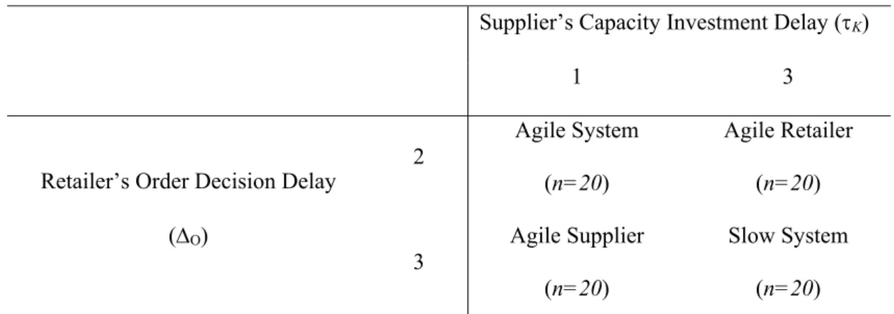
build capacity. We run a full experimental design, with four experimental treatments. The first treatment (T1) presents an agile system. This is the system with less dynamics in our experiments, where we account for the lowest value in our experimental variables. The forth treatment (T4) is the most dynamically complex system (slow system), where our experimental variables take the highest possible value. Treatment 2 (T2) presents an agile retailer with a slow supplier, where we combine short retailer ordering delay and a long supplier capacity acquisition delay. Finally, Treatment 3 (T3) presents only an agile supplier with a slow retailer, where we combine short supplier capacity acquisition delay with a long retailer ordering delay. Table 2.1 characterizes each treatment conducted and the number of participants (n) in each treatment.
2.3.2. Experimental Protocol
We followed the standard experimental economics protocol (see Friedman & Sunder, 1994, 2004). Subjects were fourth and fifth year Industrial and Management Engineering students at the National University of Colombia, in the autumn of 2010. Subjects did not have previous experience in any related experiment.
Table 2.1. Experimental treatments
Supplier’s Capacity Investment Delay (K)
1 3
Retailer’s Order Decision Delay (O) 2 Agile System (n=20) Agile Retailer (n=20) 3 Agile Supplier (n=20) Slow System (n=20)
Participants were told they would earn a show-up fee of Col$10.000 (approximately US$5) and a variable amount contingent on their performance, between Col$0 and Col$30.000 (US$0 - US$15) for an overall average payoff of Col$24.000 (US$12). The experiment ran for around one hour and students were informed about the duration of the experiment beforehand. The payoff was more than two times larger than the opportunity cost for an undergraduate student in a public university in Colombia. The students were also given a set of instructions describing the production system, the decisions and the goals of the game (shown in detail in Appendix 2.2).
We ran the experiment with 20 subjects per treatment. Upon arrival, subjects were seated behind computers and one of the four treatments was assigned randomly (see Appendix 2.3). Participants were allowed to ask questions and test out the computer interface (see Appendix 2.4). All the experiment parameters were common knowledge to all participants. We ran the experiment using the computer simulation software Powersim-Constructor-2.51®. The software ran automatically and kept record of all variables, including subjects’ decisions. Subjects wrote their decisions on a sheet of paper, which served as a physical backup of the data.
2.3.3. Optimal Simulated Trajectory
To properly assess subjects’ performance, we compare their ordering behavior with the optimal simulated order trajectory in each treatment. These optimal order trajectories are estimated using the Solver in Powersim Studio 8 and minimizing the total cost over all periods. Powersim Studio 8 uses an optimization method called evolutionary search. Inspired by Darwin's evolutionary theory, the method is a goal-seeking process where successive runs take place and where the best inputs from a run are used in the next run to generate new inputs to a simulation and try to find the optimum.
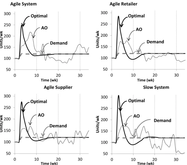
Figure 2.4
shows the behavior of these optimal trajectories (thick continuous line) in each treatment. The optimal ordering trajectories are characterized by a large initial order at the moment the demand surges. The magnitude of this optimal initial order increases with the complexity (longer delays) of the system. Then, orders exponentially decrease with a damped oscillation until settling into equilibrium. The magnitude of the damped oscillation increases with system complexity. Finally, optimal orders settle at 120 units per week for the rest of the trajectory.2.4. Results
In this section, we present the overall results of our experiments. Our experimental results are based on 61 subjects (15 in the agile-system treatment, 17 in agile-retailer treatment, 14 in the agile-supplier treatment and 15 in the slow-system treatment), chosen among all the subjects after excluding outliers. In order to identify outliers in our experiment, we use both qualitative and quantitative analyses. First, we identified the subjects that clearly did not understand the system; and then we conducted four different quantitative tests to remove the remaining extreme cases. In general, in our quantitative identification of outliers, we used different univariate methods as the ones presented by Ben-Gal (2005), Croson et. al. (2014) and Sterman and Dogan (2015).
2.4.1. Subjects’ Order Decisions Behavior
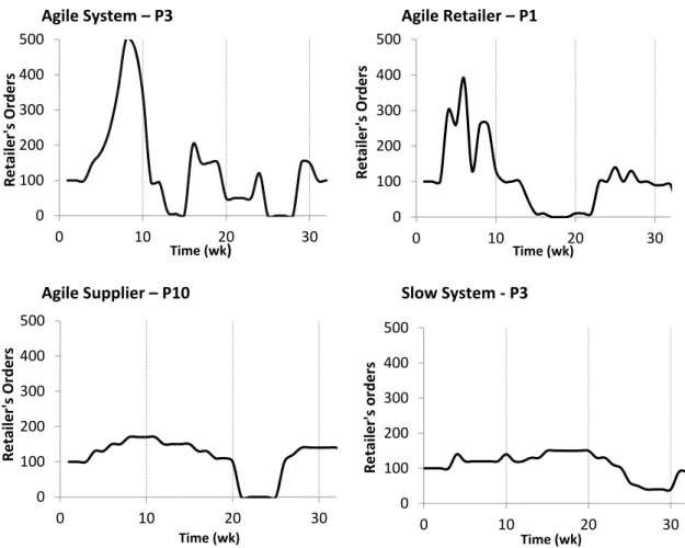
Subjects received information on the system structure, delays and costs (see Appendix 2.2 for the description of the instruction) and then were asked to place orders that would minimize total simulated long-run costs. Figure 2.3 shows ordering behavior for four selected subjects (one in each treatment) capturing typical behavior of subjects. The results suggest a common pattern: subjects’ orders initially
over-shoot, then under-shoot until settling around equilibrium close to 120 units (the final customer demand). Agile System – P3 Agile Retailer – P1 Agile Supplier – P10 Slow System ‐ P3
Figure 2.3. Typical experimental results (Pj indicates the subject ID with j=1, … 15).
Figure 2.3 also shows that subjects in the agile-system and agile-retailer treatments (with shorter ordering delays) over-order for shorter periods of time (around 10 weeks) compared with subjects in the agile-supplier and slow-system treatments who over-order for longer periods, but displays less variability. In the agile-system and agile-retailer treatments, the shorter ordering delays allowed subjects to more quickly adjust their orders. To compare overall subject behavior in each treatment with the optimal ordering decisions, we compute the average retailer´s orders (AO) for players in each treatment. Figure 2.4 suggests that subjects fail to place sufficiently large initial orders, and also fail to reduce them quickly toward the equilibrium value. Instead, subjects place orders with magnitudes averaging half of the desired initial value, but maintain high orders for a longer period than desired. When subjects finally reduce their orders, they do so more than the optimal values. As a result, subjects’ orders fluctuate around the optimal trajectory in all treatments. While the pattern presents similarities across treatments,
0 100 200 300 400 500 0 10 20 30 Retailer's Orders Time (wk) 0 100 200 300 400 500 0 10 20 30 Retailer's Orders Time (wk) 0 100 200 300 400 500 0 10 20 30 Retailer's Orders Time (wk) 0 100 200 300 400 500 0 10 20 30 Retailer's orders Time (wk)
it is also possible to identify differences. The high initial subjects’ orders tend to remain high for a longer period in treatments with longer retailer ordering delays (agile-supplier and slow-system treatments). Subjects’ decisions are less stable and take longer to settle in the treatment with higher delays (slow-system treatment).
Agile System Agile Retailer
Agile Supplier Slow System
Figure 2.4. Final customer demand, optimal and average subjects’ orders (AO) in each treatment.
2.4.2. Subjects’ Cost Performance
The subjects’ main objective in the experiment was to minimize cumulative costs. Table 2.2 presents total cumulative costs per subject and the average, the median, the minimum and the optimal for each treatment. A general observation is that most of the subjects perform far from optimal for all treatments. The lowest total cost achieved by a subject was 20% higher than the optimal of the treatment, which occurred for subject P12 in the agile-retailer treatment. The best performances observed in the other treatments were also above optimal costs: 32% above optimal in the agile-system treatment, 37% above optimal in the agile-supplier treatment and 95% above optimal in the slow-system treatment.
50 100 150 200 250 300 0 10 20 30 Units/wk Time (wk) AO Optimal Demand 50 100 150 200 250 300 0 10 20 30 Units/wk Time (wk) AO Optimal Demand 50 100 150 200 250 300 0 10 20 30 Units/wk Time (wk) AO Optimal Demand 50 100 150 200 250 300 0 10 20 30 Units/wk Time (wk) AO Optimal Demand
Table 2.2. Total cumulative, average, and optimal costs across treatment for the experiment Subject Agile System ($) Agile Retailer ($) Agile Supplier ($) Slow System ($) P1 2,331.95 3,243.45 1,285.69 1,576.23 P2 16,186.75 10,474.18 6,349.57 1,976.48 P3 17,921.82 1,313.24 1,439.31 19,297.83 P4 3,995.25 6,806.07 2,441.01 12,619.97 P5 845.60 3,017.32 1,407.55 30,220.81 P6 3,834.15 878.90 2,086.54 4,258.17 P7 6,805.24 899.15 3,946.30 2,214.28 P8 25,358.16 14,624.58 2,410.65 1,403.54 P9 4,056.73 2,712.87 2,958.85 2,294.44 P10 1,664.46 854.73 1,202.67 2,649.15 P11 1,511.78 10,944.48 1,106.48 13,445.40 P12 1,193.47 781.92 885.04 35,200.88 P13 4,790.34 2,438.42 961.68 1,388.21 P14 805.86 1,002.29 1,719.34 5,960.91 P15 27,068.96 2,792.65 16,640.05 P16 7,144.60 P17 5,362.77 Average (Standard Error) 7,891.37 (2344,72) 4,428.92 (1018,97) 2,157.19 (396,83) 10,076.42 (2845,09) Median 3,995.25 2,792.65 1,579.33 4,258.17 Min 805.86 781.92 885.04 1,388.21 Optimal 610.94 654.99 646.86 712.50 Min/Optimal 1.32 1.20 1.37 1.95
Subjects’ average performances vary from 333% to 1414% higher than the optimal. These results are conservative since we have excluded subjects with outlying ordering behavior, who present even higher costs (including outliers we get average values of $23,312.73; $6,792.49; $4,724.34 and $13,551.26 for treatments 1 to 4 respectively). The lowest optimal costs is observed in the agile-system treatment ($610.94) and highest is in the slow-system treatment ($712.50), these results highlight the increasing system difficulty when higher delays are introduced producing lower performances. In general, subjects’ decisions present higher total cumulative cost in the less agile system (slow-system treatment). In addition, results from the agile-retailer and agile-supplier treatmentspresent lower total cumulative costs than results from the slow-system, as expected. However, results in the agile system do not completely fit the pattern expected if we think shorter time delays will lead to lower total cumulative costs. In this case, both the average and median costs in the agile-system treatment are higher than the average and median cost of the agile-retailerand agile-supplier treatments. This could have a methodological explanation. For example, we could have improved the experimental design, emphasizing higher difference in delays among treatments. Probably, under the lack of large enough sample size, the current setup does not allow us to identify significant differences in costs among treatments and the potential unexpected results could be given just by a normal increase in the orders’ variability or a potential sampling selection problem in one of the treatments (in this case the agile-system treatment).
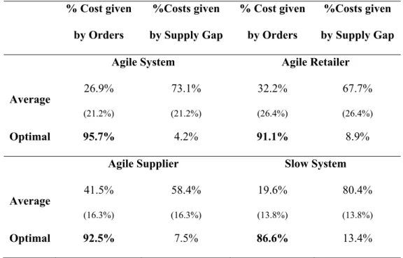
Table 2.3 shows how cost components contribute to optimal and average subjects’ total cost in each treatment. These results are robust to changes in cost parameters. The cost breakdown in the optimal trajectory suggests that most of the costs are given by the ordering component. Hence, the choice of parameters
and
induce optimal orders that minimize the Supply Gap and its associated cost. In contrast, the cost breakdown for the subjects’ decisions shows that subjects have difficulties balancing supply and demand, placing orders that fail to minimize the Supply Gap. Thus, a disproportionally high fraction of the subjects’ costs is due to the Supply Gap cost component. As expected, in the most dynamically complex treatment (slow-system treatment), subjects incur the highest proportion of costs due to the Supply Gap. These results are also conservative, because if we include outliers, the costpercentage given by the Supply Gap will be higher (76.04% for the agile system, 69.38% for the agile retailer, 65.12% for the agile supplier and 82.49% the slow system). This is because the level of underperformance was higher in those subjects excluded from the analysis meaning that, their capacity to minimize the Supply Gap was even lower.
Table 2.3. Costs distribution given by Orders and Supply gap
% Cost given by Orders %Costs given by Supply Gap % Cost given by Orders %Costs given by Supply Gap
Agile System Agile Retailer
Average 26.9% (21.2%) 73.1% (21.2%) 32.2% (26.4%) 67.7% (26.4%) Optimal 95.7% 4.2% 91.1% 8.9%
Agile Supplier Slow System
Average 41.5% (16.3%) 58.4% (16.3%) 19.6% (13.8%) 80.4% (13.8%) Optimal 92.5% 7.5% 86.6% 13.4%
Standard Deviation in parenthesis
Given the qualitative similarity of the decision patterns and the results shown in this section, one might argue that subjects use a heuristic with common features in order to make their orders (Sterman, 1989a). In the next section, we discuss a specific decision rule and test the accuracy of the rule using econometrical analyses.
2.5. Modeling Decision Rules
For modeling the subjects’ decision rules, we test the heuristic (equation (2.9)) proposed by Gonçalves (2003). Gonçalves modeled retailer’s orders, RD, using an anchor and adjustment heuristic, where the retailer anchors its orders on a demand forecast, and then adjust it up or down to maintain orders at a desired level. The anchor term captures retailer’s intention to place sufficient orders to meet their customers’ orders. The adjustment term closes the gap between retailer’s desired and actual backlog of orders within a specific adjustment time. Gonçalves (2003) also assumes that each retailer adopts the same heuristic with the model capturing total values for customer demand forecast (d), actual backlog
of orders (B), desired backlog of orders (B*), and adjustment time
B). Finally, total retailer’s orders are non-negative (no cancellations).
B DB
B
d
Max
R
*,
0
(2.9)Where, retailer’s desired backlog of orders (B*) is given by the product of the demand forecast (d) and the expected delivery delay to receive orders from the supplier (ED).
ED d
B* (2.10)
Now, let’s assume that the expected delivery delay is given by a linear function of the actual delivery delay (AD) with slope .This function captures retailer’s delivery delay adjustment, that is, when faced with long delivery delays, a retailer sets its expected delivery delay (ED) above the actual delivery delay (AD) quoted by the supplier. Longer expected delivery delays (ED) rather than actual (AD) leads to higher desired backlog of orders (B*) and higher retailer’s orders.
ED = α AD, where α≥1 (2.11)
Where, actual delivery delay (AD) is given by the ratio of the order backlog (B) to shipments (S). Substituting equations (2.10) and (2.11) into (2.9), we obtain equation (2.12), which can be used as a heuristic to test if retailers’ orders are well represented by an anchoring and adjustment heuristic.
B DB
K
B
d
d
Max
R
,
0
(2.12)The system determined by equation (2.12) involves a nonlinearity associated with the ratio of the two states: order backlog (B) and capacity (K). As proposed in Gonçalves and Arango (2010), we linearize the system using a Taylor series approximation of the ratio of the two states (B/K) around the initial backlog (B0) and capacity (K0) and neglect higher order terms (details of the linearization process can be found in Appendix 2.5). We get a linear approximation of the anchor and adjustment heuristic, which can be tested econometrically:
B
K
K
d
K
K
d
d
d
Max
R
B B D B D D 0 0 0,
0
(2.13)Below, we analyze this linearized heuristic using two different methods. First, in order to test if this linearized heuristic represents each subject behavior, we estimate the model coefficients for each subject in each treatment using least squares. Second, to test if the linearized heuristic is able to explain the general behavior, we structure the data as a panel estimating a single model for all subjects and treatments. The panel data estimation increases the efficiency of our estimate and its representativeness.
2.5.1. Least Squares Analysis
To econometrically analyze the model stated in equation (2.13), we first omit the maximum operator due to the low incidence of zero decision occurrences (~10%) within each subject’s decisions and then we make the following parameter substitutions:
B D
d
d
0
; 0 1K
d
B D
and 0 0 2K
K
d
B
(2.14)Then equation (2.13) can be re-written as:
tij t ij t ij ij Dtij
K
B
R
0
1
2
(2.15)Where
kij represents coefficient k, for subject i and treatment j, where k=0,1,2, i=0,1,…,15 and j=1,..., 4, and tijis the error term. The parameter values in equation (2.15) suggest that we should expect coefficient 0 to be positive
00
, 1 to be negative
10
, and 2 to be positive
20
. A positive coefficient for 0 is reasonable since this anchor is the sum of two positive terms. A negative coefficient for 1 is also intuitive since a higher value of supplier capacity (K) induces lower orders by the retailer. Finally, a positive coefficient for 2 suggests that faced with a large backlog (B) a retailer will order more in an attempt to receive what she needs. Substituting the parameter values used in the simulation model (D =10,B =4, K0=100, = 1.1 and d =120), we can obtain estimates for the:Table 2.4. Coefficient estimates
0 1 2
450 -3.3 0.08
We used the R software to obtain the estimates for the model in equation (2.15). Table 2.5 provides the results.
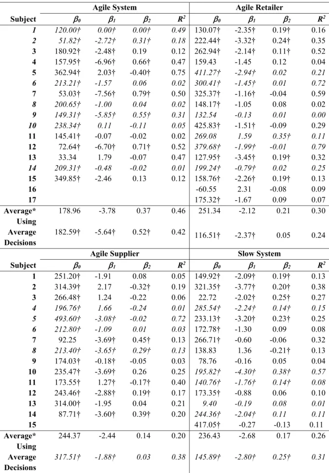
Table 2.5. Coefficient estimates of decision rule for each individual for all treatment
Agile System Agile Retailer
Subject 0 1 2 R2 0 1 2 R2 1 120.00† 0.00† 0.00† 0.49 130.07† -2.35† 0.19† 0.16 2 51.82† -2.72† 0.31† 0.18 222.44† -3.32† 0.24† 0.35 3 180.92† -2.48† 0.190 0.12 262.94† -2.14† 0.11† 0.52 4 157.95† -6.96† 0.66† 0.47 159.430 -1.450 0.120 0.04 5 362.94† 2.03† -0.40† 0.75 411.27† -2.94† 0.020 0.21 6 213.21† -1.570 0.060 0.02 300.41† -1.45† 0.010 0.72 7 53.03† -7.56† 0.79† 0.50 325.37† -1.16† -0.040 0.59 8 200.65† -1.000 0.040 0.02 148.17† -1.050 0.080 0.02 9 149.31† -5.85† 0.55† 0.31 132.540 -0.130 0.010 0.00 10 238.34† 0.110 -0.110 0.05 425.83† -1.51† -0.090 0.29 11 145.41† -0.070 -0.020 0.02 269.080 1.590 0.35† 0.11 12 72.64† -6.70† 0.71† 0.52 379.68† -1.99† -0.010 0.79 13 33.340 1.790 -0.070 0.47 127.95† -3.45† 0.19† 0.32 14 209.31† -0.480 -0.020 0.01 199.24† -0.79† 0.020 0.25 15 349.85† -2.460 0.130 0.12 158.76† -2.26† 0.19† 0.13 16 -60.550 2.310 -0.080 0.09 17 175.32† -1.670 0.090 0.07 Average* 178.96 -3.78 0.37 0.46 251.34 -2.12 0.21 0.30 Using Average Decisions 182.59† -5.64† 0.52† 0.42 116.51† -2.37† 0.05 0.24
Agile Supplier Slow System
Subject 0 1 2 R2 0 1 2 R2 1 251.20† -1.910 0.080 0.05 149.92† -2.09† 0.19† 0.13 2 314.39† 2.170 -0.32† 0.19 321.35† -3.77† 0.20† 0.38 3 266.48† 1.240 -0.220 0.06 22.720 -2.02† 0.25† 0.27 4 196.76† 1.660 -0.240 0.01 285.54† -2.24† 0.14† 0.15 5 493.60† -3.08† -0.020 0.72 233.13† -3.20† 0.23† 0.25 6 212.80† -1.090 0.010 0.03 172.78† -1.300 0.090 0.08 7 92.250 -3.69† 0.45† 0.13 266.71† -0.600 -0.060 0.32 8 213.40† -3.65† 0.29† 0.13 138.830 1.360 -0.21† 0.13 9 174.03† -0.18† -0.050 0.03 78.760 -0.160 0.050 0.04 10 235.47† -3.69† 0.260 0.25 195.82† -4.30† 0.38† 0.57 11 173.55† 1.27† -0.17† 0.40 140.76† -1.76† 0.14† 0.08 12 243.46† -2.88† 0.19† 0.17 173.35† -0.880 0.060 0.10 13 314.00† -1.950 0.040 0.21 9.400 -0.190 0.080 0.01 14 87.71† -3.60† 0.39† 0.20 244.36† -2.04† 0.110 0.11 15 417.05† -0.27 -0.13 0.11 Average* 244.37 -2.44 0.14 0.20 236.43 -2.68 0.17 0.26 Using Average Decisions 317.51† -1.88† 0.03 0.38 145.89† -2.80† 0.25† 0.31
Initially, we estimated the parameters for each subject using Ordinary Least Squares (OLS) and then, checked if the OLS assumptions were satisfied. In the cases where all the OLS assumptions were satisfied, those parameter estimations were kept. However, in some cases we found significant autocorrelation of the error term, which makes the OLS estimator inefficient. In the cases with significant autocorrelation of errors, the parameters were re-estimated using Generalized Least Squares with an Auto-Regressive model of order 1 (AR(1)) as model for the residuals. Table 2.5 also shows the method used in each regression. In addition, residual analyses do not show heteroskedasticity, so it is unlikely to bias estimation significantly.
In general, the estimations satisfied the OLS assumptions in 36% of the cases; in the remaining 64% of the cases, we had to use GLS. Results show that a high fraction of the estimated models is significant. For instance, we found significant values for all three parameters in 38% of all subjects and that more than 30% of R2 values are larger than 0.30. Table 2.5 also computes the R2 of the “average decision rule” obtained running the model using the average decisions for each treatment (ranging between 0.24 and 0.47), which in social sciences are considered as a moderate explanation. However, these results are not completely conclusive. While the proposed decision rule is consistent for some of our subjects, it is not able to explain subjects’ behavior in other cases. For instance, we have a R2 lower than 0.2 in 60% of the cases. This suggests that individuals could be using different strategies to make their ordering decisions. Some subjects could be using a rule that combines forecasting and feedback structures as proposed by Paich and Sterman (1993) or they could also be following a non-linear expectation rule or any classical discrete inventory control rule as presented by Barlas and Özevin (2004). However, analyzing the accuracy of these alternative heuristics goes beyond the scope of this study.
In addition, considering the specific results for each coefficient, we observe that the constant β0 is positive and significant for 83% of all subjects. Coefficient β1 is also consistent with our expectations, with negative and significant values for most subjects. More specifically, we find significant values for β1 in 53%, 65%, 57%, and 53% of subjects in the agile-system, agile-retailer, agile-supplier and slow-system treatments, respectively. In addition, most of the signs (83%) of β1 are negative and 62% of them are significant. The estimates obtained for coefficient β2 are also as expected with positive values for
most subjects (70%), and β2 has significant values for 47%, 35%, 42%, and 53% of subjects in the agile-system, agile-retailer, agile-supplier and slow-system treatments, respectively. Most of the signs (70%) of β2 are positive and 53% of them are significant. Table 2.5 also shows that, after using the least squares estimation with the average decisions, most of the parameters are significant (83%) and all of them have the right signs. (Our qualitative and quantitative analyses do not change significantly if we include outliers.) In addition, the average parameter estimation for each treatment also has the correct signs. Finally, running the model used in the experiment with the estimators obtained with each subject, does not return a single order for zero units. This result suggests that there is no violation of the non-negativity constraint (cancellations were not allowed during the experiment), which supports our estimation omitting the maximum operator in equation (2.13).
Comparing the parameter values for β1 and β2 (Table 2.5) with the expected values obtained using the linearized heuristic (Table 2.4), we see that the econometric estimations for β1 and β2 have the proper signs. In addition, the estimated value for β1 is fairly close to the value derived by the linearized heuristic (-3.3); however, the estimated value found for β2 is farther from the expected one. This result could be given by non-significant estimations, due to an expected β2 value that is close to zero (0.08) and a limited time series (35 periods). However, if we consider the average of all β2 coefficients (both significant and insignificant), we obtain a value of 0.11, which is close to the expected value of β2 (0.08).
Finally, for a few subjects we find statistically significant estimates for parameters β1 and β2 with unexpected signs. This is the case for four players: P5 in the system treatment, P2 and P11 in agile-supplier treatment, and P8 in the slow-system treatment. These switches in parameter signs could have occurred because those subjects were able to place high orders at the very beginning of the experiment, when the backlog was relatively low (changing the sign of β2). Then, β1 had to control (at least weakly) for the subjects’ order increments presented in the remainder of the experiment. These results could also mean that subjects may be using a different decision rule or that they change their decision rule over time. Alternatively, subjects could be using a dynamic decision rule as the one presented by Sterman and Dogan (2015).
To more deeply investigate our understanding of human behavior and the effectiveness of our heuristic, we analyze the data using a panel data analysis. This allows us to get information about the collective subject behavior, controlling for subjects’ individual effects.
2.5.2. Panel Data Analysis
We structure the data from the experiments as a panel to control for omitted variables that vary over time but are constant between subjects in each treatment (e.g., temperature, time of the day, day of the week, etc.) and to account for individual heterogeneity, controlling for variables that cannot be observed or measured (e.g., cultural factors). The panel increases the efficiency of the estimations of the linearized model and improves the potential representativeness of the decision rule.
Before making the panel data analysis, we had to decide whether to use random effects, fixed effects, or simple (pooling) least squares. The Breusch Pagan Lagrange multiplier (BP-LM) test helps us decide between random effects and a simple regression. After running this test for each treatment, we found significant difference across subjects (i.e. panel effect): Prob > Chi2 is 0.00 all for treatments,
which allows us to conclude that random effects are more appropriate.
Next, we run a Hausman test to decide between random or fixed effects. This test checks whether the unique errors are correlated with the regressors. If the effects are exogenous, random effect is efficient, and the fixed effect is just consistent; therefore, we should use random effects. However, if the effects are not exogenous, the fixed effect is efficient, and the random effect is biased, we should use fixed effects. After running the Hausman test for each treatment as a null hypothesis with the preferred model as random effects (and as an alternative to the fixed effects), we found significant differences in all treatments: Prob > Chi2 is less than 0.1 (0.00 for the agile-system, agile-supplier and slow-system
treatments, and 0.095 for the agile-retailer treatment). Hence, we can reject the null hypothesis and adopt fixed effects as the appropriate approach. To explain overall subjects’ behavior, we also control for time-fixed effects. Table 2.6 provides the results of the panel data analysis using Stata.
The significance test of the model using the statistic F shows that all the p -values are small (p-values ~0.00) suggesting that the proposed model (of the linearized heuristic) is an acceptable way for explaining subjects’ ordering decisions. Table 2.6 also shows the R2 for each treatment. The proposed
on average the 25% of the variability in subjects’ behavior. In addition, the heuristic performs better explaining subjects’ decision when the retailer’s order decision delay is low (system and agile-retailer treatments).
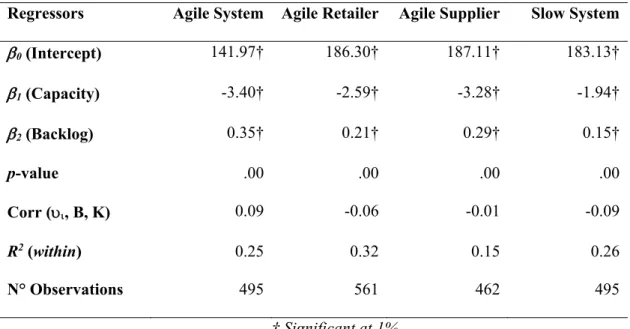
Table 2.6. Coefficient estimates of decision rule for treatment as panel data
Regressors Agile System Agile Retailer Agile Supplier Slow System
0 (Intercept) 141.97† 186.30† 187.11† 183.13† 1 (Capacity) -3.40† -2.59† -3.28† -1.94† 2 (Backlog) 0.35† 0.21† 0.29† 0.15† p-value .00 .00 .00 .00 Corr (, B, K) 0.09 -0.06 -0.01 -0.09 R2 (within) 0.25 0.32 0.15 0.26 N° Observations 495 561 462 495 † Significant at 1%
Furthermore, the three coefficients in all treatments are all highly significant and have the expected signs. The 1 coefficients are negative and with the expected value (Table 2.4 & Table 2.6). The 2 coefficients are positive for all treatments as expected, however, the estimated values overestimate the expected magnitude 2 to 4 times (Table 2.4 & Table 2.6). A possible explanation for the overestimation of 2 may be due to the complexity of the task. In particular, subjects overestimate
2 to compensate for the underestimation they make for 0 (the anchor in the linearized heuristic). Additional insight (that we could not do with the cost analyses - see Table 2.2) could be obtained now from the parameter estimates. Initially, the 1 estimation in the agile-system treatment (-3.40) and
the agile-retailer treatment (-2.59) are lower than the estimations in the agile-supplier treatment (-3.28) and the slow-system treatment (-1.94), respectively. This could mean that subjects take into account the supplier’s capacity investment delay and do not need to inflate their orders when the supplier is able to quickly satisfy their orders (K = 1). Similarly, the 1 estimation in the agile-system treatment (-3.40)
and the agile-supplier treatment 3.28) are lower than the estimations in the agile-retailer treatment (-2.59) and the slow-system treatment (-1.94), respectively. This means that subjects are accounting for
the effect of their ordering decision delay and they increase their orders when their orders take longer to be perceived by the supplier (O = 3). A similar analysis can be done for the effect of 2 and the
experimental variables in subjects’ ordering decisions. Hence, despite the cost analyses do not show a clear consistency on some results (especially for the agile system), the panel estimation allows us to see some consistency about how accurately subjects could be making their decisions, taking into account the effect of our experimental variables.
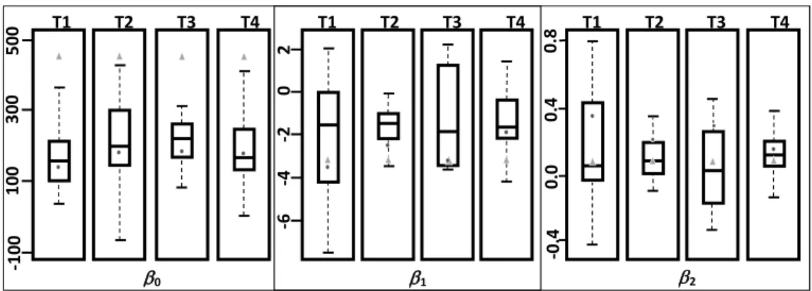
Figure 2.5 summarizes the results obtained in the previous sections. First, we build box-plots using the estimated parameters, obtained by least squares, for all subjects in each treatment (Table 2.5). Second, we let triangles represent the expected values of the linearized heuristic (Table 2.4). Finally, we capture the panel data estimations with circles (Table 2.6). The box-plots show the general ranges and distribution for each parameter, indicating whether (or not) they are skewed. In comparing the results, it is important to note the different scales for parameters 0, 1 and 2. Overall we note that estimates obtained by OLS or GLS, and those obtained by the panel data are similar for all coefficients. However, the panel data estimates for 1 are closer to the expected values, and the OLS & GLS estimates for 2 are closer to the expected values. We also note that subjects underestimate 0 in all treatments, that is, econometrically estimated 0 coefficients are lower than the expected values of the linearized heuristic. Subjects tend to underestimate 1 (values closer to 0) in all treatments.
Figure 2.5. Box plots with the coefficient estimations using least squares, expected values (triangle), and panel data estimations (circle).
Figure 2.5 also shows that 63% of the expected values and panel data estimations are between the first and third quartile of the individual least square estimations (represented with the boxplots) in all treatments (T1: agile system, T2: agile retailer, T3: agile supplier and T4: slow system). This percentage
‐0.4 0.0 0.4 0.8 ‐4 ‐2 0 2 ‐100 100 300 500 T1 T2 T3 T4 T1 T2 T3 T4 T1 T2 T3 T4 ‐6 0 1 2
is not higher because the expected values of are higher than the experimental results, meaning that the heuristic is creating an overestimation of the independent parameter. However, the results for 1 (Capacity coefficient) and 2 (Backlog coefficient) show that the estimated values using the heuristic and the panel data analysis are generally with the right sign and also within the expected range.
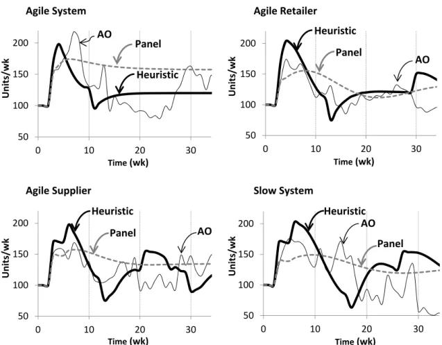
Figure 2.6 shows that the AO estimations in the agile-system and agile-supplier treatments (those with lower supplier capacity investment delay) present higher variability, increasing the uncertainty in parameter estimation. This increase in variability means that when subjects (as retailers) are able to get a faster response from their supplier, they present more unpredictable behavior, which affects the supplier’s planning. Estimations in the agile-retailer and the slow-system treatments show that subjects are more consistent in their decisions, increasing predictability in their behavior.
Agile System Agile Retailer
Agile Supplier Slow System
Figure 2.6. Average subjects’ orders (AO), simulation of the proposed heuristic (Heuristic), adjusted model with panel parameters (Panel).
Using the estimators obtained with the panel data analysis (Panel), we inserted and ran them into the same model of the experiment. Figure 2.6 shows the behavior of these runs over time. As it was
50 100 150 200 0 10 20 30 Units/wk Time(wk) AO Panel Heuristic 50 100 150 200 0 10 20 30 Units/wk Time(wk) AO Panel Heuristic 50 100 150 200 0 10 20 30 Units/wk Time(wk) AO Panel Heuristic 50 100 150 200 0 10 20 30 Units/wk Time(wk) AO Panel Heuristic