A cautionary tale about control variables in IV estimation

W

ORKING

P

APERS

SES

F

S

E

S

W

-

S

F

U

F

| U

F

12.2014

N° 453

A cautionary tale about control

variables in IV estimation

A cautionary tale about control variables in IV estimation

Eva Deuchert* and Martin Huber+

* University of St. Gallen, School of Economics and Political Sciences + University of Fribourg, Department of Economics

Abstract: Many instrumental variable (IV) regressions include control variables to justify (conditional) independence of the instrument and the potential outcomes. The plausibility of conditional IV independence crucially depends on the timing when the control variables are determined. This paper systemically works through different IV models and discusses the (conditions for the) satisfaction of conditional IV independence when controlling for covariates measured (a) prior to the instrument, (b) after the treatment, or (c) both. To illustrate these identification issues, we consider an empirical application using the Vietnam War draft risk as instrument either for veteran status or education to estimate the effects of these variables on labor market and health outcomes.

Keywords: instrument, control variables, conditional independence, covariates JEL classification: C26, J24

We have benefitted from comments by Dionissi Aliprantis, Per Johansson, and seminar participants in

Aarhus, Linz, and Bludenz. Corresponding author: Martin Huber ([email protected]), University of

Fribourg, Department of Economics, Bd. de Pérolles 90, 1700 Fribourg, Switzerland.

1 Introduction

The evaluation of causal effects in empirical economics frequently relies on instrumental variable (IV) methods. Identification requires that the instrument is associated with the (supposedly) endogenous treatment variable (IV relevance), but is not directly related with the outcome or unobservables affecting the outcome (IV validity). In many empirical applications, the latter assumption occurs only reasonable when controlling for further covariates, often referred to as conditional IV independence.

It is remarkable that in many IV studies, the discussion and justification of conditional IV independence does not pay much attention to the time period in which the control variables are measured, i.e. whether this happens prior to instrument assignment or at a later point. In particular, there seems to exist a wide spread (tacit) consensus that it is reasonable to use IV methods in cross sectional data, where outcomes and controls are measured in the same period. This stands in stark contrast with the program evaluation literature relying on conditional independence of the treatment (rather than the instrument) given observed controls, where it is well acknowledged that credible controls need to be measured prior to treatment assignment. Otherwise, they might be affected by (i.e. be an outcome of) the treatment so that conditioning on them likely introduces selection bias (e.g., Rosenbaum, 1984; Lechner, 2008).

In this paper we use graphical tools (so-called causal diagrams, see Pearl, 1995) to discuss various IV models that postulate different causal relations between pre-instrument covariates, the instrument, the treatment, post-treatment covariates, and the outcome. For each scenario, we demonstrate whether treatment effects may be identified by IV methods when conditioning on pre-instrument covariates, post-treatment covariates, or both. This framework allows us to show that the timing of the measurement of controls – albeit often ignored in the literature –

crucially affects the plausibility of conditional IV independence and provides a simple guideline for selecting control variables in conditional IV frameworks.

We identify three crucial conditions for the validity of conditional IV strategies: (i) Pre-instrument covariates have no direct effect on outcomes (other than through observed post-treatment covariates) and are not associated with unobservables affecting the outcome, (ii) post-treatment covariates are not confounded by unobservables, and (iii) the instrument does not directly affect any post-treatment variables (other than through the treatment of interest). Only if all three conditions jointly hold, controlling for either pre-instrument or post-treatment covariates (which may more easily observed in practice) both yield causal effects. If any of assumptions (i) to (iii) is violated, the point in time in which the covariates are determined is crucial. In some cases, it is necessary to control for pre-treatment covariates, post-treatment covariates, or even both. Moreover, identification is lost irrespective of the chosen controls, namely if the instrument affects post-treatment covariates and the latter are confounded by unobservables so that assumptions (ii) and (iii) are jointly violated.

We use the well-known Vietnam War draft risk as an illustrative example for different conditional instrumental variable strategies. During the Vietnam War, the majority of American troops consisted of volunteers, the rest were selected for military service through a draft (Gimbel & Booth, 1996). The draft had two important consequences for young men: On the one hand it increased the probability of joining the army, either through induction or volunteering due to expectedly better terms of service (Angrist J. D., 1991). On the other hand, education deferment induced higher college enrollment among the civilian population (Card & Lemieux, 2001). Several authors use the draft risk as an instrument either for military status or for college education, to estimate the effect of these variables on various outcomes (for example Angrist J. D., 1990; Conley & Heerwig, 2012; Dobkin & Shabani, 2009; Grimard & Parent, 2007; Lindo & Stoecker, 2014; Malamud & Wozniak, 2010; de Walque,

2007). We reconsider this instrument to discuss under which conditions causal effects can be estimated using conditional IV strategies and use survey data collected shortly before and after individuals were at risk to be drafted to demonstrate that these conditions are unlikely to hold in reality.

The remainder of this paper is organized as follows. Section 2 introduces a general IV model along with the conditional IV independence assumption as a precondition for identification. Section 3 describes the Vietnam draft and outlines how previous research used the Vietnam draft risk in conditional IV settings. Section 4 uses causal diagrams to define various IV models that differ in terms of causal relations between observed and unobserved variables. For each case, it discusses whether conditional IV independence holds and treatment effects can be identified when controlling for pre-instrument covariates, post-treatment covariates, or both. Section 5 provides an empirical illustration where different conditional IV strategies are employed to estimate the effect of veteran status or education on labor market and health outcomes. The final section concludes.

2 A general IV model

Assume we are interested in the effect of a scalar endogenous treatment (denoted by 𝐷𝐷) on an outcome (𝑌𝑌) and have available a scalar instrument (𝑍𝑍). We consider the following IV model which is quite general in terms of functional forms of the outcome and treatment equations and therefore naturally allows for heterogeneous treatment effects w.r.t. observed and unobserved characteristics:

𝑌𝑌 = 𝜙𝜙(𝐷𝐷, 𝑋𝑋, 𝑈𝑈),

𝐷𝐷 = 𝜂𝜂(𝑍𝑍, 𝑋𝑋, 𝑉𝑉), (1) where 𝜙𝜙 and 𝜂𝜂 are unknown functions. 𝑋𝑋 denotes a vector pre-instrument covariates while 𝑈𝑈 and 𝑉𝑉 are the unobserved terms which may be arbitrarily associated with each other, thus

causing the treatment to be endogenous. Potential outcomes as a function of the treatment, 𝑌𝑌(𝑑𝑑), and potential treatment states as a function of the instrument, 𝐷𝐷(𝑧𝑧), see for instance the notation in Angrist, Imbens and Rubin (1996), are obtained by fixing the treatment and the instrument to particular values 𝐷𝐷 = 𝑑𝑑 and 𝑍𝑍 = 𝑧𝑧:

𝑌𝑌(𝑑𝑑) = 𝜙𝜙(𝑑𝑑, 𝑋𝑋, 𝑈𝑈), 𝐷𝐷(𝑧𝑧) = 𝜂𝜂(𝑧𝑧, 𝑋𝑋, 𝑉𝑉).

This is convenient for defining causal effects, as for instance the average treatment effects in the entire population, 𝐸𝐸[𝑌𝑌(1) − 𝑌𝑌(0)], or in a particular subpopulation (denoted by 𝑆𝑆), 𝐸𝐸[𝑌𝑌(1) − 𝑌𝑌(0)|𝑆𝑆].

Identification of potential outcomes and causal effects generally requires some conditional independence assumption between 𝑍𝑍 and the unobserved terms, often referred to as IV validity. Heckman and Vytlacil (2005), among many others, assume for instance that the instrument is conditionally independent of the unobserved terms given 𝑋𝑋:

𝑍𝑍 ⊥ { 𝑈𝑈, 𝑉𝑉 }|𝑋𝑋, (2)

where `⊥' denotes statistical independence. An implication of this assumption is 𝐶𝐶𝐶𝐶𝐶𝐶(𝑍𝑍, 𝑈𝑈|𝑋𝑋) = 0, which is sufficient for IV validity in the linear homogenous treatment effect model with 𝑌𝑌 = 𝐷𝐷𝛽𝛽_𝐷𝐷+ 𝑋𝑋′𝛽𝛽_𝑋𝑋+ 𝑈𝑈 and 𝐷𝐷 = 𝑍𝑍𝛼𝛼_𝑍𝑍+ 𝑋𝑋′𝛼𝛼_𝑋𝑋+ 𝑉𝑉 (in this case 𝑋𝑋 includes a constant and 𝛽𝛽_𝑋𝑋, 𝛽𝛽_𝐷𝐷, 𝛼𝛼_𝑍𝑍, and 𝛼𝛼_𝑋𝑋 denote the various coefficients). In terms of potential outcome notation, equation (2) implies that the instrument is conditionally independent of the potential treatment states and outcomes:

𝑍𝑍 ⊥ {𝑌𝑌(𝑑𝑑), 𝐷𝐷(𝑧𝑧)}|𝑋𝑋 for all d, z in the support of 𝐷𝐷, 𝑍𝑍, (3) see for instance Abadie (2003).

Identification is only obtained if equation (3) is supplemented by further restrictions, e.g. on either the relation of 𝐷𝐷 and 𝑍𝑍, 𝐷𝐷 and V, or 𝑈𝑈 (or a combination thereof). For instance, considering the case of a binary treatment, Abadie (2003) assumes that 𝐷𝐷 is weakly monotonic in 𝑍𝑍 given 𝑋𝑋 for all individuals and strictly monotonic given 𝑋𝑋 for some.1 This allows identifying (local) average or quantile treatment effects (LATE, LQTE) among compliers, the subpopulation whose treatment reacts on the instrument.2,3 In linear models, monotonicity is trivially satisfied if the first stage coefficient 𝛼𝛼_𝑍𝑍 in the regression of 𝐷𝐷 on 𝑍𝑍 is homogeneous. If homogeneity also holds w.r.t. the treatment coefficient 𝛽𝛽_𝐷𝐷, then even the average treatment effect in the population (ATE) is identified.

In this paper, we are agnostic about any of these further assumptions and exclusively focus on the implications and plausibility of conditional IV independence in various casual models. In this context, it is important to note that in many data sets where IV methods are used, observed variables (outcome, treatment, instrument, and covariates) are measured at the same point in time, as in cross sections. Therefore, rather than observing the covariates 𝑋𝑋 prior to instrument assignment, the covariates actually available in the data, which we denote by 𝐶𝐶, may or may not correspond to the pre-instrument values, depending on whether they are time-varying or not. It follows that studies invoking conditional IV independence in cross sectional data effectively rely on the following assumption:

𝑍𝑍 ⊥ {𝑌𝑌(𝑑𝑑), 𝐷𝐷(𝑧𝑧)}|𝐶𝐶 for all d, z in the support of 𝐷𝐷, 𝑍𝑍. (4)

1 _{An unconditional form of the monotonicity assumption was first postulated by Imbens and Angrist (1994) and}

Angrist, Imbens and Rubin (1996).

2 _{Vytlacil (2002) has shown that monotonicity is equivalent to the existence of a latent index representation for}

the treatment equation (see for instance Heckman and Vytlacil 2005): 𝜂𝜂(𝑍𝑍, 𝑋𝑋, 𝑉𝑉) = 𝐼𝐼{𝑚𝑚(𝑍𝑍, 𝑋𝑋) > 𝑞𝑞(𝑉𝑉)}, where 𝑚𝑚, 𝑞𝑞 are unknown functions and 𝐼𝐼{𝐴𝐴} denotes the indicator function (which is equal to one if 𝐴𝐴 is satisfied and zero otherwise). In contrast, Chernozhukov and Hansen (2005) do not assume monotonicity and relax (3) to 𝑍𝑍 ⊥ 𝑈𝑈|𝑋𝑋, but require instead that 𝑈𝑈 is identically distributed across 𝐷𝐷 given 𝑍𝑍, 𝑋𝑋, 𝑉𝑉 for the identification of quantile treatment effects.

3 _{Kasy (2013) shows (however, for the unconditional case without covariates 𝑋𝑋) that for a continuous 𝐷𝐷, strict}

monotonicity of the treatment in a (continuous) instrument along with the independence of the latter and the unobserved terms allows identifying causal effects, given that particular support conditions are met. As an alternative set of assumptions, Imbens and Newey (2009) assume strict monotonicity of 𝐷𝐷 in 𝑉𝑉 (rather than 𝑍𝑍), which is restricted to be a continuously distributed scalar with a strictly increasing distribution function.

6

Only if all covariates are time-constant (i.e. 𝑋𝑋 = 𝐶𝐶) is equation (4) equivalent to (3), a case unlikely to hold in many applications. For this reason, we clarify in a first step which causal effects may be identified in various models that all are consistent with (4). Depending on the timing of covariate measurement, (4) does not necessarily imply that the full or total causal effect of interest – which might (depending on other assumptions imposed) for instance be the LATE or (under stronger homogeneity restrictions) the ATE – is recovered. That is, the assumption may be satisfied even if only a partial causal effect is identified. Secondly, we critically assess the plausibility of (4) when partially or fully conditioning on post-treatment covariates, as it is often the case in IV estimation using cross sectional data. In particular, we discuss a range of causal models that generally violate IV independence in a cross section due to the absence of information about the chronological order of the variables involved. Thirdly, we also discuss models in which conditioning on post-treatment covariates is required to control for direct effects of instrument on outcomes (which would otherwise violate the IV exclusion restriction).

3 The Vietnam War draft

During the Vietnam War, the majority of American troops consisted of volunteers, while the rest were selected through a draft (Gimbel & Booth, 1996). Young men at age 18 had to register at local draft boards for classification. These boards determined medical fitness and decided on the order in which registrants would be called. Men who had physical problems, were attending college, or were needed to support their families were granted deferments. Many men receiving deferments were from wealthy and educated families. As a consequence, most soldiers drafted were men from poor and working-class families.

In an attempt to make the draft more equal, a draft lottery was conducted in the years 1969 to 1972 to determine the order of call to military service in for men born between 1944 and

1952. The lottery assigned a draft number to each birth date for men in certain age cohorts, where low draft numbers were called first. At the time of the lottery, the total manpower needs were not known. As a consequence, during most of the year the ultimate ceiling below which people were drafted was unclear. Ex-ante, lottery numbers can thus be seen as an important component of the draft risk.

This uncertainty in the ultimate ceiling may have caused important behavioral responses: On the one hand, education deferments were continued to be issued until 1971, which means that men could avoid being drafted by going to or staying in college (Card & Lemieux, 2001). On the other hand, low draft numbers may have not only increased the risk to be drafted but also increased the likelihood to voluntarily join the army. Previous research shows that low draft numbers are strongly associated with enlistment (Angrist J. D., 1991). Joining the army voluntarily came with better terms, for example through the possibility to choose the military branch and the timing of entry into service, as well as to accomplish special training or officer candidate programs. However, this came at the cost of longer duty (three to four years under voluntary enlistment vs. two years under the draft).

The Vietnam War draft risk has been used for IV-based estimation in many empirical applications. Several studies constructed instruments as functions of draft lottery numbers, such as the lottery-determined draft-eligibility status, that is an indicator for the lottery number being below the draft ceiling in a given year (e.g., Angrist J. D., 1990; Conley & Heerwig, 2011; Dobkin & Shabani, 2009; Lindo & Stoecker, 2014), or by grouping lottery numbers into several categories (Angrist & Krueger, 1992; Angrist & Chen, 2011; Angrist, Chen, & Frandsen, 2010). Note that making use of the draft lottery number requires information on the exact birth date of each respondent, which is often not provided in publicly available data sources for data protection reasons. A related instrument that does not rely on

the exact birth date is the draft risk faced by each birth cohort (e.g., de Walque, 2007; Grimard & Parent, 2007), or by cohort and state (e.g., Malamud & Wozniak, 2010).

It is notable that the draft risk has been used to instrument different treatment variables – either veteran status (e.g., Angrist J. D., 1990; Angrist & Chen, 2011; Angrist, Chen, & Frandsen, 2010; Conley & Heerwig, 2011; Dobkin & Shabani, 2009) or college education (e.g., Angrist & Krueger, 1992; de Walque, 2007; Grimard & Parent, 2007; Malamud & Wozniak, 2010). In the following we discuss under which circumstances causal effects can be identified based on which control variables when assessing the effect of veteran status or education on labor market and health outcomes.

4 Identification in different causal models

While Section 2 outlined a general IV model, many causal relations of observed and unobserved variables remain unspecified. Here, we more thoroughly discuss various causal models and show that the use of pre-instrument and/or post-treatment control variables in IV methods may have different implications for the satisfaction of equation (4) and the identification of causal effects.

Exposition is based on causal diagrams, which graphically visualize a set of random variables along with the causal relation between them, represented by arrows, which are to be interpreted as causal effects of one (scalar or vector of) random variable(s) on another. Causal diagrams (see for example in Pearl, 1995) are often used in statistics, but have also gained popularity in economics (e.g., Chalak & White, 2011; White & Lu, 2011; Huber, 2013; de Luna & Johansson, 2014). They represent complex causal systems in an arguably more tractable way than a (long) system of equations for each of the random variables. This provides the researcher with a relatively intuitive way to understand which control variables are required for identification.

The key idea is to block confounding paths between variables, so that only the path of interest remains open. Two simple rules need to be considered when using causal graphs for identification: (1) In a causal path 𝐴𝐴 → 𝐵𝐵 → 𝐶𝐶, controlling for 𝐴𝐴, 𝐵𝐵, or both blocks the path between 𝐴𝐴 and 𝐶𝐶. It is not necessary to control for all variables to block a path, but it does not harm either. (2) The direction of arrowheads is important. In a graph 𝐴𝐴 → 𝐵𝐵 ← 𝐶𝐶, the variable 𝐵𝐵 is referred to be a collider, defined as a common outcome of two variables. It is necessary to carefully identify possible colliders in a graph because controlling for colliders opens up a statistical association between two variables that was initially not there (an illustrative example can be found in Cole, et al., 2010). In our example, controlling for 𝐵𝐵 opens up a relationship between 𝐴𝐴 and 𝐶𝐶 that was not there to begin with. Note that collider bias, which is also known as sample selection bias (Heckman, 1979) in empirical economics, can occur no matter if one controls for a common outcome in a regression framework or stratifies on it (for example by selecting a sample based on a common outcome).

Our causal diagrams consist of treatment 𝐷𝐷 (veteran status), instrument 𝑍𝑍 (draft risk), outcome 𝑌𝑌 (some labor market or health outcome), the unobserved terms 𝑈𝑈, 𝑉𝑉 that effect treatment and outcome and may be arbitrarily associated with each other, and a set of post-treatment covariates 𝑀𝑀, which includes education among others. We consider a situation where draft risk is confounded by pre-instrument covariates 𝑋𝑋. At a first glance, this appears surprising since the draft lottery should have guaranteed that the instrument is unconfounded and is therefore often conceived to be a textbook example for a valid natural experiment (see for example Angrist & Krueger, 2001). However, the first draft lottery in 1969 failed to be truly random – randomization was based on capsules that were inadequately mixed, so that men with birthdates at the end of the year were more likely assigned low draft numbers (Fienberg, 1971). Many empirical applications therefore include the month of birth as additional covariate to control for the fact that people born at the end of the year are different

on key demographic characteristics than those born earlier in the year (season of birth effects, Buckles & Hungerman, 2013).

Another problem relates to the fact that any analysis is conditional on response to subsequent surveys. Non-response can be attributed to several factors and is unlikely to be random: The most obvious issue is survival. Even though there is only a modest (if any) effect on civilian death (Hearst, Newman, & Hulley, 1986; Angrist, Imbens, & Rubin, 1996; Conley & Heerwig, 2012) combat exposure is a clear mortality risk. In total, about 58’000 deaths are directly attributed to the Vietnam War. Given that between 1 and 1.6 million soldiers fought in combat, provided combat support or were regularly exposed to enemy attack, excess mortality is thus unlikely to be negligible.4 Moreover, individuals may have permanently left the country (to avoid the draft) and can therefore not be located in subsequent surveys. A further problem relates to the sampling process: most surveys sample only among the civilian non-institutionalized population (such as the Current Population Survey, used in Angrist & Krueger, 1992), which disregards individuals who continued a career in the military (and are thus still on duty) or inmates (for example in penal or mental facilities). Others use highly selected samples, such as executive managers or prison inmates (as in Frank, 2012; Lindo & Stoecker, 2014). In such selected samples, pre-treatment background variables may not be balanced across individuals with high or low draft risks due to collider/sample selection bias.

The key problem in many empirical applications is that pre-instrument covariates (other than birth dates) are often not available to control for pre-treatment covariates. We often only observe 𝑀𝑀 (e.g., corresponding to the covariate vector available in cross sectional data sets). We subsequently discuss identification and the satisfaction of equation (4) when using either 𝑋𝑋, 𝑀𝑀 or both as control variables 𝐶𝐶. It is important to note that further unobservables which are not displayed in the causal graphs may enter the causal models, as long as they affect at

4 _{The sources are http://www.archives.gov/research/military/vietnam-war/casualty-statistics.html for deaths rates}

and http://www.mrfa.org/vnstats.htm for troop sizes (assessed on May 16, 2014). 11

most one of the elements (e.g., either 𝑋𝑋 or 𝑍𝑍), but not several jointly (e.g., not 𝑋𝑋 and 𝑍𝑍). As in Pearl (2000, p. 68), this allows treating these further unobservables as independent background factors, as they (by assumption) do not confound the causal links of any of our displayed elements.

4.1 Conditional IV independence given X or M

This section presents various causal models in which conditional IV independence (4) is satisfied for both 𝐶𝐶 = 𝑋𝑋 and 𝐶𝐶 = 𝑀𝑀. In the latter case, however, the total causal effect of 𝐷𝐷 on 𝑌𝑌 is not always identified despite the satisfaction of (4), which may seem a surprising result. Identification under 𝐶𝐶 = 𝑋𝑋 immediately follows from our IV model (1) and the conditional independence (3) w.r.t 𝑋𝑋 (given that some additional monotonicity assumption of 𝐷𝐷 in 𝑍𝑍 or 𝑉𝑉 holds). This is essentially the model that many researchers have in mind when they instrument veteran status with the draft lottery number but control for season of birth (e.g., Angrist J. D., Lifetime Earnings and the Vietnam Era Draft Lottery: Evidence from Social Security Administrative Records, 1990; Angrist & Chen, 2011; Angrist, Chen, & Frandsen, 2010; Dobkin & Shabani, 2009). Note, however, that this procedure only accounts for the randomization failure of the first draft, but not for non-random sample selection which may cause imbalances in confounding background characteristics across observed respondents with low and high draft numbers.

However, if 𝑋𝑋 is not (fully) observed and only 𝑀𝑀 can be used as controls (for example when college education is used to control for imbalances in confounding variables), it appears interesting whether there exist scenarios in which (4) holds when setting 𝐶𝐶 = 𝑀𝑀 and whether identification is obtained. The left graph of Figure 1 presents a causal model in which this is the case, so that, for instance, the LATE is identified for both 𝐶𝐶 = 𝑋𝑋 and 𝐶𝐶 = 𝑀𝑀 (given that 𝐷𝐷 is binary and monotone in 𝑍𝑍). The pre-instrument covariates 𝑋𝑋 affect both 𝑍𝑍 and 𝑌𝑌 (via 𝑀𝑀)

and are therefore instrument confounders. Controlling for 𝑀𝑀 solves the endogeneity issue, because it blocks the causal path of 𝑋𝑋 to 𝑌𝑌.

Figure 1: Causal diagrams satisfying conditional IV independence for C=X and C=M

In the right graph of Figure 1, the only difference is that 𝐷𝐷 now affects 𝑀𝑀. This appears plausible in many applications, because not only the primary outcome of interest (𝑌𝑌), but any time-varying and post-treatment covariate (𝑀𝑀) might in principle be influenced by the treatment. In the context of our military draft example, education may enter 𝑀𝑀 and is likely influenced by the veteran status (𝐷𝐷). This acknowledges that veterans used GI Bill schooling benefits to complete college education after leaving the army (for a discussion see Angrist & Chen, 2011).

As before, the conditional IV independence assumption (4) is satisfied for both 𝐶𝐶 = 𝑋𝑋 and 𝐶𝐶 = 𝑀𝑀 because according to the model postulated in the right graph of Figure 1, controlling for education and other post-treatment covariates 𝑀𝑀 blocks the causal path of 𝑋𝑋 to 𝑌𝑌 without introducing selection bias. Therefore, one may be tempted to conclude that both variants allow identifying the same (and thus, equally interesting) causal effect. Unfortunately, it turns out that only under 𝐶𝐶 = 𝑋𝑋, the total effect of 𝐷𝐷 on 𝑌𝑌 can be identified. In contrast, setting 𝐶𝐶 = 𝑀𝑀 identifies a partial (direct) effect of military service, by blocking part of the causal effect of veteran status on outcomes which operates through education or other mediating variables M (note that the same conclusion holds when conditioning on both 𝑋𝑋, 𝑀𝑀). In some

X M Y V,U D Z X M Y V,U D Z 13

applications, this direct effect may indeed be of interest, for example when deciding on appropriate veteran compensation for health problems caused by serving the army (net of the army-induced education effects on health). For a general assessment of the future consequences of serving the army, the total effect is of interest.5

Moreover, in a non-parametric model that allows for effect heterogeneities and arbitrary interactions between M and D in the outcome model, the direct effect refers to an arguably nonintuitive reference population.6 It is then a mixture of the direct effects (a) conditional on the values of the post-treatment covariates that would have occurred under treatment and (b) under non-treatment, where weights of (a) and (b) in the mixture depend on the relative sizes of treated and nontreated subpopulations in the population targeted by the IV method. Only in the special case that there are no interactions, the direct effect is not a mixture, but refers to the direct effect on the entire target population (e.g., the compliers in LATE estimation).

Summing up, Figure 1 suggests that, depending on the relation of 𝐷𝐷 and 𝑀𝑀, total or partial treatment effects are identified under both 𝐶𝐶 = 𝑀𝑀 and 𝐶𝐶 = 𝑋𝑋 (or even 𝐶𝐶 = 𝑋𝑋, 𝑀𝑀) if the following assumptions hold:

(i) Pre-treatment covariates 𝑋𝑋 have no direct effect on outcomes (other than through observed post-treatment covariates) and are not associated with the unobservables 𝑈𝑈, 𝑉𝑉.

(ii) Post-treatment covariates 𝑀𝑀 are not confounded by unobservables 𝑈𝑈, 𝑉𝑉.

5 _{See also Aliprantis (2014) for a discussion of the identifiability of direct and indirect effects and an illustrative}

example in the context of education.

6 _{To see this, assume (for the sake of simplicity) that veteran status is monotone in a binary version of 𝑍𝑍 (e.g. low}

vs. high draft risk defined upon some probability threshold) and that the total causal effect of interest is the LATE. Let 𝑀𝑀(𝑑𝑑) denote the potential value of the covariate vector M when setting D = d. In this case, the direct effect of 𝐷𝐷 on 𝑌𝑌 conditional on M is a mixture of the direct effects conditional 𝑀𝑀(1) for treated compliers and 𝑀𝑀(0) for nontreated compliers, where weights in the mixture depend on the relative sizes of treated and nontreated compliers. This follows from the fact that 𝑀𝑀 = 𝑍𝑍 · 𝑀𝑀(𝐷𝐷(1)) + (1 − 𝑍𝑍) · 𝑀𝑀(𝐷𝐷(0)), which in the subpopulation of compliers corresponds to 𝑀𝑀 = 𝑍𝑍 · 𝑀𝑀(1) + (1 − 𝑍𝑍) · 𝑀𝑀(0), because 𝐷𝐷 = 𝑍𝑍 among compliers. Therefore, 𝑃𝑃𝑃𝑃(𝑀𝑀 = 𝑚𝑚) = 𝑃𝑃𝑃𝑃(𝑀𝑀 = 𝑚𝑚|𝑍𝑍 = 1) + 𝑃𝑃𝑃𝑃(𝑀𝑀 = 𝑚𝑚|𝑍𝑍 = 0) = 𝑃𝑃𝑃𝑃(𝑀𝑀(1) = 𝑚𝑚|𝑍𝑍 = 1) + 𝑃𝑃𝑃𝑃(𝑀𝑀(0) = 𝑚𝑚|𝑍𝑍 = 0) for any 𝑚𝑚 in the support of 𝑀𝑀. This matters in the presence of interaction effects between 𝐷𝐷 and 𝑀𝑀 on 𝑌𝑌, where the direct effect differs for 𝑀𝑀(1) and 𝑀𝑀(0), as it is well acknowledged in the mediation literature assessing direct and indirect effects (e.g., Imai, Keele, & Yamamoto, 2010).

14

(iii) There is no direct association between the instrument 𝑍𝑍 and post-treatment covariates 𝑀𝑀 (other than through treatment 𝐷𝐷).

These assumptions are rather restrictive in our application: Assumption (i) essentially rules out that observed confounders, such as the season of birth effect, impacts outcomes by any other reason than through observed post-treatment covariates. Winter births, however, are typically more often realized by teenagers and unmarried women (Buckles & Hungerman, 2013). These variables have important impact on skill accumulation or preference formation (Chyi & Ozturk, 2013). Assumption (ii) implies that education and labor or health outcomes are not jointly affected by the same unobserved variables that confound the association between veteran status and these outcomes. This is at odds with the possibility that investing in health or education as well as career choice are the results of a common human capital investment process and are thus jointly determined (Fuchs, 1982). The underlying preference parameters are typically not observed in conventional data sets. Assumption (iii) essentially means that any association between the instrument and education is only driven by veteran status. At the first glance, this seems realistic since the GI Bill provides education benefits, payable following the release from active duty. However, the assumption neglects the possibility that education deferments caused young men to enroll in college in order to avoid the draft (Card & Lemieux, 2001).

In the following sections we relax these assumptions to understand if identification can be achieved and if so, which control variables are needed. The upcoming figures combine the two situations in which the veteran status may or may not affect subsequent education into the very same graphs by using a dashed line between 𝐷𝐷 and 𝑀𝑀. The previous results for these cases will hold: When 𝐷𝐷 has a direct link to 𝑀𝑀 and researchers control for 𝑀𝑀, then at best only the direct (partial) effect (for a potentially nonintuitive reference population) can be identified.

4.2 Conditional IV independence given X, not M

In this section, we consider models in which setting 𝐶𝐶 = 𝑀𝑀 does not satisfy (4), while 𝐶𝐶 = 𝑋𝑋 does. We relax assumption (i) that pre-treatment covariates have no effect on labor market or health outcomes other than through education or draft risk. In the left graph of Figure 2, we allow for a direct link of 𝑋𝑋 on 𝑌𝑌 and/or an association between 𝑋𝑋 and 𝑈𝑈, 𝑉𝑉, where the double-edged arrow between 𝑋𝑋 and 𝑈𝑈, 𝑉𝑉 implies that causation may go in either direction. Controlling for education or other post-treatment covariates M alone does not entail identification, because 𝑋𝑋 is a confounder of the instrument via its direct association with the outcome or its correlation with the unobservables. When education is not affected by veteran status, the (total) causal effect of veteran status on the outcome can be identified when conditioning on 𝑋𝑋, or on both 𝑋𝑋, 𝑀𝑀. When education is affected by the veteran status, conditioning on pre-treatment covariates still identifies the total effect, while conditioning on 𝑋𝑋, 𝑀𝑀 only gives a partial direct effect – similar to the discussion in the previous section.

Figure 2: Causal diagrams satisfying conditional IV independence for 𝐶𝐶 = 𝑋𝑋

In the right graph of Figure 2 we relax assumption (ii) and allow 𝑀𝑀 to be confounded by the unobservables. As before, the total causal effect of veteran status on labor market or health outcomes is identified for 𝐶𝐶 = 𝑋𝑋, but not for 𝐶𝐶 = 𝑀𝑀. Because 𝑀𝑀 is a common outcome of 𝑋𝑋 and 𝑈𝑈, 𝑉𝑉, conditioning on 𝑀𝑀 alone would in fact introduce a further source of confounding by creating an additional association between the unobservables and 𝑋𝑋 – due to collider or

X M Y V,U D Z X M Y V,U D Z 16

selection bias via 𝑀𝑀 – and thus, 𝑍𝑍. Controlling for both pre and post-treatment covariates 𝑋𝑋, 𝑀𝑀 identifies only a causal effect if there is no association between veteran status and education. If the GI Bill induces higher education attainment after duty (so that there is an association between 𝐷𝐷 and 𝑀𝑀), controlling for pre- and post-treatment covariates 𝑋𝑋, 𝑀𝑀 does not identify any causal parameter – not even the direct effect. This is because in the right graph of Figure 2, education is a common outcome of veteran status and the unobserved variables. Controlling for education introduces an association between the instrument and 𝑈𝑈, 𝑉𝑉 via 𝐷𝐷. Therefore, collider/selection bias arises both in regressions including M as explanatory variable(s) or when stratifying on M. This jeopardizes the usefulness of empirical results relying on draft risk as instrument in highly selected samples such as prison inmates (Lindo & Stoecker, 2014).

4.3 Conditional IV independence given M, not X

In the previous sections, conditioning on 𝑀𝑀 instead of or in addition to 𝑋𝑋 was at best innocuous, but in several cases detrimental to identification. Here, we present causal models in which controlling for 𝑀𝑀 (rather than 𝑋𝑋) is required for (4), because it blocks effects of 𝑍𝑍 on 𝑌𝑌 that do not operate through 𝐷𝐷 (and therefore violate the IV exclusion restriction). To this end, we relax assumption (iii) of section 4.1 and permit the instrument not only to affect the treatment D, but also the post-treatment covariates M. Note that the outcome model in equation (1) does not nest such a constellation, because therein, 𝑌𝑌 is not a function of 𝑍𝑍 other than possibly through 𝐷𝐷, 𝑋𝑋, 𝑈𝑈. An outcome model consistent with this is 𝑌𝑌 = 𝜓𝜓(𝐷𝐷, 𝑋𝑋, 𝑍𝑍, 𝑈𝑈), where 𝜓𝜓(. ) is an unknown function.

While assumption (iii) is no longer maintained in Figure 3, assumptions (i) and (ii) as well as condition (2) are still satisfied. Yet, (3) is violated when controlling for pre-treatment covariates 𝑋𝑋 only, because of the causal path from the instrument to education to labor market or health outcomes. Contrary to previous models, setting 𝐶𝐶 = 𝑋𝑋 does therefore not satisfy

conditional IV independence (4). In contrast, the latter holds under 𝐶𝐶 = 𝑀𝑀, because 𝑋𝑋 has no direct effect on 𝑌𝑌 and is not associated with 𝑈𝑈, 𝑉𝑉. To additionally control for 𝑋𝑋 is not required to identify the causal effect of veteran status on post-war outcomes, but does not harm identification either. In the case with 𝐷𝐷 influencing 𝑀𝑀, conditioning on 𝑀𝑀 only identifies a partial effect, namely that going directly from 𝐷𝐷 to 𝑌𝑌 (rather than including that via 𝑀𝑀). This is all one can hope for in the causal model considered, because not conditioning on 𝑀𝑀 would not yield any causal parameter due to the violation of (4). Again, in a nonparametric model the direct effect generally refers to an arguably nonintuitive population.7

Figure 3: Causal diagrams satisfying conditional IV independence for 𝐶𝐶 = 𝑀𝑀

As an example, consider studies that analyze the causal effect of college education on smoking using the draft risk as instrument for education (de Walque, 2007; Grimard & Parent, 2007). In this case, education is the treatment of interest 𝐷𝐷 and the veteran status is a post-instrument covariate 𝑀𝑀. The authors of these studies acknowledge the possibility that the draft risk affects both college (which likely decreases smoking) and the probability of being a veteran (possibly increasing smoking through exposure to a smoking friendly environment and heavily subsidized tabacco products, Bedard & Deschênes, 2006). They therefore include

7 _{To see this, let 𝑀𝑀(𝑑𝑑, 𝑧𝑧) denote the potential post-treatment covariate when setting 𝐷𝐷 = 𝑑𝑑 and 𝑍𝑍 = 𝑧𝑧. For}

binary 𝐷𝐷 and 𝑍𝑍, the identified parameter is a mixture of the direct effect given 𝑀𝑀(𝐷𝐷(1), 1) = 𝑀𝑀(1, 1) for treated compliers and that given 𝑀𝑀(𝐷𝐷(0), 0) = 𝑀𝑀(0, 0) for nontreated compliers (recall that 𝐷𝐷 = 𝑍𝑍 for compliers). The reason is that 𝑀𝑀 = 𝑍𝑍 · 𝑀𝑀(1, 1) + (1 − 𝑍𝑍) · 𝑀𝑀(0, 0) and 𝑃𝑃𝑃𝑃(𝑀𝑀 = 𝑚𝑚) = 𝑃𝑃𝑃𝑃(𝑀𝑀 = 𝑚𝑚|𝑍𝑍 = 1) + 𝑃𝑃𝑃𝑃(𝑀𝑀 = 𝑚𝑚|𝑍𝑍 = 0) = 𝑃𝑃𝑃𝑃(𝑀𝑀(1, 1) = 𝑚𝑚|𝑍𝑍 = 1) + 𝑃𝑃𝑃𝑃(𝑀𝑀(0, 0) = 𝑚𝑚|𝑍𝑍 = 0) for all 𝑚𝑚 in the support of 𝑀𝑀. X M Y V,U D Z 18

the veteran status as control variable to block the effect of the instrument on smoking running operating through veteran status. Note, however, that this empirical strategy yields only a causal effect if assumption (i), chosen covariates (typically race, age or residence) have no direct effects other than through observed post-treatment covariates, and assumption (ii), veteran status is unconfounded by the unobservables, both hold.

4.4 Conditional IV independence given X and M

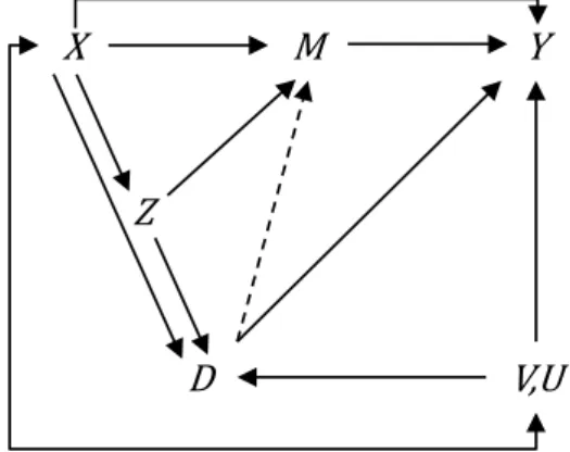
This section discusses cases in which conditioning on both 𝑀𝑀 and 𝑋𝑋 is necessary for (4) to hold. In Figure 4 we relax assumptions (i) and (iii) of Section 4.1: 𝑋𝑋 directly affects the outcome and is associated with the unobservables, while the instrument 𝑍𝑍 influences 𝑀𝑀. This is a combination of the models discussed in Sections (4.2) and (4.3). In this model, causal effects are only identified when controlling for both 𝑀𝑀 and 𝑋𝑋: Since pre-treatment covariates are jointly associated with post-war outcomes and the unobservables, conditioning on 𝑋𝑋 is required in an equivalent manner as in Figure (2). At the same time, the exclusion restriction of the instrument is not satisfied, which requires controlling for 𝑀𝑀 (as in the previous section). As before, under 𝐶𝐶 = 𝑋𝑋, 𝑀𝑀 the total effect can be identified only if veteran status does not affect post-treatment covariates.

Figure 4: Causal diagrams satisfying conditional IV independence for 𝐶𝐶 = 𝑋𝑋, 𝑀𝑀

X M Y

V,U D

Z

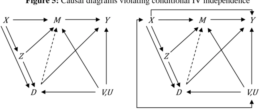
4.5 Conditional IV independence is violated

We now present several models in which the conditional IV independence assumption (4) is violated no matter which set of covariates serves as controls, so that identification is generally not obtained. This is the case if we relax assumptions (ii) and (iii) of Section 4.1 as in the left graph of Figure 5 or all three assumptions (i) to (iii), see the right graph of Figure 5. Because 𝑀𝑀 is also affected by 𝑍𝑍 (either directly or also indirectly via 𝐷𝐷), conditioning on 𝑀𝑀 introduces and association between Z and 𝑉𝑉, 𝑈𝑈. This introduces collider/selection bias as in section 4.2. However, not conditioning on 𝑀𝑀 does not satisfy (4) either, due to the causal path from the instrument to 𝑌𝑌 via 𝑀𝑀. It follows that neither the total, nor the direct effect are identified, no matter whether 𝐶𝐶 = 𝑋𝑋, 𝐶𝐶 = 𝑀𝑀, or 𝐶𝐶 = 𝑀𝑀, 𝑋𝑋.

Figure 5: Causal diagrams violating conditional IV independence

Unfortunately, such scenarios seem likely in many empirical problems where IV estimation is applied. With regard to the military draft, the educational deferment caused a strong incentive to be enrolled in college. Not controlling for education thus violates the exclusion restriction. However, education, labor market or health outcomes are the results of a common human capital investment process and are thus jointly determined. Since the underlying preference parameters are not fully observed in any conventional data source, education might be confounded by the same unobserved variables 𝑈𝑈, 𝑉𝑉.

X M Y V,U D Z X M Y V,U D Z 20

4.6 Summary of suitable conditional IV strategies

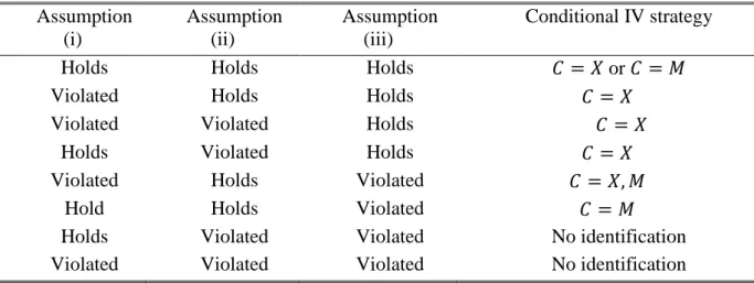
The previous sections presented alternative IV models and forms of conditional IV independence. We identified three crucial assumptions whose (non-)satisfaction determines the feasibility of conditional IV strategies based on various sets of control variables: (i) pre-treatment covariates 𝑋𝑋 have no direct effect on the outcome and are not associated with the unobservables in the outcome equation, (ii) post-treatment covariates 𝑀𝑀 are unconfounded, and (iii) the instrument 𝑍𝑍 affects any other variable only through the treatment of interest 𝐷𝐷. Table 1 summarizes our results on suitable identification strategies under the satisfaction/violation of some/all of these assumptions in our models.

Table 1: Feasible conditional IV strategies Assumption (i) Assumption (ii) Assumption (iii) Conditional IV strategy

Holds Holds Holds 𝐶𝐶 = 𝑋𝑋 or 𝐶𝐶 = 𝑀𝑀

Violated Holds Holds 𝐶𝐶 = 𝑋𝑋

Violated Violated Holds 𝐶𝐶 = 𝑋𝑋

Holds Violated Holds 𝐶𝐶 = 𝑋𝑋

Violated Holds Violated 𝐶𝐶 = 𝑋𝑋, 𝑀𝑀

Hold Holds Violated 𝐶𝐶 = 𝑀𝑀

Holds Violated Violated No identification

Violated Violated Violated No identification

We used the Vietnam draft risk instrument as an illustrative example to guide our discussion and suspect that no causal effect can be identified when using draft risk either as an instrument for veteran status or for college education. This was acknowledged by several authors, who therefore attempt to instrument both education and veteran status at the same time. Angrist and Krueger (1992), for example, transform draft risk into several categories and instrument both endogenous variables with these categories. Malamud and Wozniak (2010) compute national and state level draft risks and use them as separate instruments. In both applications, however, the constructed instruments essentially come from one single

phenomenon, namely draft risk, so that identification is delivered by functional form assumptions (which would not work in a completely flexible, nonparametric framework). An exception is Chaudhuri and Rose (2009), who use draft numbers as instrument for veteran status along with some additional instruments for education (i.e. the presence of a public or private four years college close the place of residence). In many applications, however, having available two or more instruments may be unrealistic. Finding just one valid and strong instrument is hard enough, as demonstrated in this paper.

5 Empirical application

In the following we use a publicly available data set to mimic previous conditional IV estimation strategies that use the Vietnam draft as exogenous variation and demonstrate that these strategies most likely yield biased results.

5.1 Data

Our data come from the “Young Men in High School and Beyond” (YESB) survey (Bachman, 1999), a five-wave longitudinal study among a national sample of male students who were in 10th grade in fall 1966. Information was collected in 1966, spring 1968 (at the end of eleventh grade), spring 1969, June-July 1970, and spring 1974. We make use of the first, fourth and last wave. This data set is particularly suited for studying the consequences of the draft lottery and potential draft avoiding behavior for three reasons: (1) More than 60% of the initial sample of 1966 were born in 1951 (1’380 respondents), the cohort exposed to the draft lottery of 1970. (2) It is to the best of our knowledge the only publicly available data set that provides the exact birth date for at least a subsample of respondents, which is necessary to link draft lottery numbers (available from the Selective Service System:

https://www.sss.gov/lotter1.htm) to individuals. (3) The data base also includes individuals

serving in the military (if they can be located).

Note that the exact day of birth is provided in the fourth wave (1970) for roughly two thirds of the initial sample, namely those individuals participating in the fourth wave and not serving in the military at the time of the interview (due to confidentiality reasons). Outcome variables are measured in wave 5 (1974) and subject to panel attrition, too. Of the 992 individuals born in 1951 with birth dates observed in wave 4, 104 dropped out in wave 5. Therefore, our final estimation sample consists of 888 individuals. Details on the sample definition are reported in the appendix (Table A1).

5.2 Using draft risk as instrumental variable

In this section we mimic strategies from the previous literature that exploits draft risk (either the lottery number, indicators for draft numbers below the ceiling, or broader aggregates such as the yearly induction risk) as an instrumental variable to estimate causal effects on various labor market and health outcomes. This literature can be classified into two different types: First, draft risk is used as instrument for veteran status (e.g., Angrist J. D., 1990; Angrist & Chen, 2011; Angrist, Chen, & Frandsen, 2010; Conley & Heerwig, 2011; Dobkin & Shabani, 2009), which usually assume that draft avoiding behavior is irrelevant. The second strand of literature explicitly takes draft avoiding behavior into account, namely by staying in/going to college and asking for a deferment. Draft risk is thus used as an instrument for education, while several researchers additionally control for veteran status to block the causal path that goes from having served in the army to the chosen outcome (e.g., Angrist & Krueger, 1992; de Walque, 2007; Grimard & Parent, 2007; Malamud & Wozniak, 2010).

Assume we would like to estimate the following (linear) outcome model: 𝑌𝑌 = 𝐷𝐷𝛽𝛽𝐷𝐷+ 𝐶𝐶′𝛽𝛽𝐶𝐶+ 𝑈𝑈,

where 𝑌𝑌 is the outcome of interest, 𝐷𝐷 is the treatment, either veteran status or education, and 𝐶𝐶 is a set of control variables including a constant. Most studies do not use longitudinal

data that allow conditioning on pre-treatment variables. They usually control only for time of birth, state of birth, or race and we mimic these strategies by only including month of birth and race in 𝐶𝐶. Moreover, we include veteran status – if not defined as treatment – as further control variable whenever we estimate the effect of education. 𝑈𝑈 is the unobserved term. 𝛽𝛽_𝐷𝐷 is the treatment effect of interest, 𝛽𝛽_𝐶𝐶 denotes the coefficients on the controls. We employ two stage least squares (TSLS), which is most frequent IV method in the literature, and estimate the following model of the supposedly endogenous treatment in the first stage:

𝐷𝐷 = 𝑍𝑍𝛼𝛼𝑍𝑍+ 𝐶𝐶′𝛼𝛼𝐶𝐶+ 𝑉𝑉.

𝑍𝑍 denotes draft risk, which is defined as an indicator that the draft number is below the ceiling of 125 (i.e. the maximum random lottery number drafted in 1971), 𝛼𝛼_𝑍𝑍, 𝛼𝛼_𝐶𝐶 are the coefficients, and 𝑉𝑉 is the unobserved term that may be arbitrarily correlated with 𝑈𝑈. The appendix also provides the results for IV probit regressions for binary outcomes, and 2SLS regressions for log incomes, in order to investigate the robustness of the results to deviations from the linearity assumption.

5.2.1 Instrumenting veteran status

The results of the first stage regression of the instrument on veteran status (reported in wave 5) are presented in the appendix (Table A2). The instrument is strongly associated with veteran status. Conditional on month of birth and race, individuals with low draft numbers are 22 percentage points more likely to have ever joined the army (F-statistic=99.55). The effect estimates of veteran status on various outcomes (unemployment, income, work disability) are provided in Table 2, where the first column presents the results from standard OLS and the second column those from 2SLS. The OLS estimates suggest that veterans have a somewhat higher probability to be unemployed, but are not statistically significant. 2SLS using the incidence of a draft number below the ceiling as instrument yields a higher effect of 11 percentage points which is significant at the 10% level. Given the overall unemployment rate

of only 4.4% in our sample, this is a sizeable effect. It is, however, unlikely persistent. Angrist and Chen (2011), for example, use a similar estimator and find no effects on unemployment in 2000.

Table 2: Effect of veteran status on labor market and health outcomes

OLS 2SLS Unemployment 0.02 0.11* (0.02) (0.07) Income (1973) 234 -3029** (410) (1334) Work disability -0.00 0.07 (0.03) (0.09)

Note: OLS/2SLS coefficients on veteran status for the sample of

individuals whose draft number is observed and who participated in the fifth wave (1974). The instrument for veteran status is a dummy indicating that the draft number was below the ceiling of 125. Control variables are month of birth and race. Standard errors are in parentheses. Significance levels: *** 1%; ** 5%; * 10%.

Information on incomes is retrospectively provided in brackets for the year 1973. We impute incomes by using bracket midpoints. Veterans report slightly (and insignificantly so) higher incomes compared to individuals who never served in the army. However, 2SLS suggests a very strong negative effect of draft-induced veteran status on incomes (-3029 USD compared to average income in our sample of only 5773 USD). This effect is larger than the ones published in the literature for subsequent time periods: Angrist (1990) documents that in the early 1980s, white veterans suffered an annual earnings loss of roughly $2000 (constant 1978) dollars (in relative terms this corresponds to a 15% decline in incomes). The veteran penalty in incomes shrinks until the beginning of the 2000s and is no longer statistical significant (Angrist & Chen, 2011).

OLS does not suggest large differences between veterans and individuals who never served the army in terms of self-reported work disability. In contrast, the 2SLS coefficient is positive

and relatively large, but very imprecisely estimated. Also Angrist, Chen and Frandsen (2010) analyze the impact of veteran status on health outcomes. They find that military service sharply increased federal transfer incomes (particularly veterans’ disability compensation), but had only a small impact on self-reported disability rates and no impact on work-limiting disability (i.e. health conditions that make work difficult).

5.2.2 Instrumenting education

In this section we present the results when using draft risk as an instrument for education (more precisely for the years of schooling), rather than veteran status. To “block” the causal path on outcomes arising from military service, we control for veteran status (as well as for month of birth and race). First stage regressions are provided in the appendix (Table A2, second column) and document that conditional on veteran status, individuals with draft numbers below 125 have 0.48 more years of schooling, which is statistically significant. The main estimates are given in Table 3.

Table 3: Effect of years on schooling on labor market and health outcomes

Note: OLS/2SLS coefficients on years of schooling for the

sample of individuals whose draft number is observed and who participated in the fifth wave (1974). The instrument for years of schooling is a dummy indicating that the draft number was below the ceiling of 125. Control variables are veteran status, month of birth and race. Standard errors are in parentheses. Significance levels: *** 1%; ** 5%; * 10%.

Both OLS (first column) and 2SLS (second column) yield insignificant effects of education on unemployment and health. Note, however, that the sign of the coefficients change and are

OLS 2SLS Unemployment -0.00 0.06 (0.00) (0.04) Income (1973) -998*** -1828*** (66) (656) Work disability -0.00 0.04 (0.01) (0.05) 26

unintuitive for 2SLS: one year extra of schooling increases unemployment by 6 percentage points and increases the likelihood of a work disability by 4 percentage points.

OLS results on income suggest lower incomes for more years of schooling. This is likely to be reflected by the fact that many respondents were still in school in 1973. The 2SLS coefficient is even larger and stands in stark contrast to previous estimates in the literature. Using a very similar approach with years in which schooling was likely completed (1979-1985) suggests that one extra year of schooling acquired in response to the lottery is associated with almost 7 percent higher weekly earnings, which is about 10% higher than the one achieved by a standard OLS regression (Angrist & Krueger, 1992).

5.3 Validity of the estimation strategies

As outlined in the section 4, the validity of the first conditional IV strategy estimating the effect of veteran status crucially relies on the assumption that no other confounding variables are jointly associated with draft-risk and the outcome and that draft-risk affects only veteran status but no other variable that also influences the outcome (exclusion restriction), which in our case may be violated by the education decision. The conditional IV strategy using draft risk as instrument for education, on the other hand, relaxes the exclusion restriction as it allows for an effect on veteran status, but requires controlling for the latter and all relevant confounders that jointly determine education, veteran status and outcomes. This rules out the endogeneity of veteran status (at least conditional on other observables), see Section 4.5. In the following, we provide empirical evidence for a violation of these assumptions.

5.3.1 Confounding pre-treatment variables

Even though the draft number is the result of a randomized lottery in 1970 that seems to be well executed (in contrast to the lottery held in 1969 where capsules were inadequately mixed and men with birthdates at the end of the year were more likely assigned low draft numbers),

the experiment may be broken due to sample selection, because we do not observe the draft number for the full sample. As mentioned before, the exact day of birth is provided in the fourth wave (1970) only for respondents in that wave that did not serve in the military at the time of the interview. Moreover, the outcomes measured in wave 5 (1974) are subject to further panel attrition. We thus have three different selection steps: (1) Panel attrition from wave 1 to wave 4; (2) military service that started before the interview in wave 4 took place; and (3) panel attrition from wave 4 to wave 5.

The first two selection steps are associated with individual background variables (such as cognitive skills and preferences) but are unlikely to be associated with the draft number:8 Young men born in 1951 were called to report for induction into the military in year 1971. Consequently, no individual of the initial sample was drafted when the interviews for the fourth wave took place. Moreover, most individuals were interviewed even before the lottery so that they were not aware of their draft number and could not have taken any steps to reduce the risk imposed by a small draft number (such as leaving the country). Therefore, the lottery should be internally valid (exogenous) for the individuals observed in 1971. However, the last selection step (drop out in wave 5) is more likely to be worrisome since we lose a further 10% of our subsample after the lottery. One would expect that dropout rates are highest among those with a high draft risk due to death on active duty, the inability to locate individuals who are still on active duty or draft avoidance by leaving the country. Surprisingly, this is not the case. Dropout rates are 2 percentage points lower for individuals with lottery numbers below 125 (9% vs. 11%). Moreover, if we restrict our sample to those still observed in 1974, differences in background variables are in most cases relatively small, not significant, and do

8 _{We do not observe any selective pattern in the distribution of lottery numbers for individuals who are observed}

in the 4th wave and there is no important and in most cases insignificant correlation between draft lottery numbers and background variables taken from the first wave (results are not reported but available from the authors upon request).

28

not seem to be systematic (results are not reported but available from the authors upon request).

We perform a series of sensitivity checks to analyze the robustness of the results presented in Table 2 with respect to omitted control variables. To this end, we randomly select ten potential controls and add them to the (baseline) 2SLS regression that estimates the effect of veteran status using draft risk as instrument.9 Since there is considerable missingness in the controls and regressions are only run in samples without missing information, we also re-estimate the baseline 2SLS model of Table 2 that does not include the additional confounders in exactly the same samples to guarantee comparability. This procedure is repeated 10,000 times.

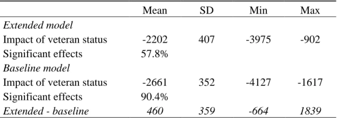
Table 4: Summary statistics of the sensitivity analysis

Mean SD Min Max

Extended model

Impact of veteran status -2202 407 -3975 -902 Significant effects 57.8%

Baseline model

Impact of veteran status -2661 352 -4127 -1617 Significant effects 90.4%

Extended - baseline 460 359 -664 1839

Note: Summary statistics from our 10,000 sensitivity checks, where the extended models

consist of the 2SLS model of Table 2 plus 10 randomly selected control variables. The

baseline models are specified as in Table 2, but are estimated in the same samples as the

extended models. Significant effects give the share of p-values of coefficients on veteran status that are smaller than 10% in the sensitivity checks. The last line presents summary statistics for the difference of coefficients on veteran status between the extended and baseline models.

9

Four waves of interviews took place before respondents were at risk to be drafted. In total, the survey contains more than 4000 potential control variables. We restrict our analysis to the first and fourth wave, and select information on families’ background and education (from wave 1) and on non-cognitive skills, values, and believes from questions that were administered to all individuals in wave 4. Moreover, we only focus on indices rather than on individual items. This results in 52 potential control variables. The full list can be obtained from the authors upon request.

29

The results of these sensitivity checks with income as outcome are summarized in Table 4.10 Adding control variables reduces the income penalty of veteran status by an average of 460 USD, suggesting that the veteran penalty may be overestimated in IV models as they are standard in the literature. Concerning the sign of the effect, we observe negative impacts of veteran status on incomes in all sensitivity checks. Interestingly, adding controls does not yield more precise estimates. Significant (negative) effects on incomes are found in 90% of the baseline models, but only in 58% of the extended models. The sensitivity analysis thus suggests that results are robust in sign but often not in significance or size.

5.3.2 Draft avoiding behavior

Another threat to the validity of the results presented in Table 2 is draft avoiding behavior. College deferments were issued until 1971, and about half of sample reported that they had already received a college deferment by the timing of the lottery. It was previously argued that the draft risk induced college enrollment (either by inducing new enrollments or preventing dropouts) among individuals at high risk. Card and Lemieux (2001) find a strong correlation between the risk of induction faced by a cohort and the male-to-female ratio in college enrollment and completed schooling, which however flattens out for cohorts born after 1950. In contrast, Angrist and Chen (2011) argue that the stark education premiums for individuals with low draft numbers (as observed in the 2000 census) were induced by the GI bill that finances continuous education after serving the military. Both arguments seem equally plausible at first glance, but have different implications for the validity of the instrumental variable strategy. Draft avoiding behavior violates (without further action) the exclusion restriction (as discussed in Sections 4.3 to 4.5), while military induced education does not and allows identifying the total effect of veteran status (i.e. the direct effect of veteran status and the indirect effect which works through post-service education).

10 _{We perform a similar analysis for the remaining outcome variables. Here we detect no large differences}

between the extended and the baseline models. Results are not presented but available from the authors. 30

Kuziemko (2010) considers the same data as we do to estimate the effect of the 1969 draft lottery on college attendance in 1970, focusing on young men born 1950 and before. She finds that a low lottery number immediately increases college attendance among whites, but decreases it among black and low-income men, providing support for the view that the lottery affects short term educational decisions which violate the exclusion restriction. Her analysis may be, however, constrained by the fact that at the timing of the interview, many young men have already been drafted or enlisted due to low draft numbers (consequently, draft numbers are not observed).

Table 5: Completed education (1974)

RDN > 125 RDN ≤ 125 Diff

Total years of schooling 14.34 14.46 0.12

Highest degree: high school or less 0.56 0.49 -0.07** Highest degree: associate's degree 0.10 0.15 0.05**

Highest degree: bachelor + 0.32 0.33 0.01

Note: The sample includes individuals whose draft number is observed and who participated in the fifth wave

(1974). Significance levels for the tests of equality in mean education outcomes: *** 1%; ** 5%; * 10%.

In our sample of individuals born in 1951 we cannot test for immediate educational reactions since no interview was conducted between 1970 and 1974. We, however, observe large and significant differences in completed education in 1974 (table 5). Individuals with low draft numbers are seven percentage points less likely to have at most a high school degree and five percentage points more likely to hold an associate’s degree. Given that (1) veterans reported that they served for 36 months on average, (2) no one in the sample started duty before summer 1970 (the large majority started military service in 1971), and (3) an associate’s degree takes two years of full time studying, the college degree effects of individuals with low draft numbers cannot be induced by the GI bill. Therefore, they are most likely be driven by draft avoiding behavior, which generally biases IV estimation strategies using draft numbers as instrument for veteran status.

5.3.3 Collider bias

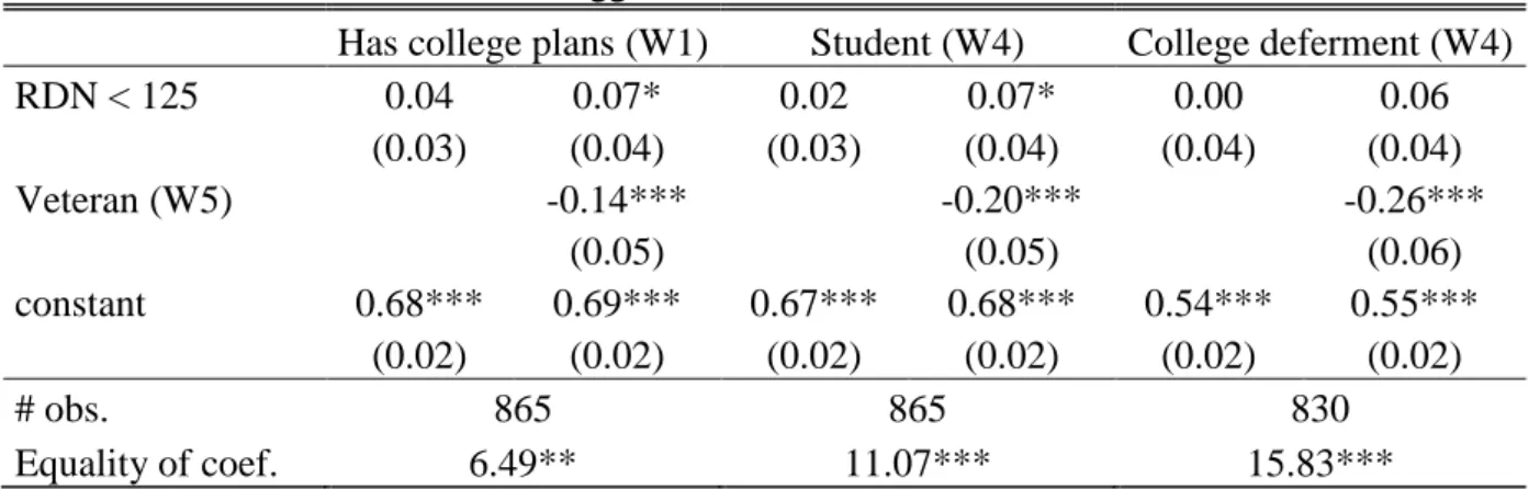
While the last section casts serious doubts on the IV validity when estimating the effect of veteran status, we subsequently also challenge the IV-based estimation of schooling effects. The key problem is the requirement to condition on veteran status, which on the one hand controls for direct effects (i.e., not going through education) of the lottery on the outcome, but on the other hand most likely introduces collider bias as outlined in Section 4.5, due to the potential endogeneity of veteran status. We observe that individuals with low aspirations to invest in formal education were particularly likely to join the army in case of a low draft number. For instance, respondents reporting to have a college deferment in 1970 were only 12 percentage points more likely to report being a veteran in 1974, while individuals without a college deferment were 33 percentage points more likely. Once we control for veteran status, individuals with low draft numbers contain a lower share of individuals with high educational aspirations, see Table 6. There, we regress three variables measuring the willingness to invest in education prior to drafting on the instrument or on both the latter and veteran status. When using the instrument as the only regressor, coefficients are small and insignificant. When additionally controlling for veteran status in wave 5, the coefficients on the instrument are substantially larger and in two out of three cases significant at the 10% level.

To demonstrate that collider bias matters, we add these measures of educational aspiration as further control variables in the 2SLS regression (results are presented in the appendix, Table A5). The “schooling penalty” in incomes increases from -1778 to a staggering -2621 USD. As both coefficients are estimated from exactly the same sample, the difference cannot steam from different sample definitions due to missing data. The prime reason for the increase in the penalty is the reduction in the instrument’s impact on total years of schooling (i.e., the first stage), which shrinks from a coefficient of 0.43 to 0.22 once we control for the measures of aspiration. While the true collider bias is of course unknown, this exercise documents how

sensitive conditional IV controlling for veteran status is w.r.t. the inclusion of a subset of potentially important confounders, which are usually not considered in the IV literature. Our 2SLS results among others suggest that collider bias induces an overestimation of the first stage effect of the lottery on education.

Table 6: Suggestive evidence for collider bias

Has college plans (W1) Student (W4) College deferment (W4) RDN < 125 0.04 0.07* 0.02 0.07* 0.00 0.06 (0.03) (0.04) (0.03) (0.04) (0.04) (0.04) Veteran (W5) -0.14*** -0.20*** -0.26*** (0.05) (0.05) (0.06) constant 0.68*** 0.69*** 0.67*** 0.68*** 0.54*** 0.55*** (0.02) (0.02) (0.02) (0.02) (0.02) (0.02) # obs. 865 865 830 Equality of coef. 6.49** 11.07*** 15.83***

Note: OLS coefficients on the draft number dummy, veteran status, and a constant when using various

background variables as outcomes (whether or not the respondent had plans to enroll in college in 1966, if the person was already student at the time of the interview in 1970, and if the person had a college deferment at the time of the interview in 1970). The sample includes individuals whose draft number is observed and who participated in the fifth wave (1974). Further control variables are veteran status, month of birth and race. Standard errors are in parentheses. Significance levels: *** 1%; ** 5%; * 10%.

6 Conclusion

This paper analyzed different conditional instrumental variable (IV) strategies controlling for observed covariates in a systematic way to understand under which conditions pre-instrument and/or post-treatment control variables are needed to achieve identification. For a rather general IV model where the instrument is not fully randomized but confounded by pre-instrument covariates, we identified three conditions that generally need to hold so that controlling for either pre-instrument or post-treatment covariates both yield causal effects: (i) Pre-instrument covariates have no direct effect on outcomes (other than through observed post-treatment covariates) and are not associated with the unobservables, (ii) post-treatment covariates are not confounded by unobservables, and (iii) the instrument does not directly affect any post-treatment variables (other than through the treatment of interest). However, if