T E C H N I C A L R E P O R T
Open Access
GEOMAGIA50.v3: 1. general structure and
modifications to the archeological and
volcanic database
Maxwell C Brown
1*, Fabio Donadini
2, Monika Korte
1, Andreas Nilsson
3,4, Kimmo Korhonen
5,
Alexandra Lodge
3,6, Stacey N Lengyel
7and Catherine G Constable
8Abstract
Background: GEOMAGIA50.v3 is a comprehensive online database providing access to published paleomagnetic, rock magnetic, and chronological data from a variety of materials that record Earth’s magnetic field over the past 50 ka. Findings: Since its original release in 2006, the structure and function of the database have been updated and a significant number of data have been added. Notable modifications are the following: (1) the inclusion of additional intensity, directional and metadata from archeological and volcanic materials and an improved documentation of radiocarbon dates; (2) a new data model to accommodate paleomagnetic, rock magnetic, and chronological data from lake and marine sediments; (3) a refinement of the geographic constraints in the archeomagnetic/volcanic query allowing selection of particular locations; (4) more flexible methodological and statistical constraints in the
archeomagnetic/volcanic query; (5) the calculation of predictions of the Holocene geomagnetic field from a series of time varying global field models; (6) searchable reference lists; and (7) an updated web interface. This paper describes general modifications to the database and specific aspects of the archeomagnetic and volcanic database. The reader is referred to a companion publication for a description of the sediment database.
Conclusions: The archeomagnetic and volcanic part of GEOMAGIA50.v3 currently contains 14,645 data (declination, inclination, and paleointensity) from 461 studies published between 1959 and 2014. We review the paleomagnetic methods used to obtain these data and discuss applications of the data within the database. The database continues to expand as legacy data are added and new studies published. The web-based interface can be found at http:// geomagia.gfz-potsdam.de.
Keywords: Geomagnetism; Paleomagnetism; Archeomagnetism; Database; GEOMAGIA50
Findings Introduction
Databases are a vital component of the global infras-tructure of science. In addition to ensuring the longevity of data, they enable the investigation of scientific ideas beyond those envisaged in the study for which the data were originally obtained. Furthermore, they encourage discourse on scientific standards, promote transparency in reporting on research, and ensure an ongoing return from publicly funded projects. Modern databases serve as
*Correspondence: [email protected]
1GFZ German Research Centre for Geosciences, Telegrafenberg, 14473 Potsdam, Germany
Full list of author information is available at the end of the article
digital libraries for research, with data archived at multi-ple levels and sophisticated search and analysis tools that allow users to find, visualize, and analyze a greater amount of data than ever before.
In paleomagnetic research there is a significant his-tory of compiling published data stemming from the early paleomagnetic pole lists (e.g., Irving (1959)) and the first paleointensity lists (e.g., Smith (1967)), which provided minimal printed summaries of important results at the time. These continually updated lists acknowledged the significant effort in acquiring data, including the reality that it is not always possible to repeat field or exper-imental work, and allowed future generations to build new interpretations that took into account pre-existing © 2015 Brown et al. This is an Open Access article distributed under the terms of the Creative Commons Attribution License (http://creativecommons.org/licenses/by/4.0), which permits unrestricted use, distribution, and reproduction in any medium, provided the original work is properly credited.
results. The same advantages apply to more modern pale-omagnetic and rock magnetic data compilations based on relational databases (beginning with the IAGA Global Paleomagnetic Database (GPMDB), Lock and McElhinny 1991; McElhinny and Lock 1996; Pisarevsky 2005) that have now evolved the potential to store highly detailed information ranging from raw field and laboratory mea-surements through multiple processing steps to results (e.g., MagIC, Constable et al. (2006); Jarboe et al. (2012)).
The aim of the GEOMAGIA50 database is to provide easy access to the significant amount of paleomagnetic, rock magnetic, and chronological data covering the past 50 ka that have been obtained from archeological mate-rials, volcanic rocks, and sediments. These data have a range of applications within geosciences. Determining the temporal and spatial evolution of the geomagnetic field improves our understanding of the geodynamo and deep Earth processes; geomagnetic shielding against solar wind and galactic cosmic rays; the modulation of cosmo-genic radionuclide production; and interactions between the geomagnetic field and climate. Robustly constrained temporal variations in the geomagnetic field can be used to date the time of firing of archeological materials, the emplacement of lavas, or the deposition of sediments. Fur-thermore, variations in the rock magnetic properties of sediments can reflect changes in environment, climate, and anthropogenic impact. Greater detail on the appli-cations of data within GEOMAGIA50 are described in the ‘Applications of archeomagnetic and vol canic data from GEOMAGIA50’ section and a companion paper (Brown et al. 2015), which describes the substantial mod-ifications made to the database to include sediment data.
GEOMAGIA50 originally began in 2006 as a database of global field intensity data from archeological and vol-canic materials (Donadini et al. 2006; Korhonen et al. 2008). It built upon previous efforts to catalogue archeo-magnetic and recent paleoarcheo-magnetic results, on paper (e.g., Eighmy and Sternberg 1990; Smith 1967), as regional or global compilations (see the ‘Archeological and volcanic data sources’ section), or in digital databases (Liritzis and Lagios 1993; Perrin and Schnepp 2004; Sternberg et al. 1997; Tarling and Dobson 1995).
GEOMAGIA50 employs the philosophies of a
Rela-tional Database Management System (Codd 1970) and uses Standard Query Language (SQL), the official international language for database management sys-tems, as recognized by the International Organization for Standardization (ISO). These principles underlie the IAGA paleomagnetic databases (e.g., Lock and McEl-hinny (1991)) and have been applied successfully in more recent paleomagnetic databases, MagIC (Constable et al. 2006) and PALEOMAGIA (Veikkolainen et al. 2014). Since 2008, GEOMAGIA50 has been queried 10,264 times
(approximately 1,700 queries per year) and Donadini et al. (2006) and Korhonen et al. (2008) have 53 unique citations between them.
This paper and its companion (Brown et al. 2015) address updates and extensions to the most recent version of the GEOMAGIA50 database and web portal (GEO-MAGIA50.v3). The first version of the database provided convenient access not only to intensity data spanning ages of 0 to 50 ka, but also included a wealth of infor-mation about any associated paleomagnetic directions, experimental and dating methods, materials, number of samples measured, and other metadata (see Korhonen et al. (2008)). A recognition of issues concerning the fidelity of archeological materials and lavas to accurately record the intensity of the geomagnetic field led to the inclusion of detailed metadata on paleointensity methods. Constable and Korte (2015) and Donadini et al. (2010) give recent overviews of data types and experimental methods employed to gain magnetic field information from archeo-logical material, lavas and sediments, in particular for the Holocene epoch.
Since the release of the first version of GEOMAGIA50, a continued interest in improving global spherical har-monic models of the Holocene geomagnetic field, initi-ated by the work of Constable et al. (2000) and Korte and Constable (2003), triggered a desire to include more comprehensive directional data from archeological and volcanic materials in an updated version of the database (GEOMAGIA50.v2). Concurrently, the production of new archeomagnetic data strongly increased as a result of the European AARCH project (2002 to 2006) (Figure 1), which aimed to improve European regional reference curves for geomagnetic dating of archeological materials (e.g., Gómez-Paccard et al. (2006a); Márton and Ferencz (2006); Schnepp and Lanos (2006); Tema et al. (2006); Zananiri et al. (2007)). In June 2008, archeo/volcanic directions and intensity data with increased metadata were made accessible through an updated data model in GEOMAGIA50.v2 (http://geomagia.ucsd.edu.), which included global data sets compiled for specific modeling purposes (Constable et al. 2000; Korte et al. 2005; Genevey et al. 2008; Donadini et al. 2009) and incorporated data from the AARCH project. At this time, it was also envis-aged that future modifications would allow incorporation of sediment records; however, this was not realized until GEOMAGIA50.v3 (see Brown et al. 2015).
In addition, the importance of equatorial and southern hemisphere data has been recognized for global mod-eling (e.g., Korte and Constable (2005)) and for under-standing the evolution of the South Atlantic anomaly (e.g., Mandea et al. (2007)). This has driven recent efforts to obtain archeomagnetic data from Argentina (Goguitchaichvili et al. 2010, 2011), Brazil (Hartmann et al. 2010, 2011), India (Venkatachalapathy et al. 2013),
1960 1970 1980 1990 2000 2010 0 5 10 15 20 25 Publication Year Number
Figure 1 Number of archeomagnetic and volcanic studies published per year included in GEOMAGIA50.v3.
Senegal and Mali (Mitra et al. 2013), South Africa (Neukirch et al. 2012), and the SW Pacific (Stark et al. 2010). Furthermore, determining the age of magnetiza-tion is a major challenge; however, the quality of the age determination is crucial, e.g., when interpreting tem-poral variations in regionally compiled archeomagnetic curves (e.g., De Marco et al. (2008); Hagstrum and Blinman (2010); Márton (2010); Shaar et al. (2011); Tema and Kondopoulou (2011)) or in comparing magnetic field variations in sediment records from different locations (e.g., Nilsson et al. (2010, 2014)). This has led to the expan-sion of the chronological metadata included in the latest version of the database.
In parallel with the development of GEOMAGIA50, databases under the Magnetics Information Consortium (MagIC; Constable et al. (2006)) have undergone sys-tematic evolution from a somewhat different perspective. MagIC (started in 2003) intends to capture as much data and associated metadata as possible throughout the work flow from field and/or lab work to analysis and eventual publication. In contrast, the simpler structure and web query interface provided by GEOMAGIA50 provides a straightforward way to recover selected but extremely useful results with specific attributes from identified locations and age ranges. MagIC also accepts these more limited data sets, and since 2007, the col-laborative intent has been to share information between GEOMAGIA50 and MagIC, so that effort expended in populating one database does not need to be duplicated later.
This paper begins by describing what we see as the major successes and future applications of the database (‘Applications of archeomagnetic and volcanic
data from GEOMAGIA50’ section). This is followed by the principles behind the database (‘Principles of the GEOMAGIA50.v3 database’ section), the general ture and function of the updated database (‘General struc-ture of the MySQL database’ section), documentation of the data types stored within GEOMAGIA50.v3 (‘Archeo-logical and volcanic data types’ section), and the sources of the data (‘Archeological and volcanic data sources’ section). A summary of the key changes between GEO-MAGIA50.v1 and GEOMAGIA50.v3 is given in the ‘Mod-ifications and updates to the archeomagnetic and volcanic database’ section. Although version 2 data were described in part in Donadini et al. (2009), no comprehensive pub-lication described the data model and the web-based user query form of GEOMAGIA50.v2. We remedy this by doc-umenting the update of the database to GEOMAGI50 .v3, which has been expanded to accommodate sedimen-tary paleomagnetic, rock magnetic, and geochronological data (see Brown et al. (2015)), in addition to a wider range of results from archeological and volcanic mate-rials (‘Modifications and updates to the archeomagnetic and volcanic database’ section). We note in particular the inclusion of a greater number of archeomagnetic and vol-canic directional data, more extensive chronological data and additional metadata, as well as modifications to the user interface that allow more refined data searches, the calculation and plotting of geomagnetic field model pre-dictions, and visualization of data locations within Google Earth.
The ‘User interface: GEOMAGIA50.v3 web page’ section describes the rationale behind the web-based archeomagnetic/volcanic query form. Finally, Additional file 1 contains a user guide to the archeomagnetic/volcanic
query form and a description of the global Holocene geo-magnetic field models that can be queried through the database interface.
The database is maintained in mirror versions on servers at the German Research Centre for Geo-sciences GFZ in Potsdam, Germany (http://geomagia.gfz-potsdam.de), and at the University of California at San Diego, USA (http://geomagia.ucsd.edu/).
Applications of archeomagnetic and volcanic data from GEOMAGIA50
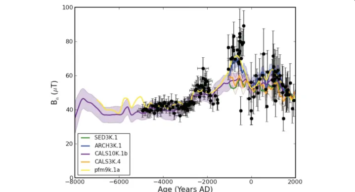
Data from GEOMAGIA50 have been used in studies of geomagnetism, the deep Earth, the space environment, climate, volcanism, and archeology. A particularly notable use has been in the creation of temporally continuous models of the global Holocene geomagnetic field (e.g., Korte et al. (2009, 2011); Licht et al. (2013); Nilsson et al. (2014); Panovska et al. (2015); Pavón-Carrasco et al. (2014a)) and regional models of the geomagnetic field (Pavón-Carrasco et al. 2010; Pavón-Carrasco et al. 2014b), for which data from GEOMAGIA50 are a vital component. These models allow mapping of changes in the geomagnetic field at Earth’s surface and core-mantle boundary through time, placing constraints on the evolu-tion of the past geomagnetic field.
As global field models are constructed to recreate the field at the core-mantle boundary, they have the poten-tial to be used to understand the geodynamo and have been used to investigate core flow (Dumberry and Finlay 2007; Wardinski and Korte 2008; Livermore et al. 2014), with possible implications for length of day variations on millennial time scales (Dumberry and Bloxham 2006); the behavior of high latitude flux patches (Korte and Holme 2010; Amit et al. 2011); hemispheric field asymme-tries related to archeomagnetic jerks (Gallet et al. 2009); discrete scale invariance across geodynamo time scales (Jonkers 2007); and similarities with the characteristics of dynamo simulations (Christensen et al. 2011; Heimpel and Evans 2013; Davies and Constable 2014). Calcula-tions of dipole eccentricity using CALS3k.4b (Korte and Constable 2011) and CALS10k.1b (Korte et al. 2011), coupled with observations of hemispherical variations in seismic velocity at the top of the Earth’s inner core, motivated Olson and Deguen (2012) to investigate per-sistent eccentricity in numerical dynamo simulations and they suggested lopsided solidification within the inner core. Brown et al. (2007), Valet and Plenier (2008), Valet et al. (2008), and Valet et al. (2012) investigated surface field morphologies and statistical characteristics of the field during simulated reversals and excursions by using CALS7K.2 (Korte and Constable 2005) and CALS10k.1b (Korte et al. 2011) and imposing changes on the axial dipole component of the field while leaving the non-dipole field unchanged.
Studies of cosmogenic radionuclide production (e.g.,
14C, 10Be, 36Cl, and 3He) in Earth’s atmosphere have
employed estimates of dipole strength from the CAL-Sxk series of models to calibrate variations in production activity (e.g., Kovaltsov et al. (2012); Lifton et al. (2014); Schimmelpfennig et al. (2011)). Production rates have then been used to calculate past solar activity (Delaygue and Bard 2011; Snowball and Muscheler 2007; Usoskin et al. 2006) and surface exposure ages (Lifton et al. 2008; Balco et al. 2008). Similarly, studies of cosmic ray ion-ization in the troposphere (Usoskin et al. 2008, 2010) and theoretical models of the inner proton radiation belt (Selesnick et al. 2007) have incorporated geomagnetic constraints from CALS7K.2. Geomagnetic field models have also been used to estimate the occurrences of aurora at mid-latitudes in the Northern Hemisphere over the past 10 ka (Korte and Stolze 2014).
When age control is uncertain in sediment and arche-ological studies, the time varying location dependent outputs of models have been compared with the paleo-magnetic field recorded in these materials. This has aided in understanding the timing of climate events recorded in sediments (e.g., Antoniades et al. (2011); Barletta et al. (2010); Ledu et al. (2010)) and the dating of archeologi-cal and volcanic materials (see Lodge and Holme (2009), Pavón-Carrasco et al. (2009), and Villasante-Marcos and Pavón-Carrasco (2014)). Models based on archeological data have been used to study the lock-in process in pre-cisely dated sediment sequences (Mellström et al. 2015).
In addition to global geomagnetic field modeling, arche-ological and volcanic data within GEOMAGIA50 can be used to investigate statistical characteristics of the geo-magnetic field (Donadini et al. 2007; Roberts et al. 2013); develop archeomagnetic reference curves (e.g., Fanjat et al. (2013); Hellio et al. (2014); Márton (2010); Tema and Kondopoulou (2011)), which aid in the dating of archeo-logical materials that form the backbone of archeoarcheo-logical studies; understand material and methodological bias in paleointensity estimates (Donadini et al. 2007); calculate mean dipole moments (Knudsen et al. 2008); and explore links between climate and the geomagnetic field (Knudsen and Riisager 2009).
Further applications of archeological and volcanic data from GEOMAGIA50 include dating of eruptive episodes through comparison of paleomagnetic directions and intensities recorded in lavas and volcanic deposits with reference curves (e.g., Di Chiara et al. (2014); Holcomb et al. (1986); Speranza et al. (2008)) (however, caution must be taken when relocating reference curves to erup-tion locaerup-tions when the distance between the two is large). Absolute paleointensity data can be used to cali-brate relative paleointensity (RPI) records from sediments (Donadini et al. 2009; Korte and Constable 2006) which can refine global models of the geomagnetic field and
improve global stacks of RPI (e.g., SINT2000 (Valet et al. 2005) and PISO-1500 (Channell et al. 2009)). Finally, pale-omagnetic data within GEOMAGIA50 have the potential to be incorporated in data assimilation strategies for mod-eling and forecasting the geomagnetic field (see Fournier et al. (2010); Kuang et al. (2008, 2009)).
Principles of the GEOMAGIA50.v3 database
The GEOMAGIA50 database is based upon the princi-ples of a Relational Database Management System (Codd 1970). Users access the data through a web-based inter-face. There are three primary components to the database design model (Figure 2):
1. The digital storage and management of the data; 2. The web-based interface (query forms and HTML
output);
3. Programming that transfers information back and forth between (1) and (2).
We employ the LAMP (Linux, Apache, MySQL, PHP) model of web service management to produce a dynamic web-based database for the user. All components of this model are open source.
Data are primarily stored and managed using the ORA-CLE MySQL database management system on a Linux-based server at the Helmholtz Centre, GFZ Potsdam.
volcanic Sediment Archeomagnetic Individual (specimen/stratigraphic) Processed (averaged/smoothed) Reconstructed Sediment database Country/ Region ID
Figure 2 A schematic of the general structure of the GEOMAGIA50.v3 database. The grey dot-dashed box contains relational tables (results and
metadata tables) housed within the ORACLE MySQL database. The grey short-dashed lines nominally divide the results tables between those which contain archeomagnetic and volcanic data and those containing sedimentary data. The long-dashed box contains the three parts of the web page visible to the user. Lines with arrow heads represent the two-way transfer of information between different parts of the database (e.g., query commands and data return). Orange represents archeomagnetic and volcanic commands and data transfer; blue = sediments. Solid black lines show the links between results tables annotated by the linking ID. The elements of the figure are explained further in the ‘Principles of the GEOMAGIA50.v3 database’ section.
The database is mirrored at the University of California, San Diego. The long-term availability of the database is secured through the commitment of both institutions. The relational nature of the MySQL database allows a col-lection of tables to be manipulated and joined using the SQL language. This avoids repetition of fields within dif-ferent tables as the information only needs to be entered once. In addition, it allows complex queries to be com-posed and data sets based upon multiple search criteria to be returned.
We chose to employ a web-based user interface, rather than an installation-based software such as for the IAGA databases (http://www.ngdc.noaa.gov/geomag/ paleo.shtml), as it has the following advantages:
1. No proprietary software are required by the user; 2. It requires only access to the internet and a web
browser;
3. It is platform independent (there are only minor differences whether run on Windows, Macintosh or Linux operating systems);
4. The data and metadata available to the user can be dynamically updated as new data become available, rather than a new software package being required; 5. It has global visibility as it is returned in web search
engines.
Requests are processed using an Apache HTTP web server. This allows us to implement server-side program-ming languages that handle requests from the web page and return data and plots from the server to the web page. We use the PHP (Hypertext Preprocessor) script-ing language to transform users’ data requests into query statements that can be read by the MySQL database. Java script is used to provide additional web page functionality. PHP is used to process the data recalled by the database into a series of HTML tables and .CSV files that can be viewed online and downloaded from the web page (see ‘Query results’ section).
Graphical output (‘Figures and downloads’ section) is generated by first processing the data recalled from the database in a PHP script. Plots are then created using the Python programming language, stored on the server, and recalled to the web page through further PHP scripting.
Site-dependent output of a series of Holocene geomag-netic field models (see Additional file 1) can be generated as a .TXT file (‘Query results’ section) and plotted along-side the data (‘Figures and downloads’ section). The mod-els are run using a series of Fortran routines. Again, the output is interpreted by the PHP coding and graphs are generated using Python.
The web pages are hosted at http://geomagia.gfz-potsdam.de/ and mirrored at http://geomagia.ucsd.edu/. The functionality of the web-based query form for the
archeomagnetic and volcanic database (http://geomagia. gfz-potsdam.de/geomagiav3/AAquery.php) is briefly des-cribed in ‘Querying the database: the ‘archeomagnetic and volcanic data’ query form’ section and in more detail in a user’s guide in Additional file 1. The sediment query form is described in Brown et al. (2015). In addition to the web-based query forms, web-pages have been designed to recall metadata from the database. These include search-able lists of archeo/volcanic and sediment studies (‘Web site features’ section) and a glossary of identification num-bers used to describe the metadata (‘General structure of the MySQL database’ section).
General structure of the MySQL database
GEOMAGIA50.v3 builds upon the database structure outlined in Korhonen et al. (2008) (herein referred to as K08). In this section we describe developments to the overall structure of the database and its main components. To aid this description, we have tabulated commonly ref-erenced terms (Table 1). A schematic diagram outlines the general structure of the database (Figure 2).
A key development between versions 2 and 3 of the database is the inclusion of sediment data and this has expanded the database structure significantly. Sediment data are collected, measured, processed, and analyzed in different ways to archeological and volcanic data. We have therefore developed a series of structurally distinct results and metadata tables to accommodate the differ-ent and varied parameters measured in sedimdiffer-ent studies. The structure of the sediment database and the content of the results tables are discussed thoroughly in Brown et al. (2015).
The version 3 database consists of two sets of results tables, those for the archeomagnetic and volcanic side of the database and those for the sediment side of the database (Figure 2). There are two archeomagnetic and volcanic results tables: a magnetic data results table and a radiocarbon age results table.
The magnetic data results table contains age (‘Chrono-logical data’ section), paleomagnetic results (‘Paleomag-netic data’ section), and a variety of metadata (‘Metadata’ section). The full list of fields is shown in Additional file 1: Table S1. All entries have an associated age and repre-sent data at the site level (as defined in Table 1). This is the most convenient option for presenting and analyzing time series of data. GEOMAGIA50 does not store sample or specimen paleomagnetic results (unless these are the only results available from a site) or rock magnetic data. It does not store the individual demagnetization or remagneti-zation steps used to determine a directional or intensity estimate of the geomagnetic field (see the ‘Paleomagnetic data’ section). In many cases, these data are not avail-able, unless obtained directly from the author of a study. Although the provision of rock magnetic data is important
Table 1 Glossary of terms employed in GEOMAGIA50
Term Description
Entry A row of information within a results or metadata table.
In database terminology this is often called a record; however, within sediment stud-ies, the use of record denotes a complete data set.
An entry shows data at the site level. Field A column of information within a result or
metadata table.
Identification number (ID) A number within a results table that links to an identical number (the primary key) within a metadata table, allowing the return of a description of the ID.
Location A geographical area with similar character-istics, smaller than a country/region, which can contain a number of sites, e.g., an archeological excavation or a volcano. Metadata table A two dimensional relational table
containing a primary key field and descriptive fields.
Primary key A number that links an entry or parts of an entry between relational tables.
Relational table A table that can be related to another by associations between tables and which can be joined using the SQL language. They negate repetition of fields between tables by employing primary keys, which allow values within one field to link to com-plete entries or parts of entries between tables.
Results and metadata tables are relational tables.
Results table A large two dimensional relational table with multiple fields and unlimited entries containing results and IDs.
Sample A portion of material obtained from a site, which can be subdivided into specimens, e.g., a fragment of a pot from which smaller parts were taken or a drill core from a lava. Specimen The smallest division of a material used to
determine a measurement, e.g., a piece of a pot fragment or a standard cylinder from a lava drill core.
Site A material/medium/stratum/geological unit which can be assigned a unique age, e.g., a pot, a layer at an archeological excavation or a lava flow.
to understanding the reliability of palaeomagnetic data, rock magnetic data are generally reported at the speci-men level and are therefore not easily accommodated in the current structure of the GEOMAGIA50 database. The MagIC database (Constable et al. 2006) has already devel-oped the necessary structures to accommodate specimen level paleomagnetic and rock magnetic data and is the most suitable place to store these data.
The radiocarbon age results table is a new addition in version 3 of the database. It has been designed to accom-modate experimental radiocarbon ages and their uncer-tainties at one standard deviation (see ‘Chronological data’ section). In addition, it shows the preferred ages and uncertainties of the author, the sample names used in a publication as well as the sample codes used by the radio-carbon dating facility (‘Chronological metadata’ section). The full list of fields are shown in Additional file 1: Table S2. The radiocarbon results table is associated with the magnetic data results table via an identification num-ber (ID) called ‘C14 ID’. This appears in the penultimate column of the magnetic data results table and is again found in the first column of the radiocarbon ages results table.
The sediment database contains five results tables (Figure 2). The content of the results tables and the rationale behind them is described in Brown et al. (2015). Every results table contains a country/region ID. This ID allows the tables to be joined within an MySQL statement when querying the database. This maximizes the efficiency of the relational table struc-ture and only one statement is required to return entries from all the results tables related to a specific query.
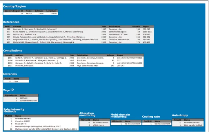
In addition to the archeo/volcanic and sediment results tables, 43 metadata tables contain specific information about, e.g., paleomagnetic experimental details, spec-imens types, and references (see http://geomagia.gfz-potsdam.de/ID_glossary.php for a list of tables). Metadata for the archeo/volcanic database are discussed in detail in the ‘Metadata’ section. Sediment metadata are dis-cussed in Brown et al. (2015). The use of metadata tables allows IDs to replace specific fields of metadata informa-tion within a results table. For example, each reference is assigned an ID. The metadata table will contain this ID (which acts as the primary key) followed by other fields for authors, year, journal, etc, (see Table ten, K08, for an example). Rather than the full reference being listed in a results table, only the reference ID is shown. When search criteria are specified by the user, a MySQL statement is constructed which joins the information within the results table and the metadata table and returns only references related to the specific query. Metadata tables can be used by both the archeo/volcanic and the sediment database, e.g., the country/region metadata table (http://geomagia. gfz-potsdam.de/ID_glossary.php#CRID) and by multiple fields within a results table. This reduces the number of metadata tables required. This is the case for many fields in the sediment database. For example, there are multiple dating fields related to different types of dating methods. For each dating method an age can be reported, but as the statistical methods used to calculate the ages are applica-ble to all dating methods, they can be grouped within one
metadata table. This one metadata table can then be called for all the dating types.
To aid the transparency of data reporting, every entry in the archeomagnetic and volcanic database is assigned a unique identification number (UID). UIDs will remain the same throughout the life of the database and indicate the order of the upload of entries through time, i.e., UID = 1 was the first entry uploaded to GEOMAGIA50.
A similar approach has been taken with the sedi-ment data; however, a more sophisticated scheme has evolved to cater for the five results tables and the much larger number of entries compared with the archeo-magnetic and volcanic database. The UIDs for the dif-ferent results tables follow the format: ABC-Xnnnnn, where ABC is the three letter location code of the sediment location (http://geomagia.gfz-potsdam.de/ID_ glossary.php#SedLocCode), X is replaced by an abbrevi-ation for the type of results table (C - individual (speci-men/stratigraphic); S - processed (averaged/smoothed); D - radiocarbon ages; A - general ages; R - reconstructed), and nnnnn is the number of the entry (up to 99999). For example the first entry in the Lake Keilambete individual (specimen/stratigraphic) results table is KEI-C00001.
UIDs have previously been used in Donadini et al. (2009) to denote specific entries that were excluded for the modeling of Korte et al. (2009). In contrast to previ-ous versions of the database they are now visible to the user. The UID allows the user to see the order of upload and quickly identify that an entry is unique when process-ing a large amount of data. If data from GEOMAGIA50 are used in future modeling efforts or in another form of analysis and certain data are excluded from the modeling or specific data require discussing, then the UID provides a brief and unambiguous way to communicate this infor-mation. Other users can use the UID to quickly relocate the data referred to in a publication within the database. In addition, if a user finds an error within an entry, this is the most efficient way to report a problem to a member of the database team.
Archeological and volcanic data types
The data within GEOMAGIA50 can be broadly classed into three types:
1. Paleomagnetic data; 2. Chronological data; 3. Metadata.
GEOMAGIA50.v1 and v2 contained the above data types from two categories of materials: archeological and volcanic (e.g., lavas, ash deposits, and pyroclas-tic deposits). GEOMAGIA50.v3 has been expanded to include paleomagnetic, rock magnetic, chronological, and metadata obtained from lake and marine sediments
deposited over the past 50 ka. These data are described fully in Brown et al. (2015). The following subsections focus solely on data acquired from archeological and vol-canic materials.
Paleomagnetic data
Archeological and volcanic materials have the poten-tial to acquire a natural remanent magnetization (NRM) that is thermal in origin (termed a thermal remanent magnetization or TRM). TRM is obtained on cooling through a material’s Curie-temperature (Néel tempera-ture) to room temperature and can be preserved over geological timescales depending on the magnetic grain size distribution of a particular material. A TRM can be treated as the summation of blocks of magnetization asso-ciated with discrete temperature ranges (called partial TRM or pTRM). In the laboratory it is possible to reverse the magnetization process (demagnetization). By repeat-edly heating a material carrying a TRM in a zero-field to increasing temperature steps, pTRMs can be demagne-tized and the magnetization history of the material can be recovered. After each temperature application, the mag-nitude of three orthogonal components of magnetization can be measured at room temperature. If the material records a direction representative of a spot reading of the geomagnetic field (without secondary contamination), the components of magnetization will linearly decrease to zero with increasing temperature and a characteristic remanent magnetization (ChRM) direction (represented as declination and inclination) can be calculated for a par-ticular temperature step or across a range of temperature steps.
As an alternative to heating, materials can be demag-netized by applying an alternating field (AF). Archeo-logical and volcanic materials may contain a range of magnetic grain sizes, which can be demagnetized with different alternating fields. In a similar approach to ther-mal demagnetization, an AF can be increased in steps and if the resulting magnetization at each increasing AF step decreases linearly to zero, a ChRM inclination and declination can be calculated.
As discussed in ‘General structure of the MySQL database’ section, paleomagnetic data within the database are reported at the site level, i.e., at a level where the magnetization recorded by a material/medium/stratum/ geological unit can be assigned a unique age. If more than one specimen was used to estimate the direction or pale-ointensity (see below) of a site, as is common, the data in this entry will be a mean. If a mean was reported in a publication, this value is included in the database. If a mean was not published, yet multiple specimen or sample data were available, then a mean was calculated following Fisher (1953) and this is the value reported in the database.
There is no method prerequisite for the mean direc-tional data included in the database. Mean directions are most commonly calculated from specimens demagnetized by thermal and AF methods, with specimen directions determined from either a single demagnetization to a certain temperature or AF step, or from a fit to step-wise demagnetization data, e.g., by principal component
analysis (Kirschvink 1980). Mean directions are frequently calculated using the statistics of Fisher (1953), however, mean directions calculated by any method are listed in the database. The distribution of inclination and declination data over the past 50 ka is shown in Figure 3.
In addition to recording the direction of the field, a TRM can preserve an intensity proportional to the past
(a) (b)
(c) (d)
(e) (f)
Figure 3 Distributions of archeological and volcanic data over the past 50 ka. (a-d) Data distribution through time in 500 year bins comparing
archeological and volcanic sources for (a) all data, (b) intensity, (c) inclination, and (d) declination. (e) Distribution ofα95in 1° bins and (f) intensity
uncertainties in 1μT bins. White bars show all data, light gray show archeological data only and dark gray show volcanic data only. The numbers of specific data types are noted on the graph labels. There are less data for the intensity uncertainties than for the intensities as not all intensity data has been reported with an associated uncertainty.
strength of the geomagnetic field (termed paleointensity). A variety of methods based upon different principles can be used to experimentally estimate paleointensity. See the ‘Paleointensity metadata’ section for a brief description of these methods as they relate to the paleointensity meta-data stored in the meta-database. See Valet (2003), Tauxe and Yamazaki (2007), and Dunlop (2011) for more detailed reviews of paleointensity methods. In brief, all paleointen-sity methods replace the NRM, either as a whole or in part, with a full TRM or pTRMs acquired in a known labora-tory field. Assuming the relationship between the strength of magnetization of the removed NRM and the acquired TRM is directly proportional to the ancient field divided by the laboratory field, the ancient field can be estimated by multiplying the ratio of NRM to TRM by the strength of the laboratory field.
In practice, there are a number of complicating factors that can make the relationship between NRM and TRM nonlinear and/or nonproportional to the ancient field. This can depend in part on the paleointensity method chosen. Such factors include the influence of multi-domain (MD) grains, thermal alteration during heating, acquisition of a thermochemical remanent magnetization (TCRM) on cooling in nature (e.g., Kellogg et al. 1970; Nagata and Kobayashi 1963; Yamamoto et al. 2003), differ-ences between cooling rates in nature and the laboratory, remanence anisotropy, and non-linear acquisition of TRM with increasing applied field (see Perrin et al. (1998); Valet (2003); Tauxe and Yamazaki (2007); Fabian and Leonhardt (2009) for overviews of the majority of these issues). These problems can result in ambiguity in interpreting paleoin-tensity experiments and may lead to significantly inac-curate estimates of paleointensity. A number of checks and/or corrections have been developed to address these issues, and the database accommodates metadata related to the most significant of these methods (‘Paleointensity metadata’ section).
Paleointensity estimates obtained using any paleoin-tensity method are listed in the database; however, only metadata from certain methods accompany these data (see the ‘Paleointensity metadata’ section). Mean paleoin-tensities can be statistically calculated in a variety of ways and these are not always clearly reported in the literature. Means may be arithmetic or weighted and several differ-ent weights can be applied (e.g., Coe et al. (1978); Prévot et al. (1985)). The reader is advised to check a spe-cific publication to determine the method used to cal-culate a mean. It is not currently documented in the database. If mean paleointensities were not calculated in a publication, then we calculated an arithmetic mean from the reported specimen or sample intensity and this is the value reported in the database. The distribu-tion of intensity data over the past 50 ka is shown in Figure 3.
In addition to paleointensity, corresponding values of virtual dipole moment (VDM) and virtual axial dipole moment (VADM) are accommodated in the database. As the intensity of the geomagnetic field, when in a dipole configuration, is latitude dependent, intensity val-ues obtained from different latitudes can not be com-pared easily. By assuming a dipolar structure, VDMs and VADMs allow comparison of global intensity values. A VADM has the equivalent moment of a magnetic dipole aligned with Earth’s rotation axis for a measured intensity at a given latitude (see equation (1) in K08). In com-parison, a VDM is calculated using magnetic colatitude estimated from a measured inclination, rather than site latitude, to allow for tilt in the dipole axis. However, non-dipolar fields (as noted in models of the Holocene geomagnetic field) are likely to contribute to the difference between an instantaneous measurement of inclination and the inclination expected from a dipolar field at the measurement site. If values of VADM and VDM are not reported in a publication, we have used the mean inten-sity data and either the site latitude to calculate a VADM or the mean inclination to calculate a VDM. Inclination does not accompany all intensity values in the database; however, every entry has a latitude. Therefore, there are a far greater number of VADM values (over 5,000) in the database than VDM values (approximately 1,700).
Uncertainties on paleomagnetic data are critical to the interpretation of past geomagnetic field behavior and to the construction of geomagnetic field models. Published mean directions are commonly accompanied by a mea-sure of the angular dispersion of the specimen directions,
α95, and an approximate measure of the precision of the mean direction, k (Fisher 1953).α95and k are reported as given in a publication or if not given, calculated from spec-imen or sample directions, following Fisher (1953). Over 90% of directional entries in the database have an asso-ciatedα95 value. These range from almost 0° to over 45° (Hammo Yassi 1987), with a median of 3° (Figure 3).
Published uncertainties on paleointensities are taken at face value and reported in the database as given in the publication. Uncertainty is most commonly reported at one standard deviation; however, some publications list uncertainties at two standard deviations or as stan-dard errors. We have not recalculated these uncertain-ties. Furthermore, in some cases, it is not clear how the uncertainty has been calculated. In all cases, the reader is referred to specific publications for further informa-tion as the type of uncertainty is not currently stored in the database. For entries where we have calculated a mean paleointensity, the associated uncertainty is one standard deviation. Approximately 85% of intensity esti-mates have some form of associated uncertainty, ranging from almost 0μT to approximately 33 μT, with a median
are reported as in the literature, unless calculated by us, in which case the uncertainty of the mean paleointensity estimate was converted to VDM or VADM.
Chronological data
An independent knowledge of the ages of archeomagnetic and volcanic materials is vital for constructing, e.g., mod-els of the geomagnetic field or archeomagnetic reference curves used for dating of archeological materials. Further-more, the uncertainties reported with ages are useful in weighting the reliability of age data and provide greater flexibility in interpreting past changes of the geomagnetic field.
An age in years AD is reported with every entry in the database. Age data are asymmetrically distributed through time (Figure 3). Approximately 60% of data have an age younger than 0 AD (4% of the total age range). Only approximately 600 entries are older than 10,000 BC and these are dominated by volcanic data. For younger ages, there are a far greater number of archeomagnetic than volcanic data (Figure 3).
Depending on the dating method, different statistical approaches can be used to give a point estimate of age and an uncertainty. It is out of the scope of this paper to review the nuances of age and uncertainty calculations for specific dating methods (Walker (2005); Taylor and Bar-Yosef (2014) provide recent overviews of quaternary dating methods); however, we briefly discuss the chrono-logical metadata included in the database in the ‘Chrono-logical metadata’ section. Furthermore, as the majority of experimentally determined ages are from radiocarbon dating (‘Chronological metadata’ section) we give a brief overview of the issues surrounding radiocarbon dating and how they have driven the reporting of ages and their uncertainties in the database.
Broadly, radiocarbon ages may be uncalibrated or cali-brated and this determines how the age and its uncertainty have been reported. Uncalibrated radiocarbon ages are experimentally determined either by radiometric (often termed classical) or accelerator mass spectrometer (AMS) methods and are referred to as conventional ages. Fol-lowing Stuiver and Polach (1977), the age and its uncer-tainty are calculated from the statistical distribution of ages based upon classical decay counting or AMS ion counting. The uncertainty may contain additional error from a variety of sources related to the dating measure-ment. Uncertainty is commonly reported at one standard deviation as recommended by Stuiver and Polach (1977); however, not in all cases, and the reader is referred to the publication where the uncertainty is reported if there is doubt over the uncertainty level.
As a result of changes in atmospheric carbon through time (de Vries 1958; Reimer et al. 2009) the con-ventional age is not representative of the true age of
the material. The measurement of atmospheric 14C
in tree rings, and for older times through dating of macrofossils (e.g., from Lake Suigetsu (Bronk Ramsey et al. 2012)), has enabled the development of atmospheric radiocarbon calibration curves. These curves have been refined considerably since the first curves in 1970s (e.g., Clark 1975, 1979; Suess 1970), with the most recent curves, such as IntCal13 (Reimer et al. 2013) allow-ing calibration back to 50 ka. Changes in atmospheric radiocarbon through time are not simply linear, but vary unevenly. When the normal distribution of the conven-tional age is transformed across the undulating calibration curve, a multimodal probability distribution results. It is a non-trivial task to provide a point estimate of age and a measure of uncertainty from this multimodal distribu-tion (see reviews by Michczy ´nski et al. (2007); Telford et al. (2004)). Intercepts, means, weighted means, modes, and medians are all reported in the literature and the uncer-tainty may be the minimum and maximum ages at one or two standard deviations or reduced to a symmetri-cal uncertainty around the point estimate. Furthermore, some time periods are particularly problematic for dat-ing as the flatness of the calibration curve results in a large range of possible ages, e.g., the Halstatt plateau (van der Plicht et al. 2004). To accommodate the asymmetrical nature of radiocarbon uncertainties, they are documented in two fields, a negative uncertainty (σ−ve) and a positive uncertainty (σ+ve). The database also lists the type of age uncertainties (σID) (http://geomagia.gfz-potsdam.de/ID_ glossary.php#AgeErrorID).
Metadata
The following subsections describe the general, paleo-magnetic, and chronological metadata accommodated by the database and the rationale for their inclusion.
General metadata
General metadata can be split into two kinds: (1) those related to paleomagnetic and chronological data, and (2) those associated with how these data are stored within the database. General metadata related to the paleomagnetic and chronological data include:
1. the source of the data, e.g., the publication or compilation the data were acquired from;
2. the geographical location of archeological or volcanic materials;
3. names/identifiers assigned to archeological or volcanic materials;
4. the types of archeological or volcanic materials; 5. the specimen type.
Data sources are discussed in detail in the ‘Archeo-logical and volcanic data sources’ section. Geographic metadata at different levels are accommodated within the
database, allowing greater specificity compared with pre-vious versions of GEOMAGIA50. As in versions 1 and 2 of the database, every entry is assigned a latitude and longitude and a ‘Country/Region ID’ (Additional file 1: Table S1). Latitude and longitude are reported to the number of decimal places given in a publication. ‘Coun-try/Region ID’ links to a metadata table containing the country/region, the latitude and longitude of the geo-graphic center of the country/region, and the continent the data in an entry are from. The contents of this meta-data table are listed at http://geomagia.gfz-potsdam.de/ ID_glossary.php#CRID. The latitude and longitude in this table are used to calculate curves from a series of geo-magnetic field models (described in Additional file 1), if the user elects to query by country/region (‘Querying the database: the ‘archeomagnetic and volcanic data’ query form’ section). Two new fields available in version 3 are ‘Location Name’ and ‘Site Name’ (Additional file 1: Table S1). ‘Location Name’ is the broader of the two. It lists the name of, e.g., an archeological excavation/site, a volcano or a specific location on a volcano which contains more than one site, such as for the HSDP project on Kilaeau vol-cano, Hawaii Island. ‘Site Name’ lists the name of a mate-rial that can be found at a location and assigned a unique age, e.g., a pot, a layer at an archeological excavation, or a lava flow.
To reduce ambiguity between what is retrieved by the user from the database and the data listed within a pub-lication, the field ‘Pub. Data ID’ (publication data ID, Additional file 1: Table S1) has been added in version 3. ‘Pub. Data ID’ is a specific code assigned by the author of a study to an entry within a publication table. For instance, in Kapper et al. (2014) Table three, each fireplace was assigned a code (e.g., FA39) and this code is entered in ‘Pub. Data ID.
Currently 42 material types are listed in the database (http://geomagia.gfz-potsdam.de/ID_glossary.php# MatID). The type of material may bias, or result in greater scatter of, estimates of direction (e.g., Castro and Brown (1987); Pavón-Carrasco et al. (2014c)) and intensity (see discussions in Donadini et al. (2007); Suttie et al. (2011); Ziegler et al. (2008)). The inclusion of different material types allows any researcher to investigate the general suitability of different material types for paleomag-netic analysis or refine searches to look for, or exclude, data from a particular material. We have broadly split materials into archeological and volcanic and these two categories are listed in the magnetic data results table (‘Archeo/volcanic’, Additional file 1: Table S1). This dis-tinction is based upon composition (for example, lavas have naturally complex mineralogy that are varied and vastly different to fired clay) and to possible differences in the paleomagnetic results obtained by archeological and volcanic materials (see references above). The majority
of material types listed in the database are archeological. Currently, only three are volcanic: lavas, volcanic ash deposits, and ‘other or unspecified volcanic’. The online list will be updated as new materials are included.
Paleomagnetic measurements can be made on spec-imens of different size and shape. The database notes five different specimen types (standard cylinders, stan-dard cubes, mini-samples or chip, single crystals, and large samples) and lists whether the specimen type was not specified. The user can select data based upon the type of specimen (‘General constraints’ section). Standard cylinders are defined as having a diameter of 25.4 mm. Mini-samples are considered to be cylinders with a diam-eter less than that of a standard cylinder, e.g., 12 mm (Böhnel et al. 2009) or 5 mm as used in microwave sys-tems (e.g., Hill and Shaw (1999)). Böhnel et al. (2009) found comparable accuracy between directions obtained between standard cores and 12-mm mini-samples. The 5-mm specimens used in microwave analysis do not allow precise orientation and are not used to estimate paleo-magnetic directions. Researchers may have a preference for a particular kind of specimen and it is therefore use-ful to delimit by type, e.g., if the user wishes to find all results using the single crystal method (Cottrell and Tar-duno 1999). Some researchers prefer large samples (1 to 2 kg) as they provide a more representative magnetiza-tion (e.g., Arrighi et al. (2004); Thellier (1977)), compared with standard paleomagnetic cylinders or smaller. In some cases, small samples may have issues with orientation and overprints resulting from drilling induced magnetization (Genevey et al. 2002).
The general metadata related to how the paleomagnetic and chronological data are stored within the database are the UIDs (see ‘General structure of the MySQL database’ section) and the month and year of upload. These fields are newly available in version 3. As queried data are always ordered by the age of the site rather than in order of the upload, it was not previously possible to know which data were most recently added in versions 1 and 2 of the database.
Paleodirectional metadata
Accompanying mean inclination, declination, α95 and k
are metadata on the number of samples used to calculate a mean direction (‘Ndir.’), the number of specimens
mea-sured for the directional analysis (‘ndir.meas.’), the number
of specimens accepted for the calculation of a mean direc-tion (‘nacc. meas.’), the methods used for
demagnetiza-tion (‘Dir. Method’, listed at http://geomagia.gfz-potsdam. de/ID_glossary.php#DirMethID) and the maximum AF (‘Max. AF’) and maximum temperature (‘Max. Temp’) used for demagnetization, if AF and thermal methods were used (Additional file 1: Table S1).
Paleointensity metadata
The database currently includes 12 method entries (http:// geomagia.gfz-potsdam.de/ID_glossary.php#PIID). These include the Thellier method (Thellier and Thellier 1959) and a number of variants (Aitken et al. 1988; Coe 1967b), the two specimen method (Domen 1977), the IZZI proto-col (Yu et al. 2004), and the quasi-perpendicular protoproto-col (Biggin et al. 2007). Variants upon these methods are not noted explicitly, e.g., the MT4 protocol of Leonhardt et al. (2004a) is listed as being a Coe (1967b) method as it employs zero field heating steps before the in-field steps as in Coe (1967b). Other methods based upon Thellier double heating principles are classed as ‘Other double heating’, e.g., the method of Walton (1977). We accom-modate Microwave variants of the (Thellier and Thellier (1959) and Coe (1967b) protocols (e.g., Hill and Shaw 1999; Shaw et al. 1996, which we call ‘Microwave double heating’) and the microwave variant of the perpendicu-lar method (Kono and Ueno 1977; Thellier 1941), called ‘Microwave single heating’ (see Hill and Shaw (2007)). Suttie et al. (2010) provides a discussion on the physical basis of microwave demagnetization.
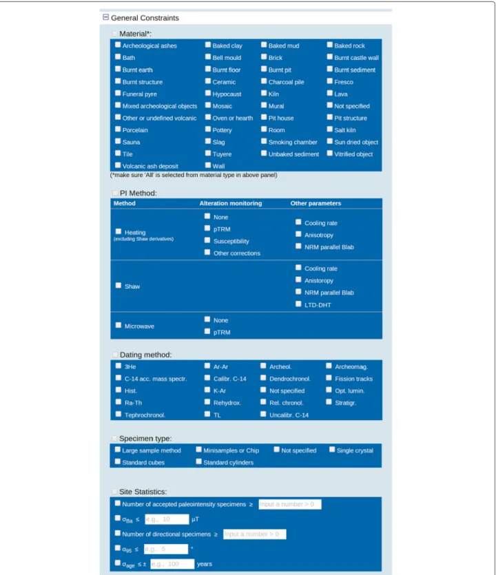
Methods based upon different underlying principles to the Thellier-type methods are also included: (1) the Shaw (1974) technique and variants of, e.g., Evans (1986); Rolph and Shaw (1985); Tsunakawa and Shaw (1994); Yamamoto et al. (2003); (2) the multispecimen parallel differential pTRM method (Dekkers and Böhnel 2006) and variants (Fabian and Leonhardt 2010); (3) the con-tinuous high-temperature triaxe method (Le Goff and Gallet 2004) based upon the method of Boyd (1986); and (4) the method of Tanguy (1975), which incorpo-rates alteration correction. The user can select whether to query for data obtained from Thellier-type and other heating methods (excluding Shaw derivatives), Shaw-type methods, and microwave methods (‘General constraints’ section). Data from other methods, such as the Wilson method (Muxworthy 2010; Wilson 1961), the van Zijl method (van Zijl et al. 1962), and the Preisach method (Muxworthy and Heslop 2011) are currently not included in the database, but can be accommodated in future revisions.
Obtaining paleointensity from archeological and vol-canic materials is beset with problems. During paleoin-tensity experiments, two issues have commonly been observed: (1) physicochemical alteration of a specimen on heating causing a change in its magnetic proper-ties and (2) the influence of grains that are not non-interacting uniaxial single domain (SD), e.g., MD grains, and therefore do not follow the behavior predicted by SD theory (Néel 1949). Additional steps have been incor-porated in the design of paleointensity experiments to monitor changes in magnetization resulting from these two problems.
Monitoring the influence of alteration depends on the method. In variants of the Thellier and Thellier (1959) method, either thermal or by microwave excitation, rep-etition of lower temperature in-field steps can be used to assess whether alteration has occurred. If the mag-netization acquired between the initial heating step and the repeated step is significantly different, the specimen is thought to have altered. These steps are commonly referred to as pTRM checks (see Tauxe and Yamazaki 2007 for a fuller explanation). It is noted in the database whether pTRM checks have been used and searches can be refined to select intensity data obtained only from experiments incorporating pTRM checks (‘General con-straints’ section). However, when treated alone, posi-tive pTRM checks do not guarantee the accuracy of the paleointensity data. At least three caveats to the effec-tiveness of pTRM checks have been noted. Firstly, fail-ure of pTRM checks can result from MD grains (Biggin 2010) (checks for MD behavior are described later in this section). Secondly, pTRM checks may pass (and the rela-tionship between NRM and pTRM remain linear) when alteration produces grains with blocking temperatures higher than can be assessed by the check. The NRM may be remagnetized, but alteration will not necessarily be visible in the pTRM checks (see Valet (2003)). In this instance, the demagnetization components of the NRM will not tend to zero, but will tend towards the labo-ratory field. Thirdly, inaccuracies can result from mea-surement noise in low NRM intensity specimens (Bowles et al. 2006) and additional experimental uncertainties (Paterson et al. 2012).
It has been proposed that the difference between the pTRM check and the initial pTRM can be used to correct for alteration (Valet et al. 1996) and some entries in the database have data corrected in this manner (e.g., Valet et al. (1998)). The alteration correction method of Walton (1990) applicable to Thellier-type measurements is noted in the database, although can not be searched for. Cau-tion must be taken when correcting pTRM for changes in magnetization resulting from alteration (Perrin et al. 1998).
In some studies measurements of susceptibility before and after acquisition of each pTRM have been used to monitor alteration (e.g., Coe (1967a); Gonzalez et al. (1997)) or a propensity to alter has been inferred from differences in susceptibility on heating and cooling in temperature-susceptibility curves, with some studies using this as a pre-selection method (e.g., Hartmann et al. (2011)). Alteration assessed using susceptibility is noted in the database and paleointensity data be can chosen by whether susceptibility was used as an alteration moni-tor (‘General constraints’ section). However, it has long been noted that changes in susceptibility may not mimic alteration of the remanence carriers (Coe 1967a; Thellier
and Thellier 1959). Remanence carriers may only com-prise a small fraction of the total magnetic contribution and the proclivity of each fraction to alter may differ. This may result in specimens acceptable for paleointen-sity being excluded based upon changes in susceptibility (Coe 1967a) or specimens showing limited susceptibility change being unsuitable for paleointensity analysis (e.g., Kosterov and Prévot (1998)).
Other alteration monitors or corrections used in Thel-lier double-heating methods are not explicitly stated in the database (e.g., Burakov and Nachasova (1985)), but are classed as ‘Other correction’. They can be used to refine the data search purely on the existence of some non-specific form of check or correction (‘General constraints’ section).
Changes in anhysteretic remanent magnetization (ARM) may mimic changes in TRM and have been used to monitor alteration. In the Shaw (1974) method, AF demagnetized ARMs acquired before and after the appli-cation of the total TRM step are used to assess alteration. Furthermore, expanding upon the idea of Kono (1978), Rolph and Shaw (1985) used the ratio of the pre- and post-heating ARMs to correct for non-linear alteration of the TRM at the same AF steps. The Rolph and Shaw (1985) correction to Shaw (1974) data is noted in the database. However, the degree to which ARM can correct for alteration of TRM is unclear (Tanaka and Komuro 2000; Valet and Herrero-Bervera 2009). To test the appli-cability of the ARM correction, Tsunakawa and Shaw (1994) incorporated a second TRM step: the double heat-ing test (DHT). This compares the first TRM with the second TRM corrected using the ratio of ARMs before and after the second heating. If the difference between the two TRMs is greater than the experimental error, it is assumed that the ARM correction does not fully cor-rect or over corcor-rects the paleointensity estimate. As with methods to correct for alteration during Thellier-type methods, this correction should be treated with caution, especially for cases when the ratio of the pre- and post-heating ARMs is far from unity; however, this correction is a standard step in more recent applications of the Shaw (1974) method (e.g., Yamamoto et al. (2003)).
The presence of MD grains has long been known to cause a non-linearity between NRM lost and pTRM gained in Thellier-type experiments (Levi 1977). This results in a concave curvature on a standard Arai-Nagata plot (Nagata et al. 1963). This curvature is typically assessed visually; however, the degree of curvature can be quantified (e.g., Paterson 2011), allowing MD domi-nated specimens to be isolated and removed from further analysis. Whether curvature was observed is currently not noted in the database, but would be a useful addition in any future revision. However, substantial non-linearity may not always be appreciable on an Arai-Nagata plot, yet
paleointensity results may be biased by the presence of MD grains (Riisager and Riisager 2001), as MD grains can result in additional effects that may influence the outcome of paleointensity experiments (see Dunlop (2011) and ref-erences therein). Unlike for SD grains, pTRMs held by MD grains are not independent. This can result in undemag-netized pTRM after zero-field heating, referred to as a high temperature thermal demagnetization tail. Building upon earlier work, Riisager and Riisager (2001) suggested the presence of high temperature thermal demagnetiza-tion tails could be monitored in the Coe-Thellier method by applying zero-field steps at the same temperatures as preceding in-field steps. If the zero-field step did not result in full demagnetization of the pTRM, then a ther-mal demagnetization tail remained (i.e. a difference in the NRM of the zero-field steps either side of the in-field step) and the paleointensity estimate could be rejected. They termed this a ‘pTRM-tail check’. We note whether a tail check was performed, but it is not currently pos-sible to restrict the database output for paleointensity experiments that incorporated this check. Additionally, one must be mindful that tail checks can be calculated in a number of ways (e.g., Leonhardt et al. (2004b); Yu and Dunlop (2003)) and different limits may have been placed on the statistical acceptability of the checks depending upon the study.
An alternative approach is to reduce the influence of MD grains. Low-temperature demagnetization (LTD) can be an effective method of removing MD remanence held by magnetite (e.g., Ozima et al. (1964); Yu et al. (2003)). Although rarely employed within Thellier-like experi-ments, as it is required after each heating step and the experiment is already lengthy, LTD is commonly used as a modification to the Shaw (1974) method (e.g., Yamamoto et al. (2003)). It is noted in the database whether this method was employed. Paleointensity data retrieved by the database can be limited to those obtained using the Shaw (1974) method with additional LTD and DHT steps (‘General constraints’ section).
For archeological materials, two further corrections are frequently applied: (1) for the difference between cool-ing rates in the laboratory and at the time of fircool-ing, e.g., for kilns; and (2) for remanence anisotropy. The TRM acquired by a material is related to the time it takes to cool coupled with its magnetic grain size distribu-tion (see Biggin et al. 2013 and Ferk et al. 2014 and references therein for a history of the subject). If for non-interacting SD grains the difference between the natural cooling and laboratory cooling is different, then the fun-damental equation relating the ratio of these two TRMs to the ratio of the ancient to laboratory field is violated and a correction to the paleointensity estimate should be attempted. Many fired archeological materials con-tain non-interacting SD particle assemblages and a strong
cooling rate dependence has been demonstrated (e.g., Fox and Aitken (1980)). Two approaches can be used to cor-rect for cooling rate: theoretically or experimentally. If the time taken to cool naturally is known or estimated and the grain size is assumed to be SD, then non-interacting SD theory can be applied to calculate the difference in TRM acquired on cooling in the laboratory and after firing (e.g., Halgedahl et al. (1980)). As fired archeological mate-rials are often thermally stable (resulting from acquiring their remanence originally from reheating), then it is pos-sible to experimentally determine the cooling rate effect without the complication of altering the TRM (e.g., Gen-evey and Gallet (2002)). We note in the database whether either of these approaches have been applied and it is pos-sible to restrict the database output to only paleointensity results corrected for cooling rate dependence (‘General constraints’ section).
For grains other than non-interacting SD, the effect could be much smaller or even negligible, e.g., for MD grains, and a correction may not be necessary (Biggin et al. 2013; Ferk et al. 2014). This may be the case for many vol-canic rocks. In addition, although cooling of lavas can take (with the exception of the margins) a few days to months, cooling rate corrections have rarely been attempted. To assess cooling rate dependence, the specimen must be heated above the Curie temperature, and in volcanics, this often results in alteration. It is therefore not possible to obtain reliable measurements of the cooling rate effect on the TRM (unless, in some cases, performed in a controlled atmosphere). For finer grained rocks, e.g., volcanic glass, cooling rate can be an issue (Ferk et al. 2010; Leonhardt et al. 2006); however, it is dependent on the difference between the laboratory and natural cooling rates (Bowles et al. 2005).
Archeological materials manipulated by hand or machine can preferentially align magnetic grains within the material. This is common, e.g., in pottery, where clay is stretched and molded. This can result in anisotropy of the TRM, with an easy direction of magnetization within the shear plane of the material (e.g., Rogers et al. (1979)). This can significantly bias paleointensity estimates as the TRM acquired is dependent on the angle between the remanence direction and the laboratory field. Different experimental approaches can be taken to address rema-nence anisotropy. To minimize the angular difference, the specimen can be aligned so its NRM is parallel with the laboratory field during the paleointensity experiment (e.g., Fox and Aitken (1980); Rogers et al. (1979)). This can be technically difficult. Alternatively, remanence anisotropy can be described by a second rank tensor and the paleointensity corrected (Veitch et al. 1984). A series of TRM, ARM, isothermal remanance (IRM), or suscep-tibility measurements can be made after or at some point during a paleointensity experiment (Chauvin et al. 2000)
to define the TRM ellipsoid; however, caution should be used when using an induced remanence other than a TRM (Chauvin et al. 2000). An anisotropy correction can be applied to paleointensity data obtained from any method. The type of anisotropy correction is noted in the database and listed at http://geomagia.gfz-potsdam. de/ID_glossary.php#PIANID. Whether an anisotropy correction has been used is a selection criterion limiting the output of the database for all methods except the microwave method (‘General constraints’ section).
The number samples (NBa) used in the calculation of a
mean paleointensity, the number of specimens measured for paleointensity analysis (nBameas.), and the number of
specimens accepted (nBa acc.) for the calculation of the
mean paleointensity are noted in the database. The mini-mum number of specimens required to produce a reliable estimate has been discussed (e.g., Biggin et al. (2003); Paterson et al. (2010)), see also Suttie et al. (2011). These metadata may aid future analyses in this topic. As noted in the ‘Paleomagnetic data’ section, the type of uncer-tainty reported on the mean is not currently listed in the database; however, if the user wishes to calculate, for example, the standard error of the mean as a measure of uncertainty rather than the standard deviation, the num-ber of accepted specimens is required. The numnum-ber of accepted specimens (or accepted samples, if the number of accepted specimens is not given) can be used to restrict the output of the paleointensity data (‘General constraints’ section); however, it is recommended to proceed with caution when selecting a cut-off.
Chronological metadata
Dating methods for archeomagnetic materials vary. They include historical documentation, archeological evidence such as typologically defined epochs, stratigraphic infor-mation, and a range of physical/chemical/environmental methods, for instance radiocarbon dating (for a review, see Aitken (1999)). Volcanic materials are primarily dated by isotopic methods, e.g., by K-Ar, 40Ar/39Ar, and radiocarbon dating (see the ‘Chronological data’ section); however, more recent volcanic materials have been dated through historical observations. In total, 18 dating methods are accommodated in the database. They are listed at http://geomagia.gfz-potsdam.de/ID_glossary. php#DatMethod.
Knowing the type of dating method can aid in assess-ing the reliability of an age, and the database allows the user to select data based upon specific dating types (see the ‘General constraints’ section). Unfortunately, approx-imately 30% of ages are from unspecified methods. Along with ages based upon archeological evidence (approxi-mately 40%), radiocarbon ages (approxi(approxi-mately 15%), and historical ages (approximately 10%), these four cate-gories account for approximately 95% of all age data.