Transient residence and exposure times

(1)

HAL Id: hal-00298433

https://hal.archives-ouvertes.fr/hal-00298433

Submitted on 26 May 2005

HAL is a multi-disciplinary open access

archive for the deposit and dissemination of sci-entific research documents, whether they are pub-lished or not. The documents may come from teaching and research institutions in France or abroad, or from public or private research centers.

L’archive ouverte pluridisciplinaire HAL, est destinée au dépôt et à la diffusion de documents scientifiques de niveau recherche, publiés ou non, émanant des établissements d’enseignement et de recherche français ou étrangers, des laboratoires publics ou privés.

Transient residence and exposure times

E. J. M. Delhez

To cite this version:

E. J. M. Delhez. Transient residence and exposure times. Ocean Science Discussions, European Geosciences Union, 2005, 2 (3), pp.247-265. �hal-00298433�

(2)

OSD

2, 247–265, 2005

Transient residence and exposure times

E. J. M. Delhez Title Page Abstract Introduction Conclusions References Tables Figures J I J I Back Close

Full Screen / Esc

Print Version Interactive Discussion

EGU

Ocean Science Discussions, 2, 247–265, 2005 www.ocean-science.net/osd/2/247/

SRef-ID: 1812-0822/osd/2005-2-247 European Geosciences Union

Ocean Science Discussions

Papers published in Ocean Science Discussions are under open-access review for the journal Ocean Science

Transient residence and exposure times

E. J. M. Delhez

University of Li `ege, Belgium

Received: 11 April 2005 – Accepted: 13 May 2005 – Published: 26 May 2005 Correspondence to: E. J. M. Delhez (e.delhez@ulg.ac.be)

(3)

OSD

2, 247–265, 2005

Full Screen / Esc

EGU

Abstract

The residence time measures the time spent by a water parcel or a pollutant in a given water body and is therefore widely used in environmental studies. The adjoint method introduced by Delhez et al. (Estuarine Coastal and Shelf Sciences, 2004) to compute this diagnostic is revised here to take into account the effect of the initialisation and of 5

the boundary conditions.

In addition to the equation for the mean residence time, it is suggested to solve a simple advection-diffusion problem to quantify the effect of the initialisation and clarify the interpretation of the results.

Using the two same equations but with modified boundary conditions, the method 10

can also be used to quantify the accumulated time spent by water/tracer parcels in a control domain. This diagnostic is called “exposure time”.

1. Introduction

The residence time of a water parcel in a water body is usually defined as the taken by this parcel to leave this water body (e.g. Bolin and Rhode,1973;Takeoka,1984; 15

Zimmerman,1988;Monsen et al.,2003;Braunschweig et al.,2003). As such, it is a valuable diagnostic tool to describe and understand environmental issues.

Basically, the residence time is a property of each water parcel; it is Lagrangian by nature. Indeed, the straightforward procedure to asses the residence time consists in injecting some tracer in the flow, following the path of these tracers parcels and 20

registering the time when they leave the domain of interest. This procedure can be equally applied in real world experiments or in numerical model simulations.

Mathematically, the mean residence time ¯θ(t, x) at time t and location x can be

com-puted by monitoring the temporal evolution ˜m_(t,x)(t+τ) of the mass of the tracer at the time t+τ after a unit point release at (t, x). Following Bolin and Rhode (1973) and 25

(4)

OSD

2, 247–265, 2005

Full Screen / Esc

EGU

Takeoka(1984), one can write

¯

θ(t, x)=

Z1 0

τ dm˜_(t,x) (1)

Delhez et al.(2004) introduced an alternative procedure designed for numerical mod-els. They showed that the residence time can be computed as the solution of an advection-diffusion problem with a unit source term and appropriate boundary condi-5

tions. The method provides the variations in space and time of the residence time with a single model run. The method doesn’t require any Lagrangian module. It is Eulerian by nature which makes it more appropriate to long-term and large scale simulations than the straightforward Lagrangian approach. Considering the potential discrepancies between the Lagrangian and Eulerian descriptions of diffusion, the Eulerian approach 10

of the residence time is closer to the Eulerian hydrodynamic models and represents a more direct diagnostic of the model results.

In their paper, Delhez et al. (2004) raised the issue of the appropriate definition of the residence time when water parcels leaving the domain of interest are allowed to re-enter at later times. They also mention the problem associated with the fact that a 15

finite range simulation cannot provide the residence time of all the water parcels nor the mean residence time.

The purpose of this paper is to clarify these two issues and complement the adjoint method advocated byDelhez et al. (2004) with appropriate definitions and additional control variables.

20

2. Backward procedure for the computation of the residence time

Because of diffusion, different water parcels released at the same location and the same time follow different paths, exit the control domain ω at different times and have therefore different residence times in ω. To describe this situation,Delhez et al.(2004) define the cumulative distribution function D(t, τ, x) as the fraction of the mass of the 25

(5)

OSD

2, 247–265, 2005

Full Screen / Esc

EGU

tracer released at time t and location x whose residence time is larger or equal to τ. This is also the mass of tracer in the control region at time t+τ following a unit release at time t and location x, therefore

D(t, τ, x)= ˜m_(t,x)(t+ τ) (2)

This cumulative distribution function is shown to satisfy 5    ∂D ∂t − ∂D ∂τ + v · ∇D + ∇ · h K · ∇Di = 0 D(t, 0, x)= δ_ω(x) (3)

where v is the velocity vector, K denotes the symmetric diffusion tensor and

δ_ω(x)=

(

1 if x ∈ ω

0 if x 6∈ ω (4)

is the characteristic function of the control region ω.

The zeroth order moment of the cumulative distribution function, i.e. 10 ¯ θ(t, x)= Z∞ 0 D(t, τ, x)d τ (5)

is the mean residence time if D satisfies particular boundary conditions (Delhez et al.,

2004).

Assuming that D(t, τ, x) decreases to zero when τ tends to infinity, i.e. that the whole material is eventually flushed out of the control region, Eq. (3) can be integrated with 15

respect to τ to simplify the problem into the more classical differential problem

∂ ¯θ

∂t + δω+ v · ∇ ¯θ + ∇ ·

h

K· ∇ ¯θi = 0 (6)

for ¯θ(t, x). For ¯θ to be equal to the mean residence time, Eq. (6) must be solved with the boundary condition that ¯θ vanishes on the boundary δω of the control domain.

(6)

OSD

2, 247–265, 2005

Full Screen / Esc

EGU

Equations (3) and (6) are derived from the adjoint of the forward advection-diffusion problem. They must therefore be integrated backwards in time with homogeneous boundary conditions. The integration backwards in time is clearly necessary for stability reasons associated with the apparent negative diffusion term in Eqs. (3) and (6). It is also a consequence of the fact that one does not know in advance the fate of the 5

particles.

3. Finite range simulation

In principle, Eqs. (3) and (6) must be integrated backwards from t=+∞ in order to be able to describe the full distribution of residence times, including the fate of particles with a very large residence time. In practice, of course, the equation is integrated 10

backwards from some finite time T at which the real conditions are unknown. As a result, the solution will not provide the exact mean residence time until the uncertainty about the initial conditions has disappeared. Intuitively, one can expect that the effect of the initial conditions smears out after a period of integration of several multiples of the residence time.

15

A more accurate appraisal of the effect of the initial conditions can be given by a careful analysis of Eq. (3). Clearly, the uncertainty about what happens after the “initial” time T affects only the cumulative distribution D(t, τ, x) in the range of τ>T −t. As t decreases, while proceeding with the backward integration, an increasing portion of the distribution of the residence time is uncovered.

20

If the initial condition at time T is D=0, then D is also zero for all τ>T −t, Z∞ 0 D(t, τ, x)d τ= ZT−t 0 D(t, τ, x)d τ (7)

and the solution ¯θ of Eq. (6) characterises only the water parcels with a residence time smaller than T − t. While ¯θ tends to the mean residence time for large values of T − t,

the actual rate of convergence is not known. 25

(7)

OSD

2, 247–265, 2005

Full Screen / Esc

EGU

To quantify the proportion of water parcels whose contribution is taken into account

in ¯θ, we propose to solve the adjoint problem

     ∂C_T∗ ∂t + v · ∇C ∗ T + ∇ · h K · ∇C∗_Ti = 0 C∗_T(T , x)= δ_ω(x) (8)

in addition to Eq. (6). After Delhez et al. (2004), the solution C_T∗(t, x) of this problem can indeed be interpreted as the proportion of the initial point release at (t, x) that is 5

still present in the control domain at time T . Conversely, ˜

C_T∗(t, x) ≡ 1 − C_T∗(t, x) (9)

represents the proportion of water parcels whose residence time can be computed with a model run in the time window [t, T ]. This quantity can be used to quantify the representativeness of the solution of Eq. (6) as the mean residence time.

10

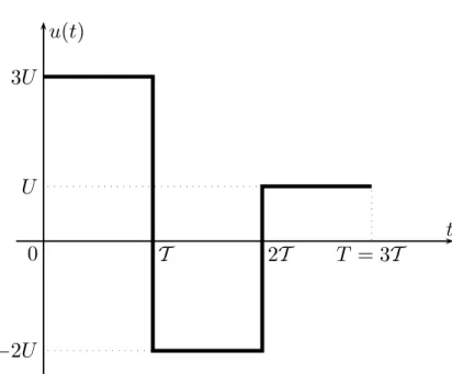
To clarify the concepts introduced in this section, it is interesting to consider the highly idealised system of a one-dimensional domain x ∈]−∞, ∞[ and compute the mean residence time in the control domain ω=]−∞, 0]. We assume that the velocity field is uniform but varies with time as in Fig.1. Diffusion is first neglected to ease the understanding.

15

From the discussion above, the mean residence time is obtained as the solution ¯θ of

   ∂ ¯θ ∂t + u(t) ∂ ¯θ ∂x + 1 = 0, x∈ ω ¯ θ(t, 0)= 0 when u(t) > 0 (10)

This equation must be integrated backwards from some “initial” time T . As the true “initial” conditions at that time are unknown we take

¯

θ(T , x)= 0 (11)

(8)

OSD

2, 247–265, 2005

Full Screen / Esc

EGU

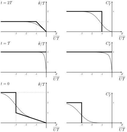
The solution of the problem (Eqs.10–11) at different times is shown in Fig.2. At time t=2T , the residence time varies linearly between T at x=−UT and 0 at x=0. This is precisely the time for a water parcel to be advected from its location at t=2T to the boundary of the control domain by the velocity field U acting between t=2T and

t=3T .

5

The residence time for x<−U T seems to be a constant, equal to the elapsed time T of the backward simulation. This is however an artefact of the initialisation of the computation at time T . The water parcels released at x<−U T at time t=2T do not have time enough to exit the control domain; they are still in ω at t=T . Therefore the residence time of these water parcels cannot be settled since their exit time is unknown. 10

The resolution of the appropriate form of Eq. (8),            ∂C_T? ∂t + u(t) ∂C_T? ∂x = 0, x ∈ ω C?_T(T , x)= 1, x ∈ ω C?_T(t, 0)= 0 when u(t) > 0 (12)

is useful to identify the part of the solution of Eq. (10) that is affected by the initialisation and/or cannot be interpreted as the residence time. The solution C?_T plotted in Fig.2

confirms that the particles located at x<−U T at time t=2T do not leave the domain 15

during the simulation period.

A quick look at the distribution of C_T? at t=T , tells us that none of the particles present in the control domain at this time can leave the control domain before t=T . Their residence time is therefore unknown. The value of ¯θ is just a lower bound of the

residence time. 20

A similar analysis can be done from the results at t=0. In this case, the residence time increases linearly from zero at the origin to T at x=−3UT . The residence time cannot be computed in the leftmost part of the control domain.

(9)

OSD

2, 247–265, 2005

Full Screen / Esc

EGU

this case, one must solve            ∂ ¯θ ∂t + u(t) ∂ ¯θ ∂x + κ ∂2θ¯ ∂x2 = 0, x∈ ω ¯ θ(T , x)= 0, x ∈ ω ¯ θ(t, 0)= 0 (13) and            ∂C_T? ∂t + u(t) ∂C_T? ∂x + κ ∂2C¯_T? ∂x2 = 0, x∈ ω C?_T(T , x)= 1, x ∈ ω C?_T(t, 0)= 0 (14)

by backward integration from t=T . Similar conclusions are obtained with, of course, 5

smoother spatial distributions of the residence time and of C_T?. Because of diffusion, the initialisation is seen to affect the results in a larger part of the control domain and/or for earlier times t. The spatial distribution of C_T? is not strictly equal to unity in the control domain, even in its leftmost part. This shows that some water parcel can now escape the control domain by diffusion within the studied time window. In such areas, 10

¯

θ provides a lower bound for the residence time but cannot be interpreted as a valid

approximation of the residence time unless C_T?is close to zero.

The computation of C_T∗ is useful to check the influence of the initialisation a posteriori,

i.e. once the simulation has been carried out. For practical applications, it is also desirable to have some a priori estimates of the spin-up time. A compromise must 15

indeed be found between the necessity to take the “initial time” T as large as possible to remove the effect of the initialization and the wish to reduce the length of the numerical simulations. Obviously, the ideal duration of the simulation depends on the residence time it-self; the larger the residence time, the larger the duration of the simulation. As a rule of thumb, one could argue that the simulation window [t, T ] should be as large 20

(10)

OSD

2, 247–265, 2005

Full Screen / Esc

EGU

as twice the mean residence time for the results at time t to be significant. As the residence time is not known a priori, rough estimates based on simplified models can be used to chose T .

In an advection dominated flow, the backward integration of Eq. (8) produces a front generated at the boundary of the control domain and moving into it. If Uc denotes 5

the characteristic velocity of the flow and if the model is allowed to spin-up for ∆t, then the space swept by the front during that time interval can be characterized by the advective length scale Uc∆t. In the meantime, horizontal diffusion smears out the front over a length scale which is some multiple α, say α=3, of the diffusion length scale√Kc_{∆t where K}c_{is some characteristic (explicit and implicit) horizontal di}_ffusion

10

coefficient. This spreading reduces the influence of the boundary signal in the interior of the control domain. Therefore, C_T∗ will be close to zero only at locations whose distance to the outflow boundary of the control domain is less than

Lc_{= U}c_{∆t − 3}p_Kc_∆t ₍₁₅₎

At such locations, the residence time can be reasonably obtained from the solution of 15

Eq. (6) after a spin-up time of∆t. If L denotes the horizontal dimension of the whole control domain, then the model should be allowed to spin-up for∆t such that

L≤ Lc_{= U}c_{∆t − 3}p_Kc_∆t ₍₁₆₎

The estimate Eq. (15) applies reasonably well to the 1D case discussed above if the reversal of the flow (Fig.1) is properly taken into account. For instance, considering the 20

initialisation at t=T and looking at the results at t=2T , Eq. (15) gives (taking Uc=3U and Kc=U2T /4)

Lc_{= −1.5UT} ₍₁₇₎

which confirms that the residence time computed by Eq. (6) cannot be considered to be significant at any point of the control domain (Fig.2). For the conditions prevailing 25

(11)

OSD

2, 247–265, 2005

Full Screen / Esc

EGU

for t ∈ [0, T ] (Uc=3U and Kc=U2T /4) Eq. (15) predicts that the initialisation at time

t= T would produce reasonable estimates of the residence time at t=0 for

x > 1.5U T (18)

which can be confirmed by inspection of Fig.2.

4. Residence time and exposure time

5

The physical interpretation of ¯θ as the mean residence time in the control domain ω

depends on the boundary conditions used to solve Eqs. (3) or (6).

The residence time is usually defined as the time taken for a water parcel to leave the control domain for the first time (e.g.Bolin and Rhode,1973;Takeoka,1984;

Zimmer-man, 1988;Monsen et al.,2003). To compute this diagnostic, called strict residence 10

time inDelhez et al.(2004), Eq. (3) or Eq. (6) must be solved with homogenous bound-ary conditions prescribed on the boundbound-ary δω of the control domain ω. In particular, ¯θ

must vanish at the boundary of the control domain.

With such boundary conditions, water parcels leaving the domain at some time are not allowed to re-enter and D(t, τ, x), which represents the mass in the control domain 15

at time t+τ after a unit injection, is a decreasing function of τ. This decreasing behavior is of course expected from the interpretation of D as a cumulative distribution function. It is also required to transform the usual definition of the residence time Eq. (1) into

(12)

OSD

2, 247–265, 2005

Full Screen / Esc

Print Version Interactive Discussion EGU Eq. (5) along ¯ θ(t, x)= Z1 0 τ dm˜_(t,x) = − Z∞ 0 τ d ˜ m_(t,x) d t (t+ τ)dτ = −hτm˜_(t,x)(t+ τ)i∞ 0 + Z∞ 0 τm˜_(t,x)(t+ τ)dτ =Z∞ 0 ˜ m_(t,x)(t+ τ)dτ =Z∞ 0 D(t, τ, x)d τ= ¯Θ(t, x) (19) 5

(assuming that ˜m_(t,x)decreases to zero for large τ).

In Delhez et al. (2004), it is proposed to solve Eq. (3) or Eq. (6) with boundary conditions allowing the water parcels to re-enter in the control domain. In this case, the mass ˜m_(t,x)(t+τ) is no longer a decreasing function of the delay τ. Therefore, the first equality in Eq. (19) is not valid and the solution of Eqs. (3) or (6) cannot be interpreted 10

as the residence time any more. Still D and ¯θ have an interesting interpretation: they

can be regarded as measures of the total time spent by the water parcels in the control domain. In particular, ¯θ measures the area under the curve ˜m_(t,x)(t+τ) for the whole range of values of τ (or τ in [0, T −t] for finite range simulations). We propose therefore to call this quantity ‘exposure time’.

15

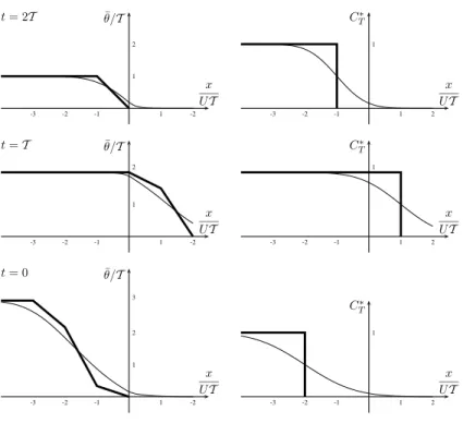
The concept of exposure time and its computation can also be demonstrated with the idealized one-dimensional system introduced above. This time, Eq. (6) and Eq. (8) must be solved in the whole spatial domain x ∈]−∞, ∞[ without prescribing auxiliary conditions at the boundary x=0 of the control domain. The results are shown in Fig.3. At all times and locations, the value reported for ¯θ measures the total time spent by

20

the water parcels in the control domain between the current time t and the initialisation time T . The value of C∗_T can be used to identify the water parcels that are still in the control domain at t=T and those which left (and did not re-enter) the domain before that time.

(13)

OSD

2, 247–265, 2005

Full Screen / Esc

EGU

At t=2T , the spatial distributions of ¯θ and C∗_T are identical to those computed in the previous section. This is of course due to the fact that the velocity is positive for

t∈]2T , 3T [, i.e. that all the water parcels are leaving the control domain.

Between t=2T and t=T , all the water parcels that left the domain are advected back into the control domain by the reversing flow (Fig.1). The value of ¯θ plotted in the left

5

panel for t=T is affected by the initialisation at t=T in the range x<UT as shown by the value of C_T? in this part of the domain. The results for x>U T are not affected by the initialisation. The values reported for ¯θ in this range can therefore be understood

as the true exposure time of the water parcels, i.e. as a measure of the time spent by the water parcels in the control domain. This measure is representative inasmuch as 10

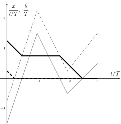
the water parcels have left the control domain before t=T . Of course, a reversal of the flow at t>T could however push the parcels back into the control domain at later times. Particles in x<−2U T at t=0 are still in the control domain at t=T while those located at x>−2U T at time t=0 have all left the control domain at t=T . The latter exhibit exposure times between 0 and 2T . The stair-case distribution of ¯θ reflects the different

15

paths of the parcels. As shown in Fig.4 in the particular case of particles released at

x=−1.5UT and x=−0.75UT , some particles are present in the control domain during

two distinct time intervals while others spent their time in ω in one single time interval. In both cases, the exposure time is the accumulated time spent in the control domain.

Similar results are obtained when diffusion is added to the system (Fig.3). As for the 20

residence time, the spatial distribution are smoother and the effect of the initialisation is increased by diffusion. This last effect appears even worse in Fig.3 than in Fig.2. There is indeed no strong boundary condition at x=0 which can constrain the solution and make it converge faster.

5. Final comments

25

The method introduced by Delhez et al.(2004) for the numerical computation of the residence time is a powerful and versatile tool. It can also be used, with appropriate

(14)

OSD

2, 247–265, 2005

Full Screen / Esc

EGU

boundary conditions, to quantify the total time spent by water or tracer parcels in a control domain through what we call the ‘exposure time’.

To assess the influence of the initialisation and support the physical interpretation of the results, it is proposed to solve Eq. (8) in addition to Eq. (6).

The two Eqs. (8) and (6) are very similar to the two equation system introduced by 5

Delhez et al.(1999) to compute the age of tracers. In the case of a conservative tracer, these can be written as

∂C ∂t + v · ∇C = ∇ · (K · ∇C) (20) and ∂α ∂t + v · ∇α = C + ∇ · (K · ∇α) (21) 10

where C is the concentration of the tracer and α is the so-called age concentration. The mean age ¯a is related to C and α by

¯

a= α

C (22)

The method discussed here for the computation of the residence time can therefore be understood as an extension of the Constituent-oriented Age Theory (Delhez et al., 15

1999;Deleersnijder et al., 2001;Delhez and Deleersnijder,2002). This consolidated theory is hence called “Constituent-oriented Age and Residence time Theory” (CART). In the system (Eqs. 20–21), C measures the concentration of the tracer that, tak-ing into account the effect of initialisation, contributes to the age concentration. It plays therefore a similar part as C∗_T in the computation of the residence time. The 20

age concentration α accumulates the contributions to the mean age of the different tracer parcels forming C. It is comparable to ¯θ.

From this similarity of the concepts, it is tempting to modify the definition of the mean residence time according to

¯

θ

C∗_T (23)

(15)

OSD

2, 247–265, 2005

Full Screen / Esc

EGU

as only the water parcels forming C∗_T are taken into account in ¯θ. This ratio would

be interpreted as the mean residence time of the water parcels in C_T∗. However, this approach is not appropriate. The residence time is a Lagrangian property inasmuch as it can be computed for each and every water parcel by attaching a ‘virtual clock’ to each parcel and recording its exit time from the control domain. But the path of a single 5

virtual water parcel subjected to Fickian diffusion does not make sense in its own. The paths of different parcels forming a given patch are not independent from each other. This is best demonstrated by the contradiction which arises if one selects the parcels accounting for ˜C_T∗(t₀, x)=1−C∗_T(t₀, x) at some initial time t₀<T and use this as initial

conditions of a forward simulation; while the definition of ˜C∗_T implies that it vanishes in 10

the control domain at time T , the forward simulation will produce a non zero distribution at that time. The particles accounting for ˜C_T∗(t₀, x) all manage to escape the control

do-main only because other particles immersed in the same diffusive environment remain in ω. With the Fickian model of diffusion, it is impossible to separate the fate of the particles that leave the control domain within a given time window and those that do 15

not. The arguments leading to Eq. (23) are therefore inappropriate.

References

Bolin, B. and Rhode, H.: A note on the concepts of age distribution and residence time in natural reservoirs, Tellus, 25, 58–62, 1973. 248,256

Braunschweig, F., Martins, F., Chambel, P., and Neves, R.: A methodology to estimate renewal 20

time scales in estuaries: the Tagus Estuary case, Ocean Dynamics, 53, 3, 137–145, 2003.

248

Deleersnijder, E., Campin, J.-M., and Delhez, E. J. M.: The concept of age in marine modelling: I. Theory and preliminary model results, Journal of Marine Systems, 28, 229–267, 2001. 259

Delhez, E. J. M., Campin, J.-M., Hirst, A. C., and Deleersnijder, E.: Toward a general theory of 25

the age in ocean modelling, Ocean Modelling, 1, 17–27, 1999. 259

(16)

Concen-OSD

2, 247–265, 2005

Full Screen / Esc

EGU

tration distribution function in the English Channel and the North Sea, Journal of Marine Systems, 31, 279–297, 2002. 259

Delhez, E. J. M., Heemink, A. W., and Deleersnijder, E.: Residence time is a semi-enclosed domain from the solution of an adjoint problem, Estuarine, Coastal and Shelf Science, 61, 691–702, 2004. 249,250,252,256,257,258

Monsen, N. E., Cloern, J. E., and Lucas, L. V.: A comment on the use of flushing time, residence 5

time and age as transport time scales, Limnology and Oceanography, 47, 5, 1545–1553, 2003. 248,256

Takeoka, H.: Fundamental concepts of exchange and transport time scales in a coastal sea, Continental Shelf Research, 3, 311–326, 1984. 248,249,256

Zimmerman, J. T. F.: Estuarine residence times, in: Hydrodynamics of estuaries, edited by: 10

(17)

OSD

2, 247–265, 2005

Full Screen / Esc

Print Version Interactive Discussion EGU

T = 3T

2T

T

0 3U

−2U

U

u(t)

t

(18)

OSD

2, 247–265, 2005

Full Screen / Esc

Print Version Interactive Discussion EGU x UT ¯θ/T -3 -2 -1 2 1 t = 2T x UT C∗ T -3 -2 -1 1 x UT ¯θ/T -3 -2 -1 2 1 t = T x UT C∗ T -3 -2 -1 1 x UT ¯θ/T -3 -2 -1 3 2 1 t = 0 x UT C∗ T -3 -2 -1 1

Fig. 2. Temporal evolution of ¯θ and C_T∗ from a backward integration of the equations for the mean residence time from t=T . Results without diffusion (thick curve) and with diffusion (thin curve, κ=U2_{T /4).}

(19)

OSD

2, 247–265, 2005

Full Screen / Esc

Print Version Interactive Discussion EGU x UT ¯θ/T -3 -2 -1 1 -2 2 1 t = 2T x UT C∗ T -3 -2 -1 1 2 1 x UT ¯θ/T -3 -2 -1 1 -2 2 1 t = T x UT C∗ T -3 -2 -1 1 2 1 x UT ¯θ/T -3 -2 -1 1 -2 3 2 1 t = 0 x UT C∗ T -3 -2 -1 1 2 1

Fig. 3. Temporal evolution of ¯θ and C∗_T from a backward integration of the equations for ex-posure time from t=T . Results without diffusion (thick curve) and with diffusion (thin curve,

(20)

OSD

2, 247–265, 2005

Full Screen / Esc

Print Version Interactive Discussion EGU 3 2 1 −1 2 1

x

UT

,

¯θ

T

t/T

Fig. 4. Temporal evolution of the location (thin curve) and exposure time (thick curve) of