HAL Id: hal-01622252
https://hal.archives-ouvertes.fr/hal-01622252
Submitted on 24 Oct 2017
HAL is a multi-disciplinary open access
archive for the deposit and dissemination of
sci-entific research documents, whether they are
pub-lished or not. The documents may come from
teaching and research institutions in France or
abroad, or from public or private research centers.
L’archive ouverte pluridisciplinaire HAL, est
destinée au dépôt et à la diffusion de documents
scientifiques de niveau recherche, publiés ou non,
émanant des établissements d’enseignement et de
recherche français ou étrangers, des laboratoires
publics ou privés.
Uncertainty management in stratigraphic well
correlation and stratigraphic architectures: A
training-based method
Jonathan Edwards, Florent Lallier, Guillaume Caumon, Cédric Carpentier
To cite this version:
Jonathan Edwards, Florent Lallier, Guillaume Caumon, Cédric Carpentier. Uncertainty management
in stratigraphic well correlation and stratigraphic architectures: A training-based method. Computers
& Geosciences, Elsevier, 2017, 111, pp.11-17. �10.1016/j.cageo.2017.10.008�. �hal-01622252�
Uncertainty management in stratigraphic well correlation and
stratigraphic architectures :
A training-based method
Jonathan Edwardsa, Florent Lallierb, Guillaume Caumona, C´edric Carpentiera
aGeoRessources (UMR 7359), Universit´e de Lorraine - ENSG, Vandoeuvre-l`es-Nancy, F-54500 France bTotal E&P UK, Aberdeen
Abstract
We discuss the sampling and the volumetric impact of stratigraphic correlation uncer-tainties in basins and reservoirs. From an input set of wells, we evaluate the probability for two stratigraphic units to be associated using an analog stratigraphic model. In the presence of multiple wells, this method sequentially updates a stratigraphic column defining the stratigraphic layering for each possible set of realizations. The resulting correlations are then used to create stratigraphic grids in three dimensions. We apply this method on a set of synthetic wells sampling a forward stratigraphic model built with Dionisos. To perform cross-validation of the method, we introduce a distance comparing the relative geological time of two models for each geographic position, and we compare the models in terms of volumes. Results show the ability of the method to automatically generate stratigraphic correlation scenarios, and also highlight some challenges when sampling stratigraphic uncertainties from multiple wells.
doi:10.1016/j.cageo.2017.10.008 Introduction
The sedimentary record is generally accessible only at a small set of locations (wells or outcrops) or through geophysical images of limited spatial resolution. Stratigraphic correlation of such sparse data is essential to characterize the history and the proper-ties of sedimentary basins, to determine unit geometries and the volumes of sediment deposited through time, for example. It has, therefore, strong implications for under-standing the complex interactions between climate, erosion, sedimentation and tectonics
in siliciclastic environments (see for instance Molnar and England (1990); Burbank et al. (1996); M´etivier et al. (1999); Rouby et al. (2009); Charreau et al. (2011); Guillocheau et al. (2012); Bhattacharya et al. (2016); Herman and Champagnac (2016); Nicholson et al. (2016)). Stratigraphic correlations are also paramount to characterize stratigraphic architectures, their relation to facies distribution and their impact on fluid flow in the subsurface (Jackson et al., 2009; Lallier et al., 2012; Cavero et al., 2016).
As with all interpretative processes, stratigraphic correlation calls for ancillary knowl-edge to compensate for the lack or incompleteness of spatial observations. This concep-tual knowledge is very useful to obtain consistent interpretations, but it may also, if inappropriate, be a source of errors in the correlations and in further analysis. In the forward sense, it has also been shown that several depositional scenarios can produce the same succession of stratigraphic units (Helland-Hansen and Gjelberg, 1994; Armitage et al., 2015; Burgess and Prince, 2015), which motivates the consideration of multiple correlation hypotheses. Even under the same set of hypotheses, correlation lines can be uncertain and are not easily formulated in a systematic and repeatable way when drawn manually by experts (Borgomano et al., 2008; Koehrer et al., 2011; Colombera et al., 2012; Lallier et al., 2016).
Nonetheless, the range of possible stratigraphic correlations remains limited because spatial distribution of sediments are not random, but rely on sedimentological and phys-ical processes (Tetzlaff and Harbaugh, 1989; Lawrence et al., 1990; Kendall et al., 1991; Granjeon, 1997; Burgess, 2012; Wingate et al., 2016). These processes can be imple-mented in forward modeling software, which generate realistic 3D models to aid de-ciphering the relations between deposition parameters and stratigraphic architectures. Unfortunately, despite some successful attempts (Cross and Lessenger, 1999; Charvin et al., 2009; Falivene et al., 2014; Sacchi et al., 2015), conditioning forward stratigraphic models to seismic and well data remains a difficult computational challenge.
This paper builds on automatic stratigraphic well correlation methods, which make up an alternative option to generate consistent well correlations and to assess the asso-ciated uncertainties (Agterberg, 1990; Pels et al., 1996; Lallier et al., 2012; Agterberg et al., 2013; Lallier et al., 2016). Automatic correlation is reproducible, honors spa-tial observations and mitigates the subjectivity of interpretation. All existing automatic
correlation methods rely on elementary correlation costs that measure the dissimilarity between two observation points located on two distinct wells. In the case of regularly sampled well logs, the correlation coefficient within a depth window (Olea, 1994, 2004) or the Lp distance norm between log values (Gordon and Reyment, 1979; Wheeler, 2015) may be used for this purpose. As these costs do not fully reflect the reasoning made by expert-based correlation and do not easily account for sedimentary gaps, several authors propose to use a zonation of wells in terms of intervals and a specific distance function that reflects differences between interval features such as lithology and thickness (Smith and Waterman, 1980; Howell, 1983; Waterman and Raymond, 1987; Fang et al., 1992; Pels et al., 1996). Recently, Lallier et al. (2016) extended these rules for correlating car-bonate platform and ramp sediments using stratigraphic sequences and paleo-bathymetry interpreted along the wells. To gain more flexibility in the integration of sedimentological knowledge during correlation, a first contribution of this paper is to compute elementary correlation costs from analog numerical models (Section 2). To test this idea, we con-sider environments with uniform subsidence, and without active tectonics, which would perturb the sedimentation and create geometries more difficult to sample in an analog model.
Another aspect of automatic well correlation concerns the management of multiple wells. Indeed, as discussed by Lallier et al. (2016), the number of possible well corre-lations for several wells is extremely large in real situations. As a consequence, direct simultaneous correlation of multiple wells (Brown, 1997) is generally not feasible due to computational limitations. Wheeler (2015) address this problem by performing all possible pairwise correlations and then solving a global optimization problem to obtain a deterministic and consistent result. Alternatively, Lallier et al. (2016) propose to use a well traversal order and then to correlate pairs of wells sequentially along this path. Pairwise correlations may then be rebuilt to alleviate possible biases due to the traversal order. However, none of these methods can resolve layering ambiguities which may exist when gaps are present. This raises challenges for generating geometric realizations of 3D stratigraphic architectures from the correlation results (Fig. 1). In section 1, we ad-dress this problem by explicitly using the notion of stratigraphic columns during iterative well correlation. This makes it possible to automatically generate possible geometries of
Figure 1: Ambiguities when correlating wells sequentially. A: Wells 1, 2 and 3 are correlated and well 4 is about to be correlated to them. B-C: Possible results. D: Three possible stratigraphic successions corresponding to the two possible correlations B (1) and C (2 and 3).
stratigraphic architectures between the wells.
To test the proposed method (Section 3), we use several sets of wells whose sequences and logs are sampled from a reference stratigraphic model obtained by forward strati-graphic simulation (Granjeon, 1997). Because no reference uncertainty exists, we study the behavior of the obtained stochastic models as the number of wells increases. In complement to previous work which showed the impact of well correlation uncertainty on further reservoir modeling steps (Borgomano et al., 2008; Lallier et al., 2016) and reservoir production behavior (Lallier et al., 2012), we focus this sensitivity analysis on the variability of relative dating of sediments.
1. Correlating stratigraphic columns 1.1. Local and Global Stratigraphic Columns
Our method frames the stratigraphic well correlation problem as the correlation of several stratigraphic columns.
A stratigraphic column stores the geometric information of the stratigraphic pile. It is composed of stratigraphic units, defined by their respective top and bottom horizons and their conformability, which describes the layering style within each unit (baselap or onlap, eroded, and conformable).
The wells are translated into Local Stratigraphic Columns (LSC), each corresponding to a local record of the stratigraphic succession. The output of the stratigraphic correla-tion of a set of LSCs is a Global Stratigraphic Column (GSC) corresponding to the area covered by the wells involved.
1.2. Adding wells to a global correlation
As also done by Lallier et al. (2016), wells are considered iteratively during strati-graphic correlation, following a traversal order. We prefer this path to be parallel to the direction of greatest lateral change of the property, usually the direction following the distality. This allows to correlate similar wells close one to another before wells bearing more differences. At each step, the area covered by all the already correlated wells and the well being considered (candidate well) is taken into account. This makes it possible to differentiate between the cases described in Fig. 1 and to avoid inconsistencies which may occur with independent pairwise correlations (Wheeler, 2015; Lallier et al., 2016). After each stratigraphic correlation of an LSC with the previous GSC, the GSC is up-dated to incorporate the information of this last correlation (Fig. 2A-C). This results in a new GSC at each iteration. When all wells have been correlated, the GSC corresponds to the stratigraphic column of the whole area.
When integrating a LSC into a GSC, several events may occur. Consider the example of Fig. 2A-C, where each unit u, bounded by two markers, has an exponent correspond-ing to the stratigraphic column (given by the correspondcorrespond-ing well numbers) and a local subscript which reflects the unit’s order in that stratigraphic column. A match corre-sponds to the association of two units, like u1:3
3 and u43in Fig. 2B-C: a single unit (u1:43 )
Figure 2: Stratigraphic columns updates during correlation. A: Well 4 is about to be correlated to wells 1, 2 and 3, which were correlated during previous steps. Its local stratigraphic column is composed of the three units [u41, u42, u43] while the global stratigraphic column of the three first wells is made of the units [u1:3
1 , u1:32 , u1:33 ]. B-C: Two possible results, with the same well marker associations corresponding
to two different stratigraphic columns: [u1:4
1 ← u1:31 ∪ u41, u1:42 ← u1:32 ∪ u42, u1:43 ← u1:33 ∪ u43] for B and
[u1:4
to wells 1 − 4. A gap is observed when a unit on one of the two columns is not found on the other, like u4
2 in Fig. 2C. In this case, a zero-thickness unit is inserted in all wells
corresponding to the stratigraphic column without that unit. This is done by adding the unit’s top marker at the same depth as its bottom marker. The global stratigraphic column is also updated.
These updates ensure that all wells and the global stratigraphic column have the same number of markers and units after each well has been added to the correlated set. This is key to resolve ambiguities highlighted in Fig. 1. For example, when correlating the candidate well 4 to wells 1, 2 and 3, the unit u4
2can be compared globally to all units
present in the GSC1:3; depending on the global correlation costs, the method will either
merge u4
2 with unit u1:32 (Fig. 2B) or insert it as a zero-thickness gap g1:31 (Fig. 2C).
When updating, the conformability of a unit might change. If a conformable unit is correlated with a unit with the top eroded (respectively baselap), the resulting unit will be eroded (respectively baselap). If a unit with the top eroded is correlated with a unit in baselap, or a conformable unit with a unit in baselap and eroded, the final unit will be both in baselap and eroded.
To minimize the impact of the order of correlation of the wells on the solution, the correlations between the pairs of wells can be iteratively destroyed and rebuilt, as pro-posed by Lallier et al. (2016). In this case, the associations between two wells are deleted, and the GSC is split into two LSCs. The units that may remain with null thicknesses on these two new LSCs are removed and their top markers are deleted. Then, the two LSCs are correlated. Another choice could be to permutate the order of correlation.
2. Cost computation from a training model
To rank the different possible stratigraphic correlations, a cost of association is com-puted for each possible association of stratigraphic units. In this part, we will describe the cost computation of the stratigraphic correlation between two LSCs. To do so, the likelihood of associations is measured in an analog model. This is similar in spirit to Multiple-Point Statistics methods (Guardiano and Srivastava, 1993) and to spatial boot-strap methods (Journel and Bitanov, 2004; Caumon and Journel, 2005). More precisely, we infer costs using an approach similar to Direct Sampling (Mariethoz et al., 2010),
Figure 3: Scan of the training model with the data event, to evaluate the likelihood of a unit. A) Top view of the data event made from 3 correlated wells (1, 2 and 3) and the candidate well (4), to be correlated. B) Top view of the training model (black square) and 3 examples of positions of comparison of the wells and the training model. The property of the unit on the wells is compared with the one found in the training model, at the respective locations. The more the values of the property in the model are similar to the ones found on the wells, the more the association is plausible.
using the analog model as a training model.
The input data used for the stratigraphic correlation is composed of well paths bearing a set of markers bounding the different units interpreted in terms of sequence stratigraphy and presenting one or several properties, and an analog model that should present the same properties as the wells.
The relative positions of the wells to correlate and the ones already correlated create a pattern: the data event (Fig. 3A). The method searches the training model with the data event to compute the costs of the different possible associations considering a property available both on the wells and on the training model (Fig. 3B). This property may be discrete (e.g., facies) or continuous (e.g., porosity).
As in Direct Sampling, the test requires a certain number of scans, which is the number of times the data event will be searched in the training model. The number of scans is an input of the algorithm. The least expensive scan gives the conformability of the unit and the inverse of the cost defines the relative likelihood of the pattern.
The training model can be built using process-based stratigraphic modeling, which generates a stratigraphy from some initial topographic surface and from a set of pa-rameters such as sediment supply and eustatic curves. Such methods are used in static reservoir and basin modeling studies as a source of knowledge. They generate 3D models
of a quality that generally cannot be achieved by traditional geostatistical and geometric interpolation methods, though implementing the physics of deposition and erosion (Tet-zlaff and Harbaugh, 1989; Burgess, 2012). Cross and Lessenger (1999) and Charvin et al. (2009) have proposed to use inverse methods to match available subsurface data with process-based models. Although these results are promising, they are very computation-ally intensive and may not match dense data sets as provided for instance by seismic data or dense drilling campaigns. Therefore, several studies propose to indirectly integrate information from forward stratigraphic models in static geocellular models (Sacchi et al., 2016). One of the most common methodologies uses forward stratigraphic methods to generate training images for Multiple Point Statistics (MPS) simulation algorithms (e.g., Harris et al. (2011)). Following the same philosophy, we propose to use the models gen-erated with forward stratigraphic methods to compute the cost for associating the units observed on the wells.
The possible and probable stratigraphic correlation of the units considering their association costs is found using the Dynamic Time Warping algorithm (DTW, Appendix A).
A forward stratigraphic model is composed of a set of isochrone layers (layers of same age), corresponding to the simulation time steps. As sequence stratigraphic units are interpreted on the wells, the training model should also carry sequence stratigraphy information. The different time steps have to be grouped to form sequence stratigraphy units (under the hypothesis that sequence boundaries are isochrons, see Catuneanu et al. (1998)).
The algorithm proceeds as follows, for each association to test. For each well to be added to the GSC, the cost of a match or a gap with the previously correlated wells is obtained by scanning the analog model (Fig. 5). For each scan in the training model, a cell corresponding to the top of a unit is randomly picked. If the considered property is discrete, the method rejects cells which do not belong to the same category as the unit of the candidate well (Fig. 4). Note that this first cell is found using a random seed which fully defines the sequence of random numbers used in the simulation. This ensures that simulation results are reproducible.
Figure 4: Selection of a cell in the training model corresponding to the top of the unit uw i on the
candidate well. It must be at the top of a unit of the training model and present the same property value as the top of the unit on the candidate well. Left: The unit considered on the candidate well, presenting a vertical facies variation. Right: Section of a unit in the training model. The crossed cells cannot be selected either because they are not at the top of the sequence or because they do not have the same facies below the top of the sequence. Once the cell has been found, the entire unit in the training model is compared to the well sequence.
2.1. Computing the match cost
When a match is tested (Fig. 5C) each candidate unit u1:Kj on the K wells already correlated (red wells) is tested against the unit uw
i of the well w being correlated (blue
well). The values of the property on these units on the wells are compared with the values of the property observed at the respective locations in the training model with a cost function p (Fig. 5E). The final cost of the match follows :
cmatch(uwi, u 1:K j ) = p(u w i ) + K X k=1 p(ukj), (1)
where ui is the unit on the candidate well w and uj is the unit on the K wells already
correlated, and p is a cost measure translating the dissimilarity between the property values in a unit on a well and in the training model. Several cases are considered to compute this cost, depending on the type of property and on the number of property values in the unit.
If the property is discrete and constant within the unit, the cost is 1 if different on the well and in the training model, 0 if not. If it is continuous and constant within the unit, the property is normalized and the cost is computed following :
Figure 5: Likelihood computation of a match and a gap, considering facies. A) Section in the training model represented as a Wheeler diagram (Wheeler, 1958) in E and F. B) Facies classification. C) The match to test. D) The gap to test. E) Two iterations of likelihood computation in the training model for a match, following Eq. 1. F) Two iterations of likelihood computation in the training model for a gap, following Eq. 3.
where ui0 is the unit in the model at the relative position of the unit ui of the well.
If vertical variations exist, the first step is to convert the data on the well and in the training model into strings. For discrete variables, a character is given for each value of the variable, making a string of characters. For continuous variables, we use the method described in Fang et al. (1992) and Lallier et al. (2012). A character is given for a value range of the derivative of the function representing the property along the stratigraphic unit. The two strings, corresponding to the stratigraphic units on the well and in the training model, are correlated using the DTW algorithm and a simple rule: for a match the cost is 1 if different on the well and in the training model, 0 if not. For a gap, we propose to use a cost of 0.6 so that two gaps are always more expensive than a match. Other values in ]0.5; 1] could also be investigated. The output of this local DTW gives the dissimilarity between the unit on the well and the one in the model.
2.2. Computing the gap cost
When the association tested is a gap (Fig. 5D), it means a unit ui observed on one
of the stratigraphic columns is not observed on the other and is correlated to a gap gj.
The gap cost is computed following :
cgap(uwi , g 1:K j ) = p(u w i ) + K X k=1 {α ∗ t(gk j) + β ∗ p(u k j+1)}. (3)
The property of the unit uw
i is compared as for a match (Fig. 5F). As the property
can not be compared on the location of the hiatus, Eq. 3 compares the value of the property in the unit uwj+1, located below the gap. Moreover, as a gap can be seen as a zero-thickness unit, we penalize the insertion of gaps if thick units are encountered at the same stratigraphic level in the training model. For this, a thickness variation t(gk
j) is
computed in the training model, between the respective locations of the candidate well w and the K wells already correlated, following :
t(gkj) = |thickness(uwi0) − thickness(uk
j0)|, (4)
where uw
i 0 (respectively ukj0) is the unit in the model at the relative position of the unit
The factors α and β in Eq. 3 are relative weights which balance the influence of gaps or thin layers and the influence of the features of the underlying unit. These weights are arbitrary and should be defined so that α + β = 1, to get a cost that is comparable to the cost of a match.
If the gap is located at the bottom of a well, or tested at the bottom of the training model, the property can not be tested below the gap. In that case, α equals 1 and β equals 0.
2.3. Getting the conformability
When checking the property of a unit in the training model, we can also get the layering style of that unit. To do so, the cells are read from the top to the bottom of the unit. If no zero-thickness cell is found, the layering style is conformable.The conformability is eroded if zero-thickness cells are found at the top, and baselap if the zero-thickness cells are found at the bottom. If the top and the bottom cells are dead, the conformability is both eroded and baselap.
When several wells are already correlated, each unit has to be checked against the training model. So, several conformabilities can be read in the training model in the same scan. In that case, the final conformability is the sum of the ones found for each well, following the same rules as when updating the GSC (Section 1.2).
2.4. Stochasticity
As we do not test every single position in the training model, a stochastic component is induced. It is also possible to change the order of correlation of the wells to obtain different correlation outcomes. Another option to add more stochasticity could be to use a stochastic version of the DTW (Appendix A).
3. Application and implications
The method was tested on synthetic data. First, a training model was built using Beicip’s process-based stratigraphic method software DionisosFlow (Granjeon, 1997). The parameters used to generate the model are detailled in the Appendix B. The model is made of a succession of units filled with properties (Age, slope, distance to shore, bathymetry, proportions of shale, silt, sand, and coarse sand, sedimentation rate). Any
of these properties could be used for correlation. In this work, as a first example, we consider the bathymetry (Fig. 6). Although it is not directly measured on wells, it can be deduced through interpretation of the data. As a matter of fact, it has previously been used in the literature for well correlation on real data sets (Massonnat et al., 2002; Gari, 2007; Borgomano et al., 2008; Lallier et al., 2016). The bathymetry was used to identify stratigraphic sequences in the sense of Embry (2002), the sequence boundaries being the maximum regressive surfaces. We sampled the model with a set of virtual wells whose units and logs hold the bathymetry coming from the model (Fig. 7).
This ideal case study, where there is a perfect match between the training data and the wells, allows the ability of the simulation method to sample uncertainties to be tested. We generated several sets of 100 stratigraphic correlations of the wells, changing the number of wells correlated and their positions, and the number of scans in the training model to compute the cost of the association of a pair of markers. Fig. 8 shows the data configurations used for the correlations. For each set of parameters, one well was randomly selected as first well in the correlation, and the others were added iteratively in order of proximity. The first well and the adding order were the same for all the 100 correlations of one set so that the variability between realizations only stems from the training model features.
In this study, we consider a scenario that gives more weight to the variation of bathymetry (β = 0.7) than to the variation of sequence thicknesses (α = 0.3). In-deed, the bathymetry presenting a trend from the proximal pole to the distal pole, it seems more appropriate to find the best associations in the training model than thick-ness differences that could be found in different positions. This should be confirmed by a sensitivity analysis investigating other weighting scenarios
A model was generated from each stratigraphic correlation with Paradigm’s 3D Reser-voir Grid Building workflow, in the SKUA-Gocad software (Mallet, 2002, chap.8). Fig. 9 displays some models built from correlation realizations obtained with the proposed method. Using the same workflow, we built for each data configuration a model using the top and the bottom surfaces of the training model and the wells involved in the data configuration, correlated as in the training model.
Figure 6: The forward model used as training model (vertical exaggeration: x150). Top: the training model filled with the bathymetry property. Bottom: Visualization of the units thicknesses.
Figure 7: The forward model filled with sequence stratigraphic units interpreted, and the different wells sampling the forward model (vertical exaggeration: x150).
and the models generated from the stratigraphic correlation of the wells. This avoids differences due to the interpolation of the model geometry, and focuses on the differences due to the correlation of the stratigraphic units. In principle, we expect this distance to decrease when the number of wells in the correlation and/or the number of scans in the training model increase.
3.1. Computing relative geological time distance
Comparing the architecture of the generated 3D stratigraphic models is not straight-forward, as the number of units, the number and the stratigraphic level of unconformities, and the geometry of horizons may vary. Therefore, we start by assuming that the top and bottom of the correlated stratigraphic interval are known. This assumption is con-sistent with our model, and would also hold in most studies where a 3D seismic data set exists, as correlation could be performed between seismic horizons (assuming negligible interval velocity uncertainty). Within this interval, we consider the relative geological time between models. More precisely, we sample both models with virtual wells at a
Figure 8: The data configurations : the different positions of the wells sampling the training model used for the correlations. Top views of the training model (blue square) sampled by the wells (yellow dots).
Figure 9: Example of stochastic stratigraphic models and associated distances to the reference. Four cross-sections from proximal to distal in the center of geomodels built from possible correlations using the same parameters (data configuration C in the Figure 8, 50 scans), compared to the cross-section of the reference model, the training model rebuilt using the corresponding data (vertical exaggeration: x150). The distance corresponds to the well distance (Section 3.1).
set of horizontal (u, v) positions. A log is created along each well sampling the relative geological time regularly. The distance between the models is then computed following :
D = 1 W W X w=0 v u u t S X s=0 |τs training− τ s realization|2, (5)
where w is the index of the virtual wells and W denotes the number of positions to test; s is the current sample along both logs, and S the number of samples. τtraining
and τrealizationrefer to the relative geological time of the training model rebuilt and the
model realized from the stratigraphic correlation respectively. It is computed as:
τ = n − 1 N + zs− zbottom ztop− zbottom ∗ 1 N, (6)
where n is the index of the sequence and N the total number of sequences along the model; zsis the depth of the sample; zbottomis the depth of the bottom of the sequence;
ztop is the depth of the top of the sequence. This computation essentially assumes that
the sedimentation rate is locally constant in a sequence.
We compute a global distance corresponding to nine wells sampled regularly in the whole model, and a well distance corresponding to virtual wells at the position of the wells used for the correlation.
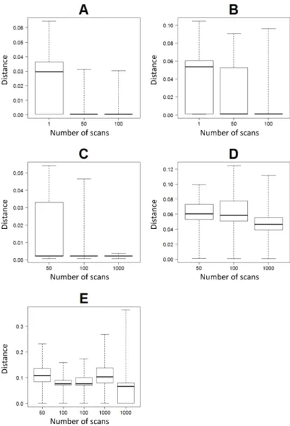
3.2. Results
For both distances and for each set of stratigraphic correlation parameters, the min-imum and maxmin-imum values, the first, second and third quartiles, were computed. The results are presented as box plots in Fig. 10 and 11 for the well distance and global distance respectively. These box plots summarize the full table of results provided in Appendix C.
For the same number of wells and scans in the training model, the data configurations A and B show lower distances than C and D respectively. A and B being almost as wide as the training model, the scan area is very constrained, allowing better correlations to be found more easily.
Surprisingly, by comparing A with B, and C with D, we can see that adding wells to constrain the model tends to increase the distances for the same number of scans. We need more scans to converge toward a distance equal to 0. It might be due to the fact that
Figure 10: Well distance box plots for each data configuration (Fig.8), for 100 realizations of correlations with different numbers of scans in the training model (number of positions of the data event that are tested). The well distance is a difference of relative geological time between the training model and the model realized from the correlation of the wells, at the position of this wells, see Eq. 5.
Figure 11: Global distance box plots for each data configuration (Fig.8), for 100 realizations of correla-tions with different numbers of scans in the training model (number of posicorrela-tions of the data event that are tested). The global distance is a difference of relative geological time between the training model and the model realized from the correlation of the wells, at nine positions regularly sampled in the model, see Eq. 5.
it is more difficult to find an optimal case, the number of scans being still a fraction of the total number of positions in the model, as there are more data to honor. Moreover, more wells involved in the correlation implies more possible stratigraphic correlations (Lallier et al., 2016). It may also be caused by the order chosen to do the correlations, which correlates closer wells first. There should be less variability between close wells than between wells that are far one from another. As a consequence, minor errors when correlating nearby wells can have large impact on the whole correlation.
For each data configuration, increasing the number of scans tends to decrease the global and the well distance medians. For E, a pair of sets of 100 correlations was computed for 100 and 1000 scans. We can see that the results are quite similar for 100 scans, but differ between the two sets of 1000 scans, one of them having a median being higher than for 50 scans. This might be also due to the order of correlation of the wells. The first well of the correlation varying, the data that have to be honored and the propagation of the errors during the correlation of the other wells may differ.
Fig. 11 shows about the same trends as Fig. 10. The statistics vary in detail, because spatial interpolation of strata away from wells can either increase or decrease the distance, depending on data layout. This highlights that the interpolation is sensitive to small variations between realizations that have the same well distance. In other words, two correlations that would only differ from the reference by one line may have the same well distances, but different global distances, because interpolation may increase the impact of small changes at data location. So, despite Fig. 10B-C showing statistical collapses for 100 scans, Fig. 11B-C proves that the models vary slightly from each other and that the method explores local uncertainties for a given correlation order of the wells. 3.3. Volumes
The volumes of the different units of the output models were also computed. Fig. 12 draws the cumulative volumes against relative geological time for models built from the stratigraphic correlation of the wells of the data configuration B, with 1, 50, and 100 scans in the training model. The comparison of these volumes shows the areas which are most uncertain. With a few scans, there are a lot of different paths, whereas with more scans, the curves are smoother, showing that patterns can be found when the training model is scanned thoroughly. The sum of all the curves seems less blurry, the global trend
Figure 12: Cumulative volumes of the 100 realizations per relative geological time (unit index / total number of units), built from the correlations of the wells B on Fig. 8, for different numbers of scans in the training model. The blue curve is the cumulative volumes of the training model rebuilt from the wells used in the data configuration B. Increasing the number of scans increases the chances to find the most probable associations, and so, decreases the number of possible paths in these graphs.
is more easily observable, and tends to follow the cumulative volumes of the training model rebuilt. In the case presented on Fig. 12, the correlations that do not reflect the training model, the ones that deviate from the blue line, tend to underestimate the volumes at the bottom of the wells and consequently overestimate the volumes at their top. This effect could be due to geometric interpolation artifacts as relative thicknesses are considered and must sum up to one (Mallet, 2002). Adapting compositional data interpolation methods (e.g., van den Boogaart et al. (2017); Walvoort and de Gruijter (2001)) could be an interesting perspective to address this bias.
3.4. Discussion and perspectives
The proposed method allows to build different possible models from a set of well data and is able to recover the same layer connectivity as the reference model from only a few wells. As the global stratigraphic column is rebuilt for each realization, the 3D architectures can be reconstructed by interpolation, showing similar relative volume trends as in the reference model. However several aspects of the method can be discussed. Data
Our method requires a training model to evaluate the likelihood of existence of as-sociation of units. It implies that this model and the well data to correlate not only
should share the same type of measurements (facies, logs) but also that they should be coherent. The training model must be a good representation of the units and geometry that can exist. This means that the model should present a similar environment as the environment in which the sediment sampled by the wells were deposited.
In this paper, we used a numerical model as training model to compute correlation costs, but natural analog models (Colombera et al., 2012) providing the same information as available well data could also be investigated. Indeed, the training model and the well data must bear the same property, to be able to compare their units. This property could be interpreted (e.g., facies), from raw measures (e.g., gamma ray, sonic, density). The method relies on the identification of stratigraphic sequences on the well data and in the forward model. Therefore, the resolution of the stratigraphic sequences (meaning the stratigraphic order of the units) should be the same on the wells and in the model. Also, the resolution of the property measured on the wells and in the training model should be comparable. As mistakes at this interpretation step are likely to have an impact on the output correlation, uncertainties should be accounted for. For example, the sequence interpretation of available wells by several experts could be considered for subsequent testing.
Moreover, as the depositional environment may vary within the analog model, the training model is not stationary. Stationarity is a known problem in classical Multiple-Points Statistic studies (e.g., Caers and Zhang (2002); Strebelle and Zhang (2005); Mirowski et al. (2009)). By default, the training image must show a stationary sta-tistical distribution, a stationary orientation, and a stationary scale (Mirowski et al., 2009). Here, the first requirement is not fulfilled : the deposits show a clear trend from proximal to distal. The information of distality could, therefore, be used as secondary variable, to help to account for the orientation, as proposed by Strebelle and Zhang (2005). The distality could also be discretized to split the training model into different zones to sample the corresponding information, as de Vries et al. (2009) suggest.
Finally, the area covered by the training model should be wider than the one covered by the well data to allow the search for correlation, using the data configuration, in different places. In our case, the data configuration A showed good results while being almost as wide as the training model but we knew a priori that it was at the right place
in the training model. Method and algorithm
We have seen that the average distances increase with the number of wells involved in the correlation, and that they can increase with the number of scans too, depending on the order of correlation of the wells. This stems from the combinatorial complexityof the correlation problem. Indeed, the number of possible correlations increases with the complexity of the data configuration (Lallier et al., 2016). In turn, it is more difficult to find a matching pattern in the training model, and the errors occuring at the correlation of the first wells are propagated to the correlation of the last wells. Moreover, these errors differ depending on the order of correlation of the wells. Different strategies can be considered to manage this problem.
First, the uncertainty space could be explored, by changing the order of correlation of the wells for each realization. Second, the method can be optimized. Lallier et al. (2016) propose to destroy and rebuild the correlations between wells sequentially, to take more recent correlations into account. Alternatively, Wheeler (2015) suggests to use a global alignment optimization postprocessing. Third, a multi-scale approach could be considered, as the multiple grid concept used in MPS methods (Tran, 1994; Strebelle, 2002; Liu, 2006; Hu and Chugunova, 2008). The wells that are far from each other could be correlated before precising the stratigraphic column with intermediate wells. In a similar way, the stratigraphic sequences along the wells could be considered in function of their stratigraphic order, by correlating high stratigraphic order before low orders, as suggested by Lallier et al. (2016).
Case study
We chose to focus on only a few parameters in this case study to analyze the method features. Further analysis should definitely be made by assessing the sensitivity of results to variations of other parameters like α and β in Eq. 3, or the costs of the rule used to compare a unit on a well with one in the model, for example.
The comparison cost functions p and t comparing well data and analog data in Eq. 1 and Eq. 3 could also be adapted to consider the history of the basin and to create coherent units successions in the correlation. For example, the cost computation of the association or the hiatus could account for the units above and below (instead of
comparing only below a gap). Moreover this rule could be associated with other rules to account for other geological concepts.
The forward model used in this study was very simple, and the method efficiency on more complex models should be investigated.
More fundamentally, a variety of sedimentary variables are produced by process-based simulations. We believe the proposed method could be used to test which parameters (or combination of parameters) best retrieves the stratigraphic architectures from a set of wells in a given depositional context.
After testing the sensitivity of the method, it should be tested on real data. One difficulty with applying this method to field data is generating a training model that is analog to the area of interest. However, a quick study of the data available can give large scale information such as sediment source or global change of sea level. If uncertainties remain, several forward models can be built to sample these uncertainties, and then they can be used as training models for the stratigraphic correlation of the well data. Results
The variations between the resulting correlations, translated in the curves of cumu-lative volumes, are due to the different positions of gaps, interpreted as pinch-outs of the horizons due to erosions or non-deposition. They make the sedimentation rates vary locally, with a different distribution of the sediments and hiatuses during time (vertically in the model).
The sedimentation rate and the role of unconformities in the stratigraphic record have profound implications in basin studies, to understand source-to-sink processes and the coupling between climate and tectonics (Molnar and England, 1990; M´etivier et al., 1999; Zhang et al., 2001; Molnar, 2004; Clift, 2006; Charreau et al., 2011; Herman and Cham-pagnac, 2016; Willenbring and Jerolmack, 2016; Bhattacharya et al., 2016). Because no mass is lost in the process of erosion, transport and sedimentation, sedimentary basins provide key archives to reconstruct the paleo denudation rates (e.g. Hay et al. (1989); Dromart et al. (2002); Rouby et al. (2009); Guillocheau et al. (2012); Nicholson et al. (2016)). We believe the method proposed in this paper could help providing some lower bounds for the distribution of hiatuses in the sediment record. A sensitivity study on the gap cost and further work integrating recent discussions on the sedimentation rate and
the distribution and meaning of gaps (Sadler, 1999; Sadler and Jerolmack, 2014; Miall, 2016; Tipper, 2016) are, therefore, important perspectives of this work.
The differences of volumes distribution may also have a high impact on reservoir studies, especially for the computation of fluid volumes and fluid flow (Jackson et al., 2009; Lallier et al., 2012; Cavero et al., 2016). Indeed, the position of pinch-outs can be critical for reservoir compartmentalization.
In this work, we used a deterministic method to build 3D models honoring the corre-lations and the associated stratigraphic column. In practice, significant uncertainty may exist due to the lack of data, so methods to simulate possible stratigraphic geometries should also be considered (Goff, 2000; Abrahamsen et al., 1992; Caumon, 2010; Cherpeau and Caumon, 2015). Indeed, when the algorithm outputs a hiatus, there is no clue to identify the position of the hiatus (for example the erosion line) between the wells. This line could be drawn in a range of possible positions. The lateral thickness variation of the units between the wells, or equivalently the geometry of the bottom and top horizons of this unit, is also unknown and could be simulated.
Conclusions
We presented in this paper a method to output stochastic stratigraphic models, in-cluding the geometry of the units of the area covered by the wells and their respective topological relationships.
This is possible by building the stratigraphic column of the area during the correlation of the well data. Indeed, the stratigraphic correlation of the wells is made by correlating their corresponding stratigraphic columns, and updating the global stratigraphic column after each addition of a well to the previous correlation.
The algorithm used is the Dynamic Time Warping with a single rule. The rule consists in computing the likelihood of each association of units by searching for their occurrences in a training model built with forward modeling methods.
The method has been tested on synthetic data and gives quite coherent results but highlights the challenges to explore the space of possible models. Further work includes making sensitivity analysis of the different parameters, studying the impact of the cor-relation order of the wells, and applying the method on real data.
Acknowledgments
This work was performed in the frame of the RING project at Universit´e de Lorraine. We would like to thank for their support the industrial and academic sponsors of the RING-GOCAD Consortium managed by ASGA. We also acknowledge Paradigm for the SKUA-Gocad Software and API. Software corresponding to this paper is available to sponsors in the RING software package SCube.
Abrahamsen, P., Lia, O., Omre, H., et al., 1992. An integrated approach to prediction of hydrocar-bon in place and recoverable reserve with uncertainty measures. In: European Petroleum Computer Conference. Society of Petroleum Engineers.
Agterberg, F., Gradstein, F., Cheng, Q., Liu, G., 2013. The RASC and CASC programs for ranking, scaling and correlation of biostratigraphic events. Computers & Geosciences 54, 279–292.
Agterberg, F. P., 1990. Automated Stratigraphic Correlation. Developments in Palaeontology and Stratigraphy. Elsevier.
Armitage, J. J., Allen, P. A., Burgess, P. M., Hampson, G. J., Whittaker, A. C., Duller, R. A., Michael, N. A., 2015. Sediment transport model for the Eocene Escanilla sediment-routing system: Implications for the uniqueness of sequence stratigraphic architectures. Journal of Sedimentary Research 85 (12), 1510–1524.
Bhattacharya, J. P., Copeland, P., Lawton, T. F., Holbrook, J., 2016. Estimation of source area, river paleo-discharge, paleoslope, and sediment budgets of linked deep-time depositional systems and im-plications for hydrocarbon potential. Earth-Science Reviews 153, 77–110.
Borgomano, J. R. F., Fourrier, F., Viseur, S., Rijkels, L., 2008. Stratigraphic well correlations for 3D static modeling of carbonate reservoirs. AAPG Bulletin 92, 789–824.
Brown, I. M., 1997. A new method for correlation of multiple stratigraphic sequences. Computers and Geosciences 23, 697–700.
Burbank, D. W., Leland, J., Fielding, E., Anderson, R. S., Brozovic, N., Reid, M. R., Duncan, C., 1996. Bedrock incision, rock uplift and threshold hillslopes in the northwestern himalayas. Nature 379 (6565), 505–510.
Burgess, P. M., 2012. A brief review of developments in stratigraphic forward modelling, 2000–2009. Regional Geology and Tectonics: Principles of Geologic Analysis, 378–404.
Burgess, P. M., Prince, G. D., 2015. Non-unique stratal geometries: implications for sequence strati-graphic interpretations. Basin Research 27 (3), 351–365.
Caers, J., Zhang, T., 2002. Multiple-point geostatistics: a quantitative vehicle for integrating geologic analogs into multiple reservoir models.
Catuneanu, O., Willis, A. J., Miall, A. D., 1998. Temporal significance of sequence boundaries. Sedi-mentary Geology 121 (3), 157–178.
Caumon, G., 2010. Towards stochastic time-varying geological modeling. Mathematical Geosciences 42 (5), 555–569.
Caumon, G., Journel, A. G., 2005. Early uncertainty assessment: Application to a hydrocarbon reservoir appraisal. Geostatistics Banff 2004, 551–557.
Cavero, J., Orellana, N., Yemez, I., Singh, V., Izaguirre, E., 2016. Importance of conceptual geological models in 3D reservoir modelling. First Break 34 (7), 39–49.
Charreau, J., Blard, P.-H., Puchol, N., Avouac, J.-P., Lallier-Verges, E., Bourl`es, D., Braucher, R., Gallaud, A., Finkel, R., Jolivet, M., et al., 2011. Paleo-erosion rates in Central Asia since 9Ma: A transient increase at the onset of Quaternary glaciations? Earth and Planetary Science Letters 304 (1), 85–92.
Charvin, K., Gallagher, K., Hampson, G. L., Labourdette, R., 2009. A bayesian approach to inverse modelling of stratigraphy, part 1: Method. Basin Research 21 (1), 5–25.
Cherpeau, N., Caumon, G., 2015. Stochastic structural modelling in sparse data situations. Petroleum Geoscience 21 (4), 233–247.
Clift, P. D., 2006. Controls on the erosion of Cenozoic Asia and the flux of clastic sediment to the ocean. Earth and Planetary Science Letters 241 (3), 571–580.
con-straining stochastic simulations of the sedimentary heterogeneity of fluvial reservoirs. AAPG Bulletin 96 (11), 2143–2166.
Cross, T. A., Lessenger, M. A., 1999. Construction and application of a stratigraphic inverse model. In: Harbaugh, J. W., Watney, W. L., Rankey, E. C., Slingerland, R., Goldstein, R. H., , Franseen, E. K. (Eds.), Numerical Experiments in Stratigraphy: Recent Advances in Stratigraphic and Sedimentologic Computer Simulations. Vol. 62. SEPM, Special Publications, p. 69–83.
de Vries, L. M., Carrera, J., Falivene, O., Gratac´os, O., Slooten, L. J., 2009. Application of multiple point geostatistics to non-stationary images. Mathematical Geosciences 41 (1), 29–42.
Dromart, G., Garcia, J.-P., Allemand, P., Gaumet, F., Rousselle, B., 2002. A volume-based approach to calculation of ancient carbonate accumulations. The Journal of geology 110 (2), 195–210.
Embry, A. F., 2002. Transgressive-regressive (TR) sequence stratigraphy. In: Gulf Coast SEPM Confer-ence Proceedings, Houston. SEPM, pp. 151–172.
Falivene, O., Frascati, A., Gesbert, S., Pickens, J., Hsu, Y., Rovira, A., Sep 2014. Automatic calibration of stratigraphic forward models for predicting reservoir presence in exploration. AAPG Bulletin 98 (9), 1811–1835.
Fang, J. H., Chen, H. C., Shultz, A. W., Mahmoud, W., 1992. Computer-aided well log correlation. AAPG Bulletin 76 (3), 307–317.
Gari, J., 2007. Mod´elisation stratigraphique haute r´esolution 3D de syst`emes s´edimentaires carbonat´es: les affleurements de la marge carbonat´ee du Beausset d’ˆage C´enomanien `a Coniacien moyen (Provence, France). Ph.D. thesis, Universit´e de Provence, Marseille, France.
Goff, J. A., 2000. Simulation of stratigraphic architecture from statistical and geometrical characteriza-tions. Mathematical Geology 32 (7), 765–786.
Gordon, A. D., Reyment, R. A., 1979. Slotting of borehole sequences. Journal of the International Association for Mathematical Geology 11 (3), 309–327.
Granjeon, D., 1997. Mod´elisation stratigraphique d´eterministe: conception et applications d’un mod`ele diffusif 3D multilithologique. Ph.D. thesis, Universit´e de Rennes.
Guardiano, F. B., Srivastava, R. M., 1993. Multivariate geostatistics: beyond bivariate moments. In: Geostatistics Troia’92. Springer, pp. 133–144.
Guillocheau, F., Rouby, D., Robin, C., Helm, C., Rolland, N., Le Carlier de Veslud, C., Braun, J., 2012. Quantification and causes of the terrigeneous sediment budget at the scale of a continental margin: a new method applied to the Namibia–South Africa margin. Basin Research 24 (1), 3–30.
Harris, P. M., Kenter, J., Playton, T., Andres, M., Jones, G., Levy, M., 2011. Enhancing subsurface reservoir models – an integrated MPS approach using outcrop analogs, modern analogs, and forward stratigraphic models. In: Annual Convention and Exhibition. AAPG, Houston, Texas, USA, April 10-13.
Hay, W. W., Shaw, C. A., Wold, C. N., 1989. Mass-balanced paleogeographic reconstructions. Geologis-che Rundschau 78 (1), 207–242.
Helland-Hansen, W., Gjelberg, J. G., 1994. Conceptual basis and variability in sequence stratigraphy: a different perspective. Sedimentary Geology 92 (1), 31–52.
Herman, F., Champagnac, J.-D., 2016. Plio-Pleistocene increase of erosion rates in mountain belts in response to climate change. Terra Nova 28 (1), 2–10.
Howell, J. A., 1983. A fortran 77 program for automatic stratigraphic correlation. Computers and Geo-sciences 9 (3), 311–327.
Hu, L., Chugunova, T., 2008. Multiple-point geostatistics for modeling subsurface heterogeneity: A comprehensive review. Water Resources Research 44 (11).
Jackson, M. D., Hampson, G. J., Sech, R. P., 2009. Three-dimensional modeling of a shoreface-shelf parasequence reservoir analog: Part 2. geologic controls on fluid flow and hydrocarbon recovery. AAPG Bulletin 93 (9), 1183–1208.
Journel, A. G., Bitanov, A., 2004. Uncertainty in n/g ratio in early reservoir development. Journal of Petroleum Science and Engineering 44 (1), 115–130.
Kendall, C. S. C., Strobel, J., Cannon, R., Bezdek, J., Biswas, G., 1991. The simulation of the sedimen-tary fill of basins. Journal of Geophysical Research: Solid Earth 96 (B4), 6911–6929.
Koehrer, B., Aigner, T., P¨oppelreiter, M., 2011. Field-scale geometries of Upper Khuff reservoir geobodies in an outcrop analogue (Oman mountains, Sultanate of Oman). Petroleum Geoscience 17 (1), 3–16. Lallier, F., Caumon, G., Borgomano, J., Viseur, S., Fournier, F., Antoine, C., Gentilhomme, T., 2012.
Relevance of the stochastic stratigraphic well correlation approach for the study of complex carbonate settings: application to the Malampaya buildup (offshore Palawan, Philippines). Geological Society, London, Special Publications 370 (1), 265–275.
as-sessment in the stratigraphic well correlation of a carbonate ramp: Method and application to the Beausset Basin, SE France. Comptes Rendus Geoscience 348, 499–509.
Lallier, F., Viseur, S., Borgomano, J., Caumon, G., et al., 2009. 3D stochastic stratigraphic well corre-lation of carbonate ramp systems. In: International Petroleum Technology Conference. International Petroleum Technology Conference.
Lawrence, D. T., Doyle, M., Aigner, T., 1990. Stratigraphic simulation of sedimentary basins: Concepts and calibration (1). AAPG Bulletin 74 (3), 273–295.
Levenshtein, V., 1966. Binary codes capable of correcting deletions, insertions, and reversals. Soviet Physics-Doklady 10 (8), 707–710.
Liu, Y., 2006. Using the Snesim program for multiple-point statistical simulation. Computers & Geo-sciences 32 (10), 1544–1563.
Mallet, J.-L., 2002. Geomodeling. Oxford University Press.
Mariethoz, G., Renard, P., Straubhaar, J., 2010. The Direct Sampling method to perform multiple-point geostatistical simulations. Water Resources Research 46 (11).
Massonnat, G., Pernarcic, E., et al., 2002. NEPTUNE: An innovative approach to significantly improve reservoir modeling in carbonate reservoirs. In: Abu Dhabi International Petroleum Exhibition and Conference. Society of Petroleum Engineers.
M´etivier, F., Gaudemer, Y., Tapponnier, P., Klein, M., 1999. Mass accumulation rates in Asia during the Cenozoic. Geophysical Journal International 137 (2), 280–318.
Miall, A. D., 2016. The valuation of unconformities. Earth-Science Reviews 163, 22–71.
Mirowski, P. W., Tetzlaff, D. M., Davies, R. C., McCormick, D. S., Williams, N., Signer, C., 2009. Stationarity scores on training images for multipoint geostatistics. Mathematical geosciences 41 (4), 447–474.
Molnar, P., 2004. Late Cenozoic increase in accumulation rates of terrestrial sediment: how might climate change have affected erosion rates? Annu. Rev. Earth Planet. Sci. 32, 67–89.
Molnar, P., England, P., 1990. Late enozoic uplift of mountain ranges and global climate change: chicken or egg? Nature 346 (6279), 29–34.
Myers, C. S., Rabiner, L. R., 1981. Comparative study of several dynamic time warping algorithms for connected-word recognition. The Bell System Technical Journal 60 (7), 1389–1409.
Nakagawa, S., Nakanishi, H., 1988. Speaker-independent English consonant and Japanese word recog-nition by a stochastic dynamic time warping method. Journal of the Institution of Electronics and Telecommunication Engineers 34 (1), 87–95.
Nicholson, U., Es, B., Clift, P. D., Flecker, R., Macdonald, D. I., 2016. The sedimentary and tectonic evolution of the Amur River and North Sakhalin Basin: new evidence from seismic stratigraphy and Neogene–Recent sediment budgets. Basin Research.
Olea, R. A., 1994. Expert systems for automated correlation and interpretation of wireline logs. Mathe-matical Geology 26 (8), 879–897.
Olea, R. A., 2004. Correlator 5.2 - a program for interactive lithostratigraphic correlation of wireline logs. Computers and Geosciences 30 (6), 561–567.
Pels, B., Keizer, J. J., Young, R., 1996. Automated biostratigraphic correlation of palynological records on the basis of shapes of pollen curves and evaluation of next-best solutions. Palaeogeography, Palaeo-climatology, Palaeoecology 124, 17–37.
Rouby, D., Bonnet, S., Guillocheau, F., Gallagher, K., Robin, C., Biancotto, F., Dauteuil, O., Braun, J., 2009. Sediment supply to the Orange sedimentary system over the last 150My: An evaluation from sedimentation/denudation balance. Marine and Petroleum Geology 26 (6), 782–794.
Sacchi, Q., Borello, E. S., Weltje, G. J., Dalman, R., 2016. Increasing the predictive power of geosta-tistical reservoir models by integration of geological constraints from stratigraphic forward modeling. Marine and Petroleum Geology 69, 112–126.
Sacchi, Q., Weltje, G. J., Verga, F., Mar 2015. Towards process-based geological reservoir modelling: Obtaining basin-scale constraints from seismic and well data. Marine and Petroleum Geology 61, 56–68.
Sadler, P., 1999. The influence of hiatuses on sediment accumulation rates. In: GeoResearch Forum. Vol. 5.
Sadler, P. M., Jerolmack, D. J., 2014. Scaling laws for aggradation, denudation and progradation rates: the case for time-scale invariance at sediment sources and sinks. Geological Society, London, Special Publications 404 (1), 69–88.
Sakoe, H., Chiba, S., 1978. Dynamic programming algorithm optimization for spoken word recognition. IEEE transactions on acoustics, speech, and signal processing 26 (1), 43–49.
88 (4), 451–457.
Strebelle, S., 2002. Conditional simulation of complex geological structures using multiple-point statistics. Mathematical Geology 34 (1), 1–21.
Strebelle, S., Zhang, T., 2005. Non-stationary multiple-point geostatistical models. Geostatistics Banff 2004, 235–244.
Tetzlaff, D. M., Harbaugh, J. W., 1989. Simulating clastic sedimentation. Computer Methods in the Geosciences. Springer.
Tipper, J. C., 2016. Measured rates of sedimentation: What exactly are we estimating, and why? Sedimentary Geology 339, 151–171.
Tran, T. T., 1994. Improving variogram reproduction on dense simulation grids. Computers & Geo-sciences 20 (7-8), 1161–1168.
van den Boogaart, K. G., Mueller, U., Tolosana-Delgado, R., 2017. An affine equivariant multivariate normal score transform for compositional data. Mathematical Geosciences 49 (2), 231–251.
Walvoort, D. J., de Gruijter, J. J., 2001. Compositional kriging: a spatial interpolation method for compositional data. Mathematical Geology 33 (8), 951–966.
Waterman, M. S., Raymond, R., 1987. The match game: New stratigraphic correlation algorithms. Mathematical Geology 19 (2), 109–127.
Wheeler, H. E., 1958. Time-stratigraphy. AAPG Bulletin 42 (5), 1047–1063.
Wheeler, L. F., 2015. Automatic and simultaneous correlation of multiple well logs. Colorado School of Mines.
Willenbring, J. K., Jerolmack, D. J., 2016. The null hypothesis: globally steady rates of erosion, weath-ering fluxes and shelf sediment accumulation during Late Cenozoic mountain uplift and glaciation. Terra Nova 28 (1), 11–18.
Wingate, D., Kane, J., Wolinsky, M., Sylvester, Z., 2016. A new approach for conditioning process-based geologic models to well data. Mathematical Geosciences 48 (4), 371–397.
Zhang, P., Molnar, P., Downs, W. R., 2001. Increased sedimentation rates and grain sizes 2–4 Myr ago due to the influence of climate change on erosion rates. Nature 410 (6831), 891–897.
Appendix A. Dynamic Time Warping
The Dynamic Time Warping (DTW) algorithm is an effective algorithm to correlate two sequences using a set of rules. Initially developed for speech recognition, it has been used in many fields (video, audio, graphics, bioinformatics) (Levenshtein, 1966; Sakoe and Chiba, 1978; Myers and Rabiner, 1981; Howell, 1983; Waterman and Raymond, 1987). The rules are used to compute a cost of correlation for each pair of elements independently. The most probable correlation of the two series, following the rules given, will be the one with the global minimum cost. DTW was first used for stratigraphic correlation by Smith and Waterman (1980).
The cost can be represented in a table (Fig. A.13). A cell (i, j) in the table repre-sents a correlation between the two corresponding markers i and j of the wells 1 and 2, respectively. There are different ways to move in the table from a cell to another. An oblique transition corresponds to a correlation between two units. A vertical or horizon-tal transition shows gaps (a unit observed on a well is absent on the other well). The table is filled from the bottom left cell (1, 1) to the top right cell (n, m).
Figure A.13: Cost table of the Dynamic Time Warping algorithm. n and m are the number of markers of the wells 1 and 2 respectively. c(i,j) is the cost of the correlation of the markers i and j. The three
arrows are the transitions available: the horizontal and vertical transitions are gaps tj,ji,i−1and tj,j−1i,i respectively, and the diagonal transition is a match tj,j−1i,i−1.
Model length 100 km Model width 100 km Cell length 0.5 km Cell width 0.5 km Timespan 70 My Time step 0.2 My
Table B.1: Model dimensions in time and space.
The cumulative costs C(i,j) are computed following the recursive formula (Lallier
et al., 2009): C(i,j)= min tj,j−1i,i−1 + C(i−1,j−1) tj,ji,i−1+ C(i−1,j) tj,j−1i,i + C(i,j−1) (A.1)
The three members in brackets are the costs for three possible transitions, two gaps (tj,j−1i,i−1, tj,j−1i,i ) and a match (tj,ji,i−1), see Fig. A.13. The cost of the previous cell in each case is added, so that C(i, j) stands for the cumulative cost of the two units, i from the first well, and j from the second well, and all the previous associations in the path. This recursive formula ensures that the global minimum cost is found. Finally, the path in the table with minimum cost is retrieved by local propagation from the upper right (n, m) cell, representing the best correlation.
The DTW has been modified by several authors to implement a stochastic version of the algorithm (Nakagawa and Nakanishi, 1988; Pels et al., 1996). A possibility to reflect uncertainties of the cost computation is to randomly sample the propagation in the cost matrix (Lallier et al., 2009).
Appendix B. Dionisos model characteristics
The model dimensions are shown in table B.1. The initial topography of the sea floor follows the map shown in Fig. B.14 and the simulation runs for 70 My. The sediment input rate is constant and equals 20 km3 per My. The eustasy variation is shown on Fig. B.16. There is a global subsidence making the basement topography to be lowered by 120m during the whole timespan. The resulting cell’s average thickness is about 1m (Fig. B.15).
Figure B.14: Bathymetry (m) of the basement at t=0 (vertical exaggeration: x150).
4 6 8 10 0 10 20 30 40 50 60 70 Sea Level (m) Age (My)
Appendix C. Distances between the models from the correlation results and the training model
The table C.2 presents the global distance and well distance of the sets of stratigraphic correlations, for the different data configurations seen on Fig. 8, and different number of scans in the training model.
Data configuration A B C Scans 1 50 100 1 50 100 50 100 1000 Min 0.00 0.00 0.00 0.00 0.00 0.00 0.02 0.02 0.02 Global P25 0.00 0.00 0.00 0.001 0.01 0.01 0.06 0.06 0.06 P50 0.05 0.00 0.00 0.15 0.01 0.01 0.06 0.06 0.06 distance P75 0.13 0.00 0.00 0.20 0.17 0.02 0.18 0.07 0.06 Max 0.27 0.04 0.07 0.26 0.26 0.27 0.61 0.60 0.13 Min 0.00 0.00 0.00 0.00 0.00 0.00 0.00 0.00 0.00 Well P25 0.00 0.00 0.00 0.00 0.00 0.00 0.01 0.01 0.01 P50 0.13 0.00 0.00 0.10 0.00 0.00 0.01 0.01 0.01 distance P75 0.15 0.00 0.00 0.11 0.10 0.00 0.14 0.01 0.01 Max 0.27 0.13 0.13 0.20 0.17 0.18 0.23 0.20 0.02 Data configuration D E Scans 50 100 1000 50 100 100 1000 1000 Min 0.03 0.03 0.03 0.03 0.03 0.03 0.02 0.03 Global P25 0.12 0.09 0.06 0.13 0.11 0.10 0.04 0.13 P50 0.38 0.32 0.10 0.15 0.12 0.13 0.09 0.16 distance P75 0.43 0.38 0.14 0.17 0.14 0.15 0.12 0.20 Max 0.55 0.53 0.55 0.30 0.23 0.24 0.41 0.33 Min 0.00 0.00 0.00 0.00 0.00 0.00 0.00 0.00 Well P25 0.10 0.10 0.07 0.08 0.07 0.07 0.08 0.00 P50 0.11 0.11 0.09 0.11 0.08 0.08 0.10 0.07 distance P75 0.14 0.15 0.11 0.14 0.09 0.10 0.14 0.08 Max 0.19 0.24 0.21 0.23 0.16 0.17 0.27 0.36
Table C.2: Minimum, first, second and third quartiles, and maximum of the global distance and the well distance between the models realized and the training model (rebuilt using corresponding well data) for 100 realizations of stratigraphic correlations, for different numbers of scans in the training model, and different wells used for the correlation (A, B, C, D, E correspond to the positions of the wells on the data configurations shown on Fig. 8).