HAL Id: hal-01117347
https://hal.archives-ouvertes.fr/hal-01117347
Submitted on 20 Feb 2015
HAL is a multi-disciplinary open access
archive for the deposit and dissemination of
sci-entific research documents, whether they are
pub-lished or not. The documents may come from
teaching and research institutions in France or
abroad, or from public or private research centers.
L’archive ouverte pluridisciplinaire HAL, est
destinée au dépôt et à la diffusion de documents
scientifiques de niveau recherche, publiés ou non,
émanant des établissements d’enseignement et de
recherche français ou étrangers, des laboratoires
publics ou privés.
from space observation using ACE-FTS solar occultation
instrument
P. Y. Foucher, A. Chedin, R. Armante, C. Boone, C. Crevoisier, P. Bernath
To cite this version:
P. Y. Foucher, A. Chedin, R. Armante, C. Boone, C. Crevoisier, et al.. Carbon dioxide
atmo-spheric vertical profiles retrieved from space observation using ACE-FTS solar occultation
instru-ment. Atmospheric Chemistry and Physics, European Geosciences Union, 2011, 11 (6), pp.2455-2470.
�10.5194/acp-11-2455-2011�. �hal-01117347�
www.atmos-chem-phys.net/11/2455/2011/ doi:10.5194/acp-11-2455-2011
© Author(s) 2011. CC Attribution 3.0 License.
Chemistry
and Physics
Carbon dioxide atmospheric vertical profiles retrieved from space
observation using ACE-FTS solar occultation instrument
P. Y. Foucher1,2, A. Ch´edin1, R. Armante1, C. Boone3, C. Crevoisier1, and P. Bernath3,4
1Laboratoire de M´et´eorologie Dynamique/Institut Pierre Simon Laplace, Ecole Polytechnique, 91128 Palaiseau, France
2Onera – The French Aerospace Lab, Centre Midi-Pyr´en´ees, 31055 Toulouse Cedex 4, France
3Department of Chemistry, University of Waterloo, Ontario, N2L3G1, Canada
4Department of Chemistry, University of York, Heslington, York, YO105DD, UK
Received: 9 August 2010 – Published in Atmos. Chem. Phys. Discuss.: 5 November 2010 Revised: 25 February 2011 – Accepted: 8 March 2011 – Published: 16 March 2011
Abstract. Major limitations of our present knowledge of
the global distribution of CO2in the atmosphere are the
un-certainty in atmospheric transport and the sparseness of in situ concentration measurements. Limb viewing spaceborne sounders such as the Atmospheric Chemistry Experiment Fourier transform spectrometer (ACE-FTS) offer a vertical resolution of a few kilometres for profiles, which is much better than currently flying or planned nadir sounding instru-ments can achieve. After having demonstrated the
feasibil-ity of obtaining CO2vertical profiles in the 5–25 km altitude
range with an accuracy of about 2 ppm in a previous study, we present here the results of five years of ACE-FTS
observa-tions in terms of monthly mean profiles of CO2averaged over
10◦latitude bands for northern mid-latitudes. These results
are compared with in-situ aircraft measurements and with simulations from two different air transport models. Key
fea-tures of the measured altitude distribution of CO2are shown
to be accurately reproduced by the ACE-FTS retrievals: vari-ation in altitude of the seasonal cycle amplitude and extrema, seasonal change of the vertical gradient, and mean growth rate. We show that small but significant differences from model simulations could result from an over estimation of the model circulation strength during the northern hemisphere spring. Coupled with column measurements from a nadir viewing instrument, it is expected that occultation measure-ments will bring useful constraints to the surface carbon flux determination.
Correspondence to: P. Y. Foucher
(pierre-yves.foucher@lmd.polytechnique.fr)
1 Introduction
Determining the spatial and temporal structure of surface car-bon fluxes has become a major scientific goal during the last decade. In the so-called ”inverse” approach, observed atmo-spheric concentration gradients are used to disentangle sur-face fluxes, given some description of atmospheric transport. Major limitations of the inverse approach are the
sparse-ness of atmospheric CO2 concentration measurements,
of-ten compensated for by introducing questionable constrain-ing conditions, and, more significantly, the uncertainties in
atmospheric transport. Since CO2 is inert in the lower
at-mosphere, its long-term trend and pronounced seasonal cycle propagate from the surface, and the difference between atmo-spheric and surface mixing ratios is determined by the pro-cesses that transport surface air throughout the atmosphere, including advection, convection and eddy mixing (Shia et al., 2006). Because it takes several months to transport surface
air to the lower stratosphere, the CO2mixing ratio is lower
and the seasonal cycle is different there as compared to the troposphere (Plumb and Ko, 1992; Plumb, 1996; Shia et al., 2006). B¨onisch et al. (2008) evaluated transport in three-dimensional chemical transport models in the upper tropo-sphere and lower stratotropo-sphere by using observed
distribu-tions of CO2and SF6. They show that although all models
are able to capture the general features in tracer distributions
including the vertical and horizontal propagation of the CO2
seasonal cycle, important problems remain such as: (i) a too strong Brewer-Dobson circulation (with air rising across the tropical tropopause, moving poleward, and sinking to the ex-tratropical troposphere) causing an overestimate of the tracer concentration in the lower most stratosphere (LMS) during
winter and spring and, (ii) a too strong tropical isolation lead-ing to an underestimate of the tracers in the LMS durlead-ing win-ter. Moreover, all models tested suffer to some extent from diffusion and/or too strong mixing across the tropopause. In addition, the models show too weak vertical upward trans-port into the upper troposphere during the boreal summer.
In recent years it has become possible to measure
atmo-spheric CO2 from space observations by the nadir-viewing
thermal infrared vertical sounders such as TIROS-N Op-erational Vertical Sounder (TOVS) (Ch´edin et al., 2002, 2003a), Atmospheric Infrared Sounder (AIRS), Infrared At-mospheric Sounder Interferometer (IASI) (Ch´edin et al., 2003b; Crevoisier et al., 2004, 2009) and Tropospheric Emis-sion Spectrometer (TES) instrument (Kulawik et al., 2010), or in the near infrared by SCIAMACHY (Buchwitz et al., 2005) and Greenhouse gases Observing SATellite (GOSAT) (Kuze et al., 2009). However, the satellite data products are all vertically integrated concentrations rather than the profile measurements that are essential for a comprehensive
under-standing of distribution mechanisms of CO2. The difference
between the column-averaged CO2mixing ratio and the
sur-face value varies from 2 to 10 ppm depending on location and time of year (Olsen and Randerson, 2004). The upper troposphere can contribute significantly to this difference be-cause this portion of the column constitutes approximately
20% of the column air mass and the CO2mixing ratios in
this region can differ by 5 ppm or more from the CO2mixing
ratios at the surface (Anderson et al., 1996; Matsueda et al., 2002; Shia et al., 2006). With limb sounders that observe the atmosphere along tangential optical paths, the vertical reso-lution of the measured vertical profiles is of the order of a few kilometres, much better than can be achieved with nadir sounding instruments. The Atmospheric Chemistry Experi-ment Fourier transform spectrometer (ACE-FTS), launched in August 2003 on board SCISAT, is a limb sounder that records solar occultation measurements (up to 30
occulta-tions each day) with coverage between approximately 85◦N
and 85◦S (Bernath et al., 2005), with more observations at
high latitudes than over the tropics (Bernath et al., 2006).
The ACE-FTS has high spectral resolution (0.02 cm−1) and
the signal-to-noise ratio of ACE-FTS spectra is higher than
300:1 over a large portion (1000–3000 cm−1) of the
spec-tral range covered (750–4400 cm−1). Recently, Foucher et
al. (2009) and Foucher (2009) have shown that the ACE-FTS
instrument is able to provide CO2vertical profiles in the
5-25 km altitude range with an estimated CO2total error
char-acterized by a bias of about ±1 ppm and a standard deviation of about 2 ppm after averaging over 20 spatially and tem-porally consistent retrieved profiles. Rinsland et al. (2010), using ACE-FTS and a method similar to that of Foucher et
al. (2009), have retrieved average dry air CO2 mole
frac-tions in the layer 7–10 km but did not extend their study to the retrieval of profiles. Beagley et al. (2010), again using
ACE-FTS, have retrieved CO2profiles in the mesosphere and
lower thermosphere where the problem of pointing
knowl-edge uncertainties is not a concern. Our analysis is organ-ised as follows. We first summarize the main features of the
method developed to retrieve CO2profiles and describe how
ACE-FTS occultations are selected (Sect. 2) and the limits of their spatial and temporal coverage. ACE-retrieved monthly
mean CO2vertical profiles averaged over the latitude bands
40◦N–60◦N and 50◦N–0◦N and covering the 2004–2008
time period are then presented and compared (vertical gradi-ents, seasonal cycles at various altitudes, growth rates) with aircraft in-situ measurements (Sect. 3) and with simulations from two different air transport models (Sect. 4). Section 5 presents our conclusions.
2 Method and ACE-FTS data
The methodology used to determine CO2profiles from
ACE-FTS observations has been described in detail in Foucher et al. (2009), hereafter referred to as Fal2009, and Foucher (2009). The retrieval process has two main steps: pointing parameter estimation (tangent heights, pressure and
temper-ature profiles) and CO2vertical profile estimation. Both steps
use a similar constrained least-squares retrieval method. The target variable is a vector containing tangent heights and a
temperature profile in the first step or a CO2 concentration
vertical profile in the second step.
2.1 ACE-FTS pointing knowledge
Interpreting limb viewing observations in terms of at-mospheric variables requires accurate knowledge of in-strument pointing parameters (tangent heights) and
pres-sure/temperature (”pT”) vertical profiles. Reactive trace
gases are the usual target species of limb-viewing instru-ments, so pointing parameters are simultaneously retrieved
with pT by the analysis of properly selected CO2lines
un-der the assumption (questionable, in certain cases) of a weak variation of its atmospheric concentration around a given a priori value. As carbon dioxide is here the target species, a critical step in this research has therefore been to develop a method of obtaining pT profiles and tangent heights
inde-pendent of any a priori CO2 knowledge. A new approach
based on the N2collision-induced continuum absorption near
4.3 µm was presented in Fal2009 together with a new
para-metric N2 continuum absorption model derived from
Laf-ferty et al. (1996) laboratory measurements. The high
sen-sitivity of N2continuum absorption to tangent height affords
a precision of better than 50 m in the tangent height retrieval.
Figure 1 shows N2 continuum transmittance sensitivity to
tangent height in the 2400–2600 cm−1 spectral range. As
explained in Fal2009, five optimized micro-windows were
selected in the 2400 to 2500 cm−1 wave number range in
order to cover the 5–25 km altitude range. Here, a new
micro-window near 2430 cm−1has been added to increase
N2transmittance sensitivity to altitude Wave number (cm-1) Altitude (km) ) ( * 1 . 0 −1 ∂ ∂ km z τ
Fig. 1. Transmittance sensitivity to tangent height in the N2
collision-induced absorption (2370–2640 cm−1) spectral range. The color bar values represent the transmission variation due to a 100 m tangent height change.
hydrostatic equilibrium we obtain ACE-FTS tangent heights
independent of a priori CO2data with a high precision (50 m
standard deviation). Finally, empirical corrections are added to these tangent heights to account for problems in the
trans-mission model which does not include effects of N2-H2O
collisions, which are still not accurately known. In addi-tion, although we included the latest developments in the modelling of line wings based on Niro et al. (2004), there
might still be uncertainties near 2400 cm−1. These empirical
corrections have been estimated based on the analysis of the mean difference between ACE v2.2 tangent heights (Boone
et al., 2005) and tangent heights retrieved from the N2
contin-uum, based on averages over the entire 2004–2008 time pe-riod. This mean bias depends on the altitude and varies from
−2.5% at lowest altitude to +2% at 20 km. This correction
is applied to all occultations and is described in more detail in Foucher et al. (2009). Using a method similar to that de-scribed in Foucher (2009), Rinsland et al. (2010) find
ACE-retrieved CO2mean tropospheric concentration for the layer
7–10 km around 405–420 ppm, too high by about 30 ppm.
This large bias is likely due to the use of an uncorrected N2
continuum absorption.
2.2 Selection of ACE-FTS occultations
A high inclination (74◦), circular, low Earth orbit (650 km)
gives ACE coverage of tropical, mid-latitude and polar gions. The ACE orbit was selected so that the coverage re-peats annually in latitude (Bernath et al., 2006) and is opti-mized for high latitude coverage in both hemispheres. Obser-vations are available since early 2004. To be selected for the
CO2 retrieval process, an ACE-FTS occultation must fulfill
two criteria.
Latitude (deg.)
Longitude (deg.)
Latitude (deg.)
Occultations monthly latitudinal distribution (2005) Occultations spatial coverage (2005)
Number of occultations by month
JFM
AMJ
JAS
OND
Fig. 2. Locations of ACE-FTS occultations available in 2005 per
month (color scale) (top); monthly distribution of the number of occultations per 10◦latitude band (bottom).
First, the occultation must be declared “clear” after hav-ing passed a series of tests aimed at detecthav-ing the
pres-ence of clouds along the optical path. These tests are
based on comparisons between clear-sky simulated and mea-sured transmittances. Using a quasi transparent window near
970 cm−1(10.3 µm), an occultation is rejected if the
mea-sured transmittance is lower than a fixed value correspond-ing to the occultation tangent height, these threshold values being determined from simulations. Similar “static” tests are
carried out for N2micro-windows. Then, “dynamic” tests are
carried out consisting of comparing changes in transmittance from one measurement to the next. If the difference is larger than what can be expected from simulations, the occultation
is rejected. These dynamic tests use the N2micro-windows.
Second, the lowest measured tangent height must be less than 12 km as ACE occultations beginning at tangent alti-tudes higher than 12 km are often characterized by a high probability of instrumental or meteorological anomalies such as clouds. Figure 2 (top) shows the locations of the occulta-tions finally selected for each month of the year 2005 and the monthly distribution of the number of occultations available
Altitude (km)
Nb of occ
Fig. 3. Number of ACE-FTS occultations (y-axis) available for the
50◦N–60◦N latitude band for nine months of the years 2005 to 2007 (April, August and September are not covered for this latitude band) and for each altitude (x-axis, unit: km).
The prevalence of high latitudes is clearly seen in Fig. 2 al-though some lower latitudes also have a considerable num-ber of occultations as shown in Fig. 2 (bottom). The present
analysis of the first ACE-retrieved CO2profiles focuses on
the 50◦N–60◦N latitude band which is seen to be the
rich-est band for occultations over non polar regions. Figure 3 shows the number of occultations available per month (y-axis), for each altitude in the range 6–22 km (x-(y-axis), in the
50◦N–60◦N latitude band and for each year from 2005 to
2007. Available occultations presented in Fig. 2 correspond to about 50% of the total number of ACE occultations. This figure shows a substantial variability in altitude and month as well as in time. As already seen in Fig. 2 for this latitude band, some months are not covered at all (April, August, and October). However, for the nine other months, results must be interpreted carefully when the number of occulta-tions available is significantly less than 20. This is the case below 8 km most of the time. This is also the case for Febru-ary, June and September in 2007 at all altitudes for this lat-itude band and for other year/months. The year 2005 shows the largest number of months with more than 20 occultations
available for a relatively large number of altitudes (about 6 months); 2006 and 2007 only show 4 such months.
2.3 CO2profile retrieval
The method used to determine CO2profiles from ACE-FTS
observations has been described in Fal2009. The CO2
micro-window optimized selection is composed of two sets, one
dedicated to the 5–15 km altitude range using the18OC16O
isotopologue and the other dedicated to the 10–25 km
alti-tude range using the main isotopologue12C16O2. In each
case, about 15 microwindows with a spectral width of 0.2
to 0.5 cm−1 (located around 1900, 2600 and 3000 cm−1)
have been selected from a larger set of more than 80 mi-crowindows given in Foucher (2009). As shown in this refer-ence, increasing the number of microwindows used for the retrieval decreases the instrumental noise error but, at the same time, may increase errors due to uncertainties in tem-perature and other interfering species. We have shown that the mean error due to all sources of uncertainties decreases from 10 ppm using only one micro-window to 3 ppm using 15 micro-windows. An altitude dependent regularization ma-trix has been used based on a 1st order Tikhonov regulariza-tion matrix (Tikhonov, 1963) weighted by a priori knowledge
of CO2 variance from the MOZART chemistry and
trans-port model (Horowitz et al., 2003). The forward solution of the radiative transfer equation is provided by the 4A/OP-limb Radiative Transfer Model. 4A (for Automatized Atmo-spheric Absorption Atlas) is a fast and accurate line-by-line radiative transfer model (Scott and Ch´edin, 1981) developed and maintained at Laboratoire de M´et´eorologie Dynamique (LMD; see http://ara.lmd.polytechnique.fr) and was made operational (OP) in cooperation with the French company Noveltis (see http://www.noveltis.fr/4AOP/ for a description of the 4A/OP version).
Figure 4a shows results from realistic simulations of
re-trieved CO2mixing ratio profiles averaged over 20
occulta-tions. In the first case (blue curves), all uncertainties (tem-perature, instrument, interfering species, etc.) are consid-ered as spectrally independent and translated into an equiv-alent Gaussian random noise. This equivequiv-alent noise corre-sponds to around 4 times the signal to noise ratio in the an-alyzed transmittance spectra, that is to say 1%. In the sec-ond case (red curves), uncertainties are introduced directly in the description of the atmosphere of each retrieval, tem-perature (2 K standard deviation) and interfering species con-centration (10% standard deviation), prior to simulating “ob-served” transmittances. In the second case, more realistic, the mean retrieval bias after averaging over 20 occultations is around 1 ppm with a standard deviation of about 3–4 ppm, and decreases for increasing altitudes (see Fal2009). Results from a detailed analysis of the retrieval process presented in Fal2009 have demonstrated a mean vertical resolution of about 2.5 km. This is summarized on Fig. 4b which shows examples of averaging kernels for levels at 6, 8, 10, 12, and
Altitude (km)
10-25 km 5-15km
CO2error (ppm) CO2 error (ppm)
Fig. 4a. Results of synthetic retrievals of the CO2mixing ratio
dif-ference (in ppm) between the true profile and the retrieved profile (average over 20 occultations). Blue curve: all the uncertainties are considered as Gaussian random noise added to the “observations”; red curve: realistic temperature and species (N2O, O3, etc.) uncer-tainties are introduced in the atmospheric model; horizontal bars are one standard deviation.
Altitude (km) Tikhonov 1st order Regularisation Altitude dependent Regularisation Averaging kernel (ppm/ppm) 0 0.1 0.2 0.3 0.4 0.5 0.6 0.7
Fig. 4b. Averaging kernels for levels at 6, 8, 10, 12, and 14 km for
one occultation. The red curve corresponds to a first order Tikhonov regularisation and the blue curve to an altitude dependent regulari-sation based on a Tikhonov first order operator.
14 km for one occultation. Each averaging kernel represents
the sensitivity of the CO2 value retrieved at this level with
respect to a change in the true profile, its full width at half maximum corresponds to the vertical resolution. The blue curves correspond to the altitude dependent regularisation used here. In this case, we can estimate that the vertical resolution is around 2 km for the lowest altitudes and about
2.5 km at 15 km. The estimated CO2total error is
character-ized by a bias of about ±1 ppm and a standard deviation of about 2 ppm after averaging over 20 spatially and temporally consistent profiles (Fal2009). Averaging over fewer occulta-tions may increase the total error, and is the reason why the minimum number of occultations has been set to 5, corre-sponding to a mean standard deviation of about 5 ppm.
Five years (2004–2008) of ACE-FTS observations have been processed using the method briefly described above.
Thoroughly validated, they will provide CO2vertical profiles
on a near global scale. Here, we focus on the time period
2004–2008 and the latitude bands 40◦N–60◦N and 50◦N–
60◦N that are well covered by ACE and for which in situ
aircraft measurements of CO2are available. For each month
we obtain a mean profile covering the 10–25 km range using
lines from the main CO2isotopologue, as well as a mean
pro-file covering the 5-15 km range using lines from the18OC16O
isotopologue: the18OC16O isotopologue lines are employed
because the main isotopologue lines become saturated at low altitude. As shown by Boone et al. (2005), we can expect an
overestimation of 3.5% of the CO2 concentration retrieved
from the18OC16O isotopologue due to either errors in the
strengths of the18OC16O lines in the line list (here ”GEISA”,
Jacquinet-Husson et al. (2008)) and/or to a difference in the
mixing ratios from the expected18OC16O/12C16O2isotopic
ratio. For each occultation, we estimate the ratio between
CO2 concentrations retrieved from the 18OC16O
isotopo-logue lines and12C16O2main isotopologue lines in the
over-lap region, between 10 and 15 km. This ratio is then applied
to the entire18OC16O isotopologue profile to build a unique
profile from 5 to 25 km. The mean ratio measured is about
2.5% in the 40–60◦N latitude band, a value close to the 3.5%
global mean value estimated by Boone et al. (2005). Finally,
we apply a linear filter (Eq. 1) where x is the CO2
concen-tration value and z is the 1 km grid level, to smooth the final retrieved profile on the 1 km grid with a minor impact on the 2.5 km mean vertical resolution.
xf(z) =0.25x(z + 1) + 0.5x(z) + 0.25x(z − 1) (1)
Averaged over the 2004-2006 time period, separately for
each isotopologue, the CO2profile monthly mean standard
deviations (std), which result from both errors in the method
and variability of the CO2concentrations over one month in
the latitude band considered (here 50◦N–60◦N), vary with
altitude and month. Smallest values, of the order of 2 ppm or less, are observed between 12–13 km and 24 km in May– July and, to a lesser extent, September. Above 22 km, std values may reach 4 ppm in December-February, with a peak at 5 ppm at 24 km in February. Below 12–13 km, std values,
as expected from the greater natural variability of the CO2
seasonal cycle at lower altitudes, are more variable. For most of the months, the std fluctuates around 3 ppm (±1 ppm) with
larger values for18OC16O in particular at 10 and/or 11 km.
At these altitudes, the main isotopologue generally shows lower std values. Below 10 km, where results come
exclu-sively from the 18OC16O isotopologue and fewer
occulta-tions contribute to the average, std values are below 4 ppm except for a peak of almost 6 ppm in March.
3 Comparisons with aircraft in-situ measurements time-series
Commercial aircraft-based observations using in situ mea-surement systems have made significant contributions to our
present knowledge of the distribution of CO2in the
atmo-sphere. Major contributions include measurements of CO2
over Japan and the western Pacific (Nakazawa et al., 1991; Matsueda et al., 2002; Machida et al., 2008; Matsueda et al., 2008; Sawa et al., 2008), in particular with the ongo-ing CONTRAIL program. From Europe to the tropics mea-surements have been made available from the Civil Aircraft for the Regular Investigation of the Atmosphere Based on an Instrument Container (CARIBIC; Brenninkmeijer et al. (1999, 2007)) program and from the SPURT (Spurenstoff-transport in der Tropopausenregion/ trace gas (Spurenstoff-transport in the tropopause region) campaigns in Europe (Hoor et al., 2004; Engel et al., 2006; B¨onisch et al., 2008; Gurk et al., 2008).
This section presents comparisons between ACE-FTS CO2
profiles and these in situ observations. These comparisons are not direct because they do not exactly match, in partic-ular spatially. However, they provide important conclusions
on the accuracy with which ACE/FTS may retrieve the CO2
trend and seasonal variations with altitude.
3.1 CO2in the upper troposphere (9–10 km)
ACE-retrieved upper tropospheric CO2 concentrations are
first compared to results from the CARIBIC experiment as
given in Schuck et al. (2009). These upper troposphere
CO2monthly mean concentration time series correspond to
flights to Asia covering the latitudes from about 20◦N to
about 55◦N and are compared in Fig. 5 to ACE monthly
mean retrieved concentrations for the 40◦N–60◦N latitude
band. A relatively good agreement is seen between the
two sets of CO2 concentrations: the mean difference
be-tween the two polynomial fits (each fit uses a linear trend and two harmonics and a non linear iterative Levenberg-Marquardt algorithm) to either the measurements or to the retrievals (Schuck et al., 2009) is less than 2 ppm. How-ever, a temporal shift is observed between the two curves, with the ACE-FTS peaking about one month earlier than CARIBIC. We see two possible reasons for this difference: (i) the fact that CARIBIC covers latitudes that are on
aver-age smaller than ACE (the 40◦N–60◦N latitude band has
been chosen to obtain as many non-polar occultations as pos-sible) for which the peak is expected earlier, and, (ii) the difficulty in correctly positioning the minimum month be-cause of the absence of ACE data for the months of Au-gust and October. The retrieved annual growth rate is about
1.9 ppm.yr−1(+/−0.2 ppm) from 2005 to 2008, (slope of the
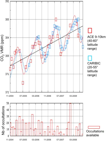
fit lines) in agreement with the mean annual growth rate ob-served at the surface for this time period (see, for example, http://www.esrl.noaa.gov/gmd/ccgg/trends/). CO 2 VMR (ppm) ACE 9-10km (40-60° latitude range) CARIBIC (20-55° latitude range) 11-2004 07-2005 03-2006 11-2006 07-2007 03-2008 11-2004 07-2005 03-2006 11-2006 07-2007 03-2008
Nb of occultations Occultations available
Fig. 5. Top: temporal evolution of CO2 concentration (y-axis
in ppm) in the upper troposphere (9–10 km). Blue boxes: ACE-FTS results for the 40◦N–60◦N latitude band; red boxes: CARIBIC measurements for the 20–55◦N latitude band. The blue and red lines result from a curve fit using a harmonic polynomial (two har-monics). The slope of the best fit line corresponds to the mean growth rate during this time period: 1.9 ppm.yr−1. Bottom: num-ber of ACE-FTS occultations used in the 9–10 km altitude range.
3.2 CO2below, around, and above the tropopause: from 8-9 km to 16-18 km
Figure 6 (top), which is similar to Fig. 5 but for the 50◦N–
60◦N latitude band and the 2004–2008 time period, displays
time series of ACE-retrieved monthly mean CO2
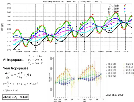
concen-trations for six atmospheric layers: 8–9 km, 9–10 km, 10– 12 km, 11–13 km, 12–14 km, and 16–18 km, spanning the upper troposphere to the lower stratosphere. Monthly mean retrieved concentrations are represented by crosses and the curves result from the harmonic polynomial fit (two harmon-ics for the first two layers, one harmonic for the remaining four) to the retrievals at different altitudes. Figure 6 (bot-tom), from Sawa et al. (2008), also displays CONTRAIL
CO2time series measurements above Eurasia in a similar
al-titude range from November 2005 to September 2007. Fig-ure 6 (top) can also be compared to results from SPURT (see Fig. 9 of Hoor et al. (2004) and Fig. 5 of Gurk et al. (2008))
Sawa et al., 2008 ) ( β α θ + ∂ ∂ = z T dz d 5 . 1 0 0≈ = T θ α =g/C ≈10−3K.m−1 p β θ Δ ≈ ΔZ(km) 0.1 θ Δ + = 0.1 ) (km Z0 Z K T K km Z 200 300 11 0 0 0 = = = θ At tropopause : Near tropopause :
Fig. 6. Top: Temporal evolution of CO2concentration retrieved from ACE-FTS measurements for six atmospheric layers from 8 to 18 km
(see color legend). Crosses show the retrievals (monthly mean) and the curves result from the harmonic polynomial fit (two harmonics for the first two layers, one for the remaining four) to the retrievals at different altitudes. Bottom: Temporal evolution of CO2concentration from
CONTRAIL measurements (Sawa et al., 2008) above Eurasia from November 2005 to September 2007. Each curve represents CO2time series observed at 10 K potential temperature bins from the local tropopause. An approximate relationship between θ (potential temperature) and altitude is given at the bottom left of the figure. Blue curves correspond to the lower stratosphere and orange curves to the higher troposphere.
particulary in term of seasonal variations. ACE-retrieved
CO2vertical profiles, SPURT and CONTRAIL in situ
mea-surements show key features of the CO2 distribution with
altitude. First, the amplitude of the CO2 tropospheric
sea-sonal cycle (detrended) decreases from 7–8 ppm below the tropopause at 9–10 km to 1–2 ppm at 10–12 km and the am-plitude increases again in the stratosphere at 16–18 km, in agreement with the observations but with an amplitude (2–3 ppm) somewhat too large for the highest layer. As pointed out by Hoor et al. (2004), the phase of the cycle remains tro-pospheric with a minimum in summer up to the lowermost stratosphere at 10–12 km, reflecting the strong coupling be-tween the lowermost stratosphere and the extra-tropical tro-posphere through trotro-posphere to stratosphere transport of air that entered the stratosphere at the tropical tropopause. The dampening of the amplitude of the seasonal cycle reflects the role of the extratropical tropopause as a barrier to transport (Hoor et al., 2004). Above, the phase maximum is shifted by up to three months towards summer as observed in-situ. Second, a negative vertical gradient is clearly seen in Fig. 6 in August which accurately reproduces the negative gradient
seen by SPURT and by CONTRAIL. This leads to a signifi-cant vertical gradient during winter and spring, and to a very weak gradient (sometimes positive) from 9 to 18 km in
sum-mer and fall. Third, at all altitudes the CO2concentration
ex-hibits a mean temporal trend of about 1.9 ppm.yr−1, again in
good agreement with the mean annual growth rate observed at the surface for this time period.
These comparisons show that the CO2concentrations
re-trieved from ACE-FTS are consistent with aircraft in situ measurements in the northern hemisphere mid-latitudes. In particular, the mean growth rate, the seasonal vertical gra-dient change and phase shift from the mid-troposphere to the lower stratosphere are well represented by ACE-retrieved
CO2 values. However the stratosphere seasonal cycle
am-plitude seems to be over-estimated. A possible explanation could come from the difference in the spatial coverage of the different data sets. Indeed, ACE-FTS results sum all latitudes
and longitudes in the 50◦N–60◦N band, whereas SPURT,
CARIBIC, and CONTRAIL data correspond to observations above Europe, Eurasia, and Asia, respectively.
4 Comparisons with air-transport model CO2profiles
Another way of assessing the quality of the ACE-retrieved
CO2 vertical profiles is to compare them with air transport
model simulations. For that purpose, two well known
mod-els have been used. First, we consider the Flexpart
La-grangian particulate dispersion model (Stohl et al., 2005) driven with meteorological input data (wind, temperature and humidity fields) from the European Centre for Medium
Range Weather Forecasts (ECMWF). CO2surface data from
the World Data Centre for Greenhouse Gases (WDCGG, http://gaw.kishou.go.jp/wdcgg) have been used to create a
source function for the lower most troposphere. CO2fields
from a six-year analysis have been monthly averaged for 10◦
latitude bands to make comparisons with profiles retrieved from ACE-FTS for the year 2006. The second model
con-sidered generates CO2model simulations from the
Carbon-Tracker (2009, http://carbontracker.noaa.gov) system (Peters et al., 2007). Carbon Tracker (CT) is based on the TM5 model, which is a global atmospheric chemistry-transport zoom model (Krol et al., 2005) optimized with highly
ac-curate CO2 measurements at the Earth’s surface from the
NOAA/ESRL network. Results have been averaged monthly
for the 50◦N–60◦N latitude band to make comparisons with
retrieved profiles from ACE-FTS for the years 2005 to 2008.
4.1 Monthly averaged CO2profiles
Figures 7 to 10 show model simulations (either CT alone or both CT and Flexpart) and ACE- retrieved profiles from 2005 to 2008, respectively, for the two months of May and July for
the 50◦N–60◦N latitude band. These two months are well
represented with respect to the number of occultations avail-able and show contrasting properties in terms of atmospheric transport. Both CT and Flexpart model standard deviations are around 1 ppm and ACE-retrieved profile standard devia-tion is about 4 ppm for the lowest altitude and about 2-3 ppm above. Figure 7 corresponds to 2005; ACE-retrieved profiles start around 400-500 hPa in the troposphere. Comparisons with CT profiles show a good overall agreement from 400 hPa to 70 hPa with a mean difference of less than 2 ppm. ACE values in May from 180 hPa to 70 hPa are smaller than the model values by about 2 ppm (however, less than 10 oc-cultations on average, are available). The large vertical gra-dient is seen by both products. In July, the ACE retrieved profile shows no vertical gradient contrary to CT that shows a ”peak” of about +3 ppm at about 180 hPa with respect to the 500 hPa value. Observations from SPURT show almost no gradient in July 2002 (Hoor et al., 2004) and observations from CONTRAIL show a gradient of about 4 ppm in July and of about 3 ppm in July 2007. Both ACE and CT however agree on a gradient that is much smaller in July than in May.
Figure 8 shows Flexpart, CT and ACE-retrieved CO2
pro-files in the 50◦N–60◦N latitude band for the months of May
and July 2006. A rather good agreement is found between
CO2VMR (ppm) CO2VMR (ppm)
Pressure (hPa) Pressure (hPa)
Fig. 7. CO2 concentration (x-axis in ppm) evolution with pres-sure (y-axis in hPa) for May (left) and July (right) for 2005 for the 50◦N–60◦N latitude band. ACE-retrieved profile is in red and CT profile is in blue. The thin red line indicates that less than 10 occul-tations were available. ACE CO2standard deviation at each altitude
(not shown in the picture) fluctuates around 3 ppm (±1 ppm).
these three sets of profiles. The difference is less than 2 ppm for most of the altitudes. In May, the Flexpart and CT profiles are very consistent in the troposphere whereas the difference reaches 2 ppm above the tropopause. The ACE-retrieved pro-file shows lower values (1.5 ppm) below 300 hPa and is closer to the Flexpart profile up to 100 hPa. At higher altitudes, a significant decrease in the ACE retrieved-profile is observed, not seen by the models. Between 100 and 200 hPa, ACE is between the two models. In July, the Flexpart profile is about 1 ppm higher than the CT profile at all the altitudes. ACE is closer to CT at lower altitudes and closer to Flexpart at higher altitudes. The vertical gradient is somewhat smaller for ACE than for the models.
Figure 9 shows results similar to Fig. 7 for the year 2007. The agreement between ACE-retrieved and CT simulated profiles is again good with a mean difference less than 1 ppm and gradients similar in May and slightly smaller for ACE in July. ACE-retrieved concentrations in the troposphere and higher in the stratosphere compare well with the model.
Figure 10 shows results similar to Fig. 7 for the year 2008. Here, the agreement is significantly worse with a mean
CO2VMR (ppm) CO2VMR (ppm)
Pressure (hPa) Pressure (hPa)
Fig. 8. CO2concentration (x-axis in ppm) evolution with pressure
(y-axis in hPa) for May (left) and July (right) of 2006 for the 50◦N– 60◦N latitude band. ACE-retrieved profile is in red, CT profile is in blue and Flexpart profile is in purple. ACE thin red line indicates that less than 10 occultations were available. ACE CO2standard
de-viation at each altitude (not shown in the picture) fluctuates around 3 ppm (±1 ppm).
difference of about 2 ppm especially above 250 hPa in May and 200 hPa in July. The difference is smaller in the tropo-sphere. The tropopause transition is smoother for ACE in May and steeper in July where a larger ACE gradient is seen. It must be pointed out that, for all years, the July peak value seen at about 200 hPa in CT profiles is also seen in ACE profiles but at significantly higher altitudes (except in 2006, where no peak value is seen in ACE profile).
These comparisons show that the CO2concentration
pro-files retrieved from ACE-FTS observations are quite consis-tent with model simulations in the northern hemisphere mid-latitudes for two particular months characterized by either a strong vertical gradient (May) or a weak (or no) gradient (July). The largest differences (3 ppm) are observed for the latter month.
4.2 Can a temporal shift of the model profiles improve the agreement with ACE-retrieved profiles?
Current problems with air-transport models have been briefly summarized in the Introduction. These model deficiencies can cause over or under estimation of tracer profiles, with the
CO2VMR (ppm) CO2VMR (ppm)
Pressure (hPa) Pressure (hPa)
Fig. 9. Same as Fig. 7 for 2007.
anomalies depending on the time of year and on the altitude (troposphere or stratosphere). As a consequence, a profile retrieved at a given month might more favourably be com-pared with a profile simulated by the model for the month just before or just after the month considered.
In this section we look for such temporal shifts between model profile simulations and ACE-retrieved profiles. We examine two years: 2006 which presents the best general agreement between ACE and CT, and 2008 which corre-sponds to the poorest agreement.
Figure 11 shows, for the 50◦N–60◦N latitude band,
ACE-retrieved profiles for May and July 2006 together with Flex-part and CT profiles for the months just after (June and Au-gust; top row) and for the months just before (April and June; bottom row). Although the original comparison showed gen-erally good agreement (see Fig. 8), a slight improvement is seen when comparing ACE in May to CT in June above 200 hPa and a more significant improvement in the agree-ment is seen when comparing ACE to both CT and Flexpart below 200 hPa (top-left). A slight degradation is observed when comparing ACE in May to both Flexpart and CT in April (bottom-left). A similar agreement is found when com-paring ACE in July to both models in August, except that ACE agrees better with Flexpart below 200 hPa than with CT (top-right); a strong degradation is observed when comparing ACE in July to both Flexpart and CT in June (bottom-right).
CO2VMR (ppm) CO2VMR (ppm)
Pressure (hPa) Pressure (hPa)
Fig. 10. Same as Fig. 7 for the year 2008.
CO2VMR (ppm) CO2VMR (ppm) CO2VMR (ppm) CO2VMR (ppm)
Pressure (hPa)
Pressure (hPa) Pressure (hPa)
Pressure (hPa)
Fig. 11. Flexpart (purple), CT (blue), and ACE (red) CO2profiles
for the 50◦N–60◦N latitude band in 2006. ACE profiles in May (left) and July (right) are compared to Flexpart and CT profiles of one month before (top), and of one month after (bottom). ACE thin red line indicates that less than 10 occultations were available.
Figure 12 shows, for the 50◦N–60◦N latitude band,
ACE-retrieved profiles for May and July 2008 together with Flex-part profiles for the months just after (June and August; top row) and for the months just before (April and June; bottom row). Compared to Fig. 10, the ACE profile in May agrees
CO
2VMR (ppm)
CO
2VMR (ppm)
CO
2VMR (ppm)
CO
2VMR (ppm)
Pressure (hPa)
Pressure (hPa) Pressure (hPa)
Pressure (hPa)
Fig. 12. CT (blue) and ACE (red) CO2profiles for the 50◦N–60◦N
latitude band in 2008. ACE profiles in May (left) and July (right) are compared to CT profiles of one month before (top), and of one month after (bottom). ACE thin red line indicates that less than 10 occultations were available.
better with the CT profile in June above 300 hPa but the fit is poorer below (top-left); the agreement is similar when com-paring ACE in May to CT in April (bottom-left). Compared to Fig. 10, the ACE profile in July agrees slightly better with the CT profile in August (top-right); the agreement is much poorer when comparing ACE in May to CT in June (bottom-right).
A provisional conclusion from this very limited exercise is that ACE-retrieved profiles agree better with model profiles for the month just after the ACE month considered. More comparisons are obviously required before concluding there is deficiency in the models or possible problems with the re-trievals.
A general agreement between model-simulated and
ACE-retrieved profiles for the 50◦N–60◦N latitude band in May
and July is evident from this comparison. However, differ-ences are observed notably above and around the tropopause region. We also observe that comparing the ACE profile in May to model profiles in April improves the fit (mean and standard deviation) for all years considered here. The improvement is less significant in July. A strong degrada-tion generally occurs when comparing ACE profiles in July
circulation strength might be over estimated during the north-ern hemisphere spring. Obviously, this does not exclude er-rors in the retrieval method and many more comparisons of retrievals vs. models are required before a convincing con-clusion can be drawn.
5 Conclusions
In this paper we have presented, for the first time in the 5–
25 km altitude range, five years of monthly mean CO2
ver-tical profiles from the ACE-FTS limb-viewing space-borne instrument (Bernath et al., 2005). After having briefly re-viewed the inversion approach described in detail in Fal2009, results obtained for the 2004–2008 time period and for the
40◦N–60◦N and 50◦N–60◦N latitude bands have been
com-pared with in situ aircraft measurements from the CON-TRAIL (Sawa et al., 2008), CARIBIC (Schuck et al., 2009), and SPURT (Gurk et al., 2008) in situ aircraft measurements,
as well as with two air transport model CO2 profile
sim-ulations: Flexpart (Stohl et al., 2005) and Carbon Tracker (Peters et al., 2007). These comparisons have shown that
the CO2concentrations retrieved from ACE-FTS are
consis-tent with aircraft measurements in the northern hemisphere mid-latitudes. In particular, the mean growth rate, the sea-sonal vertical gradient change and phase shift from the mid-troposphere to the lower stratosphere are well represented by
ACE-retrieved CO2 values. However the stratosphere
sea-sonal cycle amplitude (16–18 km) seems somewhat over es-timated. A possible explanation could come from the dif-ference in the spatial coverage of the different data sets. In-deed, ACE-FTS results cover all latitudes and longitudes of
the 40◦N–60◦N and 50◦N–60◦N bands, whereas SPURT,
CARIBIC, and CONTRAIL data correspond to observation above Europe, Eurasia, and Asia, respectively. Comparisons for two particular months, May (characterized by a strong vertical gradient) and July (characterized by a weak – or no –
gradient) have shown that the CO2concentration profiles
re-trieved from ACE-FTS observations are quite consistent with model simulations in the northern hemisphere mid-latitudes. However, differences are observed notably above and around the tropopause region. Current deficiencies in air-transport models may cause over or under estimates of tracer profiles, and these anomalies depend on the time of the year and on the altitude (troposphere or stratosphere). For this reason, we looked for temporal shifts between model profile simula-tions and ACE-retrieved profiles and observed that compar-ing ACE profiles in May to model profiles in April improves the fit for all the years considered here. The improvement is less significant in July. A strong degradation generally oc-curs when comparing ACE profiles in July to model profiles in June. This suggests that the model circulation strength is over estimated during the northern hemisphere spring. Ob-viously, this does not exclude errors in the retrieval method and more comparisons are required before a firm conclusion
can be drawn. Future developments include: (i) the
improve-ment of the modelling of the N2continuum absorption; (ii)
the processing of the years 2009 and 2010; (iii) the analysis of other latitude bands and specific geographic regions with a better space-time resolution.
This new ACE-FTS CO2profile database provides
infor-mation on air transport and data for assimilation into models. Coupled with column measurements from a nadir viewing instrument, it may also be expected that occultation measure-ments will bring useful constraints to the surface carbon flux determination.
Appendix A
ACE retrieved monthly mean profiles from 2004 to 2008
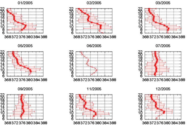
We present in this appendix (Fig. A1 to A3) monthly
aver-aged ACE-retrieved CO2profiles for the nine months
avail-able in the 50◦N–60◦N latitude band.
Acknowledgements. The ACE mission is supported primarily
by the Canadian Space Agency (CSA) and some support was provided by the Natural Environment Research Council (NERC) of the UK. We gratefully acknowledge J. M. Hartmann for providing us with the N2 continuum CIA laboratory measure-ments and for fruitful discussions which led to their integration in our RTM. CarbonTracker 2009 results were provided by NOAA ESRL, Boulder, Colorado, USA through the website at http://carbontracker.noaa.gov. We especially wish to thank A. Ja-cobson and W. Peters for their help. Warm thanks are also extended to N. A. Scott and to V. Capelle for their important contributions to the development of the Radiative Transfer Model used here and to B. Legras for his help in the handling of the Flexpart model. We are happy to thank the two anonymous reviewers for their constructive and helpful comments.
Edited by: P. O. Wennberg
Fig. A1. Monthly mean CO2concentration (x-axis in ppm) evolution with altitude (y-axis in km) for nine months of 2005 for the 50◦N–
60◦N latitude band. Horizontal bars correspond to the standard deviation of retrieved CO2profiles for each altitude. ACE thin red line
indicates that less than 10 occultations were available; in that case, standard deviation is not estimated.
Fig. A3. Same as Fig. A1 for 2007.
References
Anderson, B., Gregory, G., Collins, J. J., Sachse, G., Conway, T., and Whiting, G.: Airborne observations of spatial and temporal variability of tropospheric carbon dioxide, J. Geophys. Res., 101, 1985–1997, 1996.
Andrew, A. E., Boering, K. A., Daube, B. C.,Wofsy, S. C., Loewen-stein, M., Jost, H., Podolske, J. R.,Webster, C. R., Herman, R. L., Scott, D. C., Flesch, G. J., Moyer, E. J., Elkins, J. W., Dutton, G. S., Hurst, D. F., Moore, F. L., Ray, E. A., Romashkin, P. A., and Strahan, S. E.: Mean ages of stratospheric air derived from in situ observations of CO2, CH4, and N2O, J. Geophys. Res.,
106, 32295–32314, 2001.
Baker, D. F., Law, R. M., Gurney, K. R., Rayner, P., Peylin, P., Denning, A. S., Bousquet, P., Bruhwiler, L., Chen, Y. H., Ciais, P., Fung, I. Y., Heimann, M., John, J., Maki, T., Maksyutov, S., Masarie, K., Prather, M., Pak, B., Taguchi, S., and Zhu, Z.: TransCom3 inversion intercomparison: Interannual variabil-ity of regional CO2fluxes, Global Biogeochem. Cy., 1988–2003,
doi:10.1029/2004GB002439, 2006.
Beagley, S. R., Boone, C. D., Fomichev V. I., Jin, J. J., Semeniuk, K., McConnell, J. C., Bernath, P. F.: First multi-year occultation observations of CO2in the MLT by ACE satellite: observations and analysis using the extended CMAM, Atmos. Chem. Phys.,
10, 1133–1153, 2010,
http://www.atmos-chem-phys.net/10/1133/2010/.
Bernath, P. F.: Atmospheric Chemistry Experiment (ACE): Analyt-ical Chemistry from Orbit, Trends Anal. Chem., 25, 647–654, 2006.
Bernath, P. F., McElroy, C. T., Abrams, M. C., Boone, C. D., Butler, M., Camy-Peyret, C., Carleer, M., Clerbaux, C., Coheur, P.-F., Colin, R., DeCola, P., DeMaziere, M., Drummond, J. R., Dufour, D., Evans, W. F. J., Fast, H., Fussen, D., Gilbert, K., Jennings, D. E., Llewellyn, E. J., Lowe, R. P., Mahieu, E., Mc-Connel, J. C., McHugh, M., Mcleod, S. D., Michaud, R., Midwinter, C., Nas-sar, R., Nichitiu, F., Nowland, C., Rinsland, C. P., Rochon, Y. J., Rowlands, N., Semeniuxk, K., Simon, P., Skelton, R., Sloan, J. J., Soucy, M. A., Strong, K., Tremblay, P., Turnbull, D., Walker, K. A., Walkty, I., Wardle, D. A., Wehrle, V., Zander, R., and Zou, T.: Atmospheric Chemistry Experiment (ACE): Misson overview, Geophys. Res. Lett., 32, L15S01, doi:10.1029/2005GLO22386, 2005.
B¨onisch, H., Hoor, P., Gurk, C., Feng, W., Chipperfield, M., En-gel, A., and Bregman, B.: Model evaluation of CO2and SF6in
the extratropical UT/LS region, J. Geophys. Res., 113, D06101, doi:10.1029/2007JD008829, 2008.
Boone, C. D., Nassar, R.,Walker, K. A., Rochon, Y., Mcleod, S. D., Rinsland, C. P., and Bernath, P. F.: Retrievals for the
Atmo-spheric Chemistry Experiment Fourier-Transform Spectrome-trer, App. Opt., 44, 7218–7231, 2005.
Brenninkmeijer, C. A. M., Crutzen, P. J., Fischer, H., Gsten, H., Hans, W., Heinrich, G., Heintzenberg, J., Hermann, M., Im-melmann, T., Kersting, D., Maiss, M., Nolle, M., Pitscheider, A., Pohlkamp, H., Scharffe, D., Specht, K., and Wiedensohler, A.: CARIBIC: Civil Aircraft for Global Measurement of Trace Gases and Aerosols in the Tropopause Region, J. Atmos. Ocean. Tech., 16, 1373–1383, 1999.
Brenninkmeijer, C. A. M., Crutzen, P., Boumard, F., Dauer, T., Dix, B., Ebinghaus, R., Filippi, D., Fischer, H., Franke, H., Frie?, U., Heintzenberg, J., Helleis, F., Hermann, M., Kock, H. H., Koep-pel, C., Lelieveld, J., Leuenberger, M., Martinsson, B. G., Miem-czyk, S., Moret, H. P., Nguyen, H. N., Nyfeler, P., Oram, D., O’Sullivan, D., Penkett, S., Platt, U., Pupek, M., Ramonet, M., Randa, B., Reichelt, M., Rhee, T. S., Rohwer, J., Rosenfeld, K., Scharffe, D., Schlager, H., Schumann, U., Slemr, F., Sprung, D., Stock, P., Thaler, R., Valentino, F., van Velthoven, P., Waibel, A., Wandel, A., Waschitschek, K., Wiedensohler, A., Xueref-Remy, I., Zahn, A., Zech, U. and Ziereis, H.: Civil aircraft for the reg-ular investigation of the atmosphere based on an instrumented container: The new CARIBIC system, Atmos. Chem. Phys., 7, 4943–4976, doi:10.5194/acp-7-4943-2007, 2007.
Buchwitz, M., de Beek, R., Noel, S., Burrowsandi, J. P., Bovens-mann, H., Bremer, H., Bergamaschi, P., Krner, S., and HeiBovens-mann, M.: Carbon monoxide, methane and carbon dioxide columns re-trieved from SCIAMACHY by WFM-DOAS: year 2003 initial data set., Atmos. Chem. Phys., 5, 3313–3329, doi:10.5194/acp-5-3313-2005, 2005.
Ch´edin, A., Serrar, S., Armante, R., Scott, N. A., and Hollingsworth, A.: Signatures of annual and seasonal variations of CO2and other greenhouse gases from comparisons between
NOAA/TOVS observations and model simulations, J. Climate, 15, 95–116, 2002.
Ch´edin, A., Scott, N. A., Crevoisier, C., and Armante, R.: First global measurement of mid-tropospheric CO2from NOAA
po-lar satellites: the tropical zone, J. Geophys. Res., 108, 4581, doi:10.1029/2003JD003439, 2003a.
Ch´edin, A., Saunders, R., Hollingsworth, A., Scott, N. A., Ma-tricardi, M., Etcheto, J., Clerbaux, C., Armante, R., and Crevoisier, C.: The feasibility of monitoring CO2 from
high-resolution infrared sounders, J. Geophys. Res., 108, 4064, doi:10.1029/2001JD001443, 2003b.
Crevoisier, C., Heilliette, S., Ch´edin, A., Serrar, S., Armante, R., and Scott, N. A.: Midtropospheric CO2concentration retrieval
from AIRS observations in the tropics, Geophys. Res. Lett., 31, L17106, doi:10.1029/2004GL020141, 2004.
Crevoisier, C. Ch´edin, A., Scott, N. A., Matsueda, H., Machida, T., and Armante, R.: First year of upper tropospheric integrated con-tent of CO2from IASI hyperspectral infrared observations,
At-mos. Chem. Phys., 9, 4797–4810, doi:10.5194/acp-9-4797-2009, 2009.
Dudhia, A., Jay, V. L., and Rodgers, C. D.: Microwindow selection for high-spectral-resolution sounders, App. Opt., 41, 3665–3673, 2002.
Engel, A., B¨onish, H., Brunner, D., Fischer, H., Franke, H., Gunter, G., Gurk, C., Hegglin, M., Hoor, P., K¨onigstedt, R., Krebach, M., Maser, R., Parchatka, U., Peter, T., Schell, D., Schiller, C., Schmidt, U., Spelten, N., Szabo, T., Weers, U., Wernli, H.,
Wetter, T., and Wirth, V.: Highly resolved observations of trace gases in the lowermost stratosphere from the Spurt project: an overview, Atmos. Chem. Phys., 6, 283–301, doi:10.5194/acp-6-283-2006, 2006.
Engelen, R. J. and McNally, A. P.: Estimating atmospheric CO2from advanced infrared satellite radiances within an
oper-ational four-dimensional varioper-ational (4D-Var) data assimilation system: Results and validation, J. Geophys. Res., 110, D18305, doi:10.1029/2005JD005982, 2005.
Foucher, P. Y., Ch´edin, A., Dufour, G., Capelle, V., Boone, C. D., and Bernath, P.: Technical Note: Feasibility of CO2
profile retrieval from limb viewing solar occultation made by the ACE-FTS instrument, Atmos. Chem. Phys., 9, 2873–2890, doi:10.5194/acp-9-2873-2009, 2009a.
Foucher, P. Y., D´etermination de profils verticaux de concentration en CO2 atmosph´erique partir d’observations spatiales.
Appli-cation aux donn´es en occultation solaire de l’instrument ACE-FTS sur SCISAT 1. PhD thesis, University Pierre et Marie Curie, Paris, 2009b.
Gelb, A.: Applied Optimal Estimation, M.I.T. Press, 180–229, 1974.
Gurney, K. R., Law, R. M., Denning, A. S., Rayner, P. J., Baker, D., Bousquet, P., Bruhwiler, L., Chen, Y. H., Ciais, P., Fan, S., Fung, I. Y., Gloor, M., Heimann, M., Higuchi, K., John, J., Maki, T., Maksyutov, S., Masarie, K., Peylin, P., Prather, M., Pak, B. C., Randerson, J., Sarmiento, J., Taguchi, S., Takahashi, T., and Yuen, C. W.: Towards robust regional estimates of CO2sources
and sinks using atmospheric transport models, Nature, 415, 626– 630, 2002.
Gurk, Ch., Fischer, H., Hoor, P., Lawrence, M. G., Lelieveld, J., and Wernli, H.: Airborne in-situ measurements of vertical, seasonal and latitudinal distributions of carbon dioxide over Europe, At-mos. Chem. Phys., 8, 6395–6403, doi:10.5194/acp-8-6395-2008, 2008.
Hegglin, M. I., Boone, C. D., Manney, G. L., T.G.Shephered, Walker, K. A., Bernath, P. F., Daffer, W. H., Hoor, P., and Schiller, C.: Validation of ACE-FTS satellite data in the upper troposphere/lower stratosphere (UTLS) using non-coincident measurements, Atmos. Chem. Phys., 8, 1483–1499, doi:10.5194/acp-8-1483-2008, 2008.
Hoor, P., Gurk, C., Brunner, D., Hegglin, M. I., Wernli, H., and Fischer, H.: Seasonality and extent of extratropical TST derived from in-situ CO measurements during SPURT, Atmos. Chem. Phys., 4, 1427–1442, doi:10.5194/acp-4-1427-2004, 2004. Horowitz, L. W., Walters, S., Mauzerall, D. L., Emmons, L. K.,
Rasch, P. J., Granier, C., Tie, X., Lamarque, J. F., Schultz, M. G., Tyndall, G. S., Orlando, J. J., and Brasseu, G. P.: A global simulation of tropospheric ozone and related tracers: Description and evaluation of MOZART, version 2, J. Geophys. Res., 108, 4784, doi:10.1029/2002JD002853, 2003.
Jacquinet-Husson, N., Scott, N. A., Ch´edin, A., Cr´epeau, L., Ar-mante, R., Capelle, V., Orphal, J., Coustenis, A., Boonne, C., Poulet-Crovisier, N., Barbe, A., Birk, M., Brown, L. R., Camy-Peyret, C., Claveau, C., Chance, K., Christidis, N., Clerbaux, C., Coheur, P. F., Dana, V., Daumont, L., Backer-Barilly, M. R. D., Lonardo, G. D., Flaud, J. M., Goldman, A., Hamdouni, A., Hess, M., Hurley, M. D., Jacquemart, D., Kleiner, I., Kpke, P., Mandin, J. Y., Massie, S., Mikhailenko, S., Nemtchinov, V., Nikitin, A., Newnham, D., Perrin, A., Perevalov, V., Pinnock, S.,
Rgalia-Jarlot, L., Rinsland, C., Rublev, A., Schreier, F., Schult, L., Smithu, K. M., Tashkun, S. A., Teffo, J. L., Toth, R. A., Tyuterev, V. G., Auwera, J. V., Varanasi, P., and Wagner, G.: The GEISA spectroscopic database: Current and future archive for Earth and planetary atmosphere studies, J. Quant. Spectrosc. Radiat. Transfer, 100, 1043–1059, 2008.
Koner, P. K. and Drummond, J. R.: Atmospheric trace gases pro-file retrievals using the nonlinear regularized total least square method, J. Quant. Spectrosc. Radiat. Transfer, 109, 2045–2059, doi:10.1016/j.jqsrt.2008.02.014, 2008.
Krol, M., Houweling, S., Bregman, B., van den Broek, M., Segers, A., van Velthoven, P., Peters, W., Dentener, F., and Bergamaschi, P.: The two-way nested global chemistry-transport zoom model TM5: algorithm and applications, Atmos. Chem. Phys., 5, 417– 432, doi:10.5194/acp-5-417-2005, 2005.
Kulawik, S. S., Jones, D. B. A., Nassar, R., Irion, F. W., Worden, J. R., Bowman, K. W., Machida, T., Matsueda, H., Sawa, Y., Biraud, S. C., Fischer, M. L. and Jacobson, A. R.: Character-ization of Tropospheric Emission Spectrometer (TES) CO2for carbon cycle science, Atmos. Chem. Phys., 10(12), 5601–5623, doi:10.5194/acp-10-5601-2010, 2010.
Kuze, A., Suto, H., Nakajima, M., and Hamazaki, T.: Initial On-board Performance of TANSO-FTS on GOSAT, in Fourier Trans-form Spectroscopy, OSA Technical Digest, Optical Society of America, 2009.
Lafferty, W. J., Solodov, A. M., Weber, A., Olson, W. B., and Hart-mann, J.-M.: Infrared collision-induced absorption by N2near
4.3 µm for atmospheric applications: measurements and empiri-cal modeling, App. Opt., 35, 5911–5917, 1996.
Levenberg, K. :A Method for the Solution of Certain Non-Linear Problems in Least Squares. The Quarterly of Applied Mathemat-ics 2, 164–168, 1944.
Machida, T., Matsueda, H., Sawa, Y., Nakagawa, Y., Hirotani K., Kondo, N., Goto, K., Nakazawa, T., Ishikawa, K., and Ogawa T.: Worldwide measurements of atmospheric CO2and other trace gas species using commercial airlines, J. Atmos. Oceanic Tech-nol., 25, 1744–1754, 2008.
Matsueda, H., Taguchi, S., Inoue, H. Y., and Ishii, M.: A large impact of tropical biomass burning on CO and CO2in the upper
troposphere, Science China Press, 45, 116–125, 2002.
Matsueda, H., T. Machida, Y. Sawa, Y. Nakagawa, K. Hirotani, H. Ikeda, N. Kondo, and K.Goto: Evaluation of atmospheric CO2 measurements from new air sampling of JAL airliner observa-tions, Papers in Meteorology and Geophysics, 59, 1–17, 2008. Marquardt, D.: An Algorithm for Least-Squares Estimation of
Nonlinear Parameters. SIAM J. Appl. Math., 11, 431-441, doi:10.1137/0111030, 1963.
Nakazawa, T., Miyashita, K., Aoki, S., and Tanaka, M.: Tempo-ral and spatial variations of upper troposphere and lower strato-spheric carbon dioxide, Tellus, 43B, 106–117, 1991.
Niro, F., Boulet, C., Hartmann, J.-M.: Spectra calculations in cen-tral and wing regions of CO2IR bands between 10 and 20 µm.
I- Model and laboratory measurements, J. Quant. Spectrosc. Ra-diat. Transfer, 88, 483–498, 2004.
Olsen, S. C. and Randerson, J. T.: Differences between sur-face and column atmospheric CO2 and implications for
carbon cycle research, J. Geophys. Res., 109, D02301, doi:10.1029/2003JD003968, 2004.
Pak, B. C. and Prather, M. J.: CO2source inversions using satellite
observations of the upper troposphere, Geophys. Res. Lett., 28, 4571–4574, 2001.
Park, J. H.: Atmospheric CO2monitoring from space, App. Opt., 36, 2701–2712, 1997.
Patra, P. K., Maksyutov, S., Sasano, Y., Nakajima, H., Inoue, G., and Nakazawa, T.: An evaluation of CO2 observations with
Solar Occultation FTS for Inclined-Orbit Satellite sensor for surface source inversion, J. Geophys. Res., 108(D24), 4759, doi:10.1029/2003JD003661, 2003.
Peters, W., Jacobson, A. R., Sweeney, C., Andrews, A. E., Conway, T. J., Masarie, K., Miller, J. B., Bruhwiler, L. M. P., P´etron, G., Hirsch, A. I., Worthy, D. E. J., van der Werf, G. R., Randerson, J. T., Wennberg, P. O., Krol, M. C., and Tans, P. P.: An atmospheric perspective on North American carbon dioxide exchange: Car-bonTracker, Proc. Natl. Acad. Sci. USA,, 27 November 2007, 104(48), 18925–18930, 2007.
Phillips, D. L.:A Technique for the Numerical Solution of Certain Integral Equations of the First Kind, J. Assoc. Comput. Mach., 9, 84–97, 1962.
Plumb, R.: A “tropical pipe” model of stratospheric transport, J. Geophys. Res., 301, 3957–3972, 1996.
Plumb, R. and Ko, M.: Interrelationships between mixing ratios of long-lived stratosphere constituents, J. Geophys. Res., 97, 10145–10156, 1992.
Rinsland, C. P., Chiou, L. S., Boone, C., and P. Bernath P.: Car-bon dioxide retrievals from Atmospheric Chemistry Experiment solar occultation measurements, J. Geophys. Res., 115, D03105, doi:10.1029/2009JD012081, 2010.
Rodgers, C. D.: Inverse methods for atmospheric sounding. Theory and practice, World scientific, Singapore, 2000.
Sawa, Y. , Machida, T. and Matsueda, H.: Seasonal variations of CO2 near the tropopause observed by commercial aircraft, J.
Geophys. Res., 113, D23301, doi:10.1029/2008JD010568, 2008. Schuck, T. J., Brenninkmeijer, C. A. M., Slemr, F., Xueref-Remy, I., and Zahn, A.: Greenhouse gas analysis of air samples collected onboard the CARIBIC passenger aircraft, Atmos. Meas. Tech., 2, 449–464, doi:10.5194/amt-2-449-2009, 2009.
Scott, N. A.: A direct method of computation of transmission func-tion of an inhomogeneous gaseous medium : descripfunc-tion of the method and influence of various factor, J. Quant. Spectrosc. Ra-diat. Transfer, 14, 691–707, 1974.
Scott, N. A. and Ch´edin, A.: A fast line-by-line method for atmo-spheric absorption computation: The Automatized Atmoatmo-spheric Absorption Atlas, J.Appl.Meteorol., 20, 801–812, 1981. Shia, R. L., Liang, M. C., Miller, C. E., and Yung, Y.
L.: CO2 in the upper troposphere: Influence of
strato-spheretroposphere exchange, Geophys. Res. Lett., 33, L1481, doi:10.1029/2006GL026141, 2006.
Steck, T.: Methods for determining regularization for atmospheric retrieval problems, App. Opt., 41, 1788–1797, 2002.
Stohl, A., C. Forster, A. Frank, P. Seibert, and G. Wotawa, Techni-cal Note: The Lagrangian particle dispersion model Flexpart ver-sion 6.2, Atmos. Chem. Phys. 5, 2461–2474, doi:10.5194/acp-5-2461-2005, 2005.
Tikhonov, A. N.: On the regularization of ill-posed problems. Dokl. Akad. Nauk SSSR, 153 49–52; MR, 28, 5577; Soviet Math. Dokl., 4 (1963), 1624–1627, 1963
Twomey, S.: On the Numerical Solution of Fredholm Integral Equa-tions of the First Kind by the Inversion of the Linear System
Pro-duced by Quadrature, J. Assoc. Comp. Mach., 10, 97–101, 1963. von Clarmann, T. and Echle, G.: Selection of optimized microwin-dows for atmospheric spectroscopy, App. Opt., 37, 7661–7669, 1998.
von Clarmann, T., Glatthor, N., Grabowski, U., Hopfner, M., Kell-mann, S., Kiefer, M., Linden, A., Tsidu, G. M., Milz, M., Steck, T., Stiller, G. P., Wang, D. Y., Fischer, H., Funke, B., and Gil-L´opez-Puerta, S.: Retrieval of temperature and tangent altitude pointing from limb emission spectra recorded from space by the Michelson Interferometer for Passive Atmospheric Sounding (MIPAS), J. Geophys. Res., 108, 4736–4750, 2003.