Mining Complex Hydrobiological Data with Galois Lattices

HAL Id: hal-00531756

https://hal.archives-ouvertes.fr/hal-00531756

Submitted on 3 Nov 2010

HAL is a multi-disciplinary open access archive for the deposit and dissemination of sci-entific research documents, whether they are pub-lished or not. The documents may come from

L’archive ouverte pluridisciplinaire HAL, est destinée au dépôt et à la diffusion de documents scientifiques de niveau recherche, publiés ou non, émanant des établissements d’enseignement et de

Lattices

Aurélie Bertaux, Florence Le Ber, Agnès Braud, Michèle Trémolières

To cite this version:

Aurélie Bertaux, Florence Le Ber, Agnès Braud, Michèle Trémolières. Mining Complex Hydrobiologi-cal Data with Galois Lattices. International Journal of Computing and Information Sciences (IJCIS), APCEP - Canada, 2010, 7 (2), pp.63–77. �hal-00531756�

Mining Complex Hydrobiological Data with

Galois Lattices

Aurélie Bertaux

1,2

_{, Florence Le Ber}

1,3

_{, Agnès Braud}

2

_{, and}

Michèle Trémolières

1

(1) _{LHyGeS UMR 7517 – ENGEES - UDS - CNRS}

1 quai Koch, BP 61039, F 67070 Strasbourg cedex, FRANCE

{aurelie.bertaux, florence.leber}@engees.u-strasbg.fr michele.tremolieres@unistra.fr

(2)_{LSIIT UMR 7005}

Bd Sébastien Brant, BP 10413, F 67412 Illkirch cedex, FRANCE

agnes.braud@urs.u-strasbg.fr

(3)_{LORIA UMR 7503}

BP 35, F 54506 Vandœuvre-lès-Nancy cedex, FRANCE

Abstract: We used Galois lattices for mining hydrobiological data about macrophytes, i.e. macroscopic plants living in water bodies. These plants are characterized by several biological traits, that are divided into several modalities. Our aim was to cluster the plants according to their common traits and modalities and to find out the relations between the traits. Galois lattices are efficient methods for such an aim, but apply to binary data. In this article, we detail a few of the approaches we used to turn complex hydrobiological data into binary data and compare the first results obtained thanks to Galois lattices.

Keywords: Galois Lattices, Formal Concept Analysis, Multi-valued Data, Conceptual Scales, Multiple Correspondence Analysis.

1. Introduction

Water quality is a major problem in Europe, underlined by the recent European Water Framework Directive. A main issue is to evaluate the quality of the whole ecosystem, with respect to the pressures it undergoes (chemical pollutions, buildings, lack of water ...). In France, for example, running waters are qualified with physico-chemical parameters or with five biological indices based on floristic (diatoms and macrophytes) and faunistic (invertebrates, oligochaetes and fishes) species. The advantage of bio-indication tools over approaches based only on physico-chemical parameters is that they keep track of ephemeral pressures like pollutions; nevertheless, their results are difficult to compare since they are based on compartmental expertise. Thus, both physico-chemical approaches and biological indices seem not to be sufficient and new tools are required for evaluating the quality of the whole ecosystem (Bazerques, 2004). Furthermore a comparison of the tools and approaches is necessary to get a coherent monitoring of water bodies in Europe.

The work presented in this paper is part of a wider project which aims at comparing the answers of the bio-indication tools with respect to the various pressures undergone by water bodies (Grac et al., 2006). One particular issue is that biological indices rely on faunistic or floristic species which do not live

everywhere, preventing a wide comparison of indices. A promising approach to avoid this drawback is to determine ecological traits, shared by different species of different areas, that could be used to characterize the functioning of aquatic systems and thus, water quality, rather than the species themselves (Lafont et

al., 2001; Lafont, 2001). Currently, these ecological traits still have to be defined

for most compartments of aquatic systems. According to this statement, our work aims at helping hydrobiologists to find out relevant ecological traits of macrophytes ‒or hydrophytes‒ based on the description of their biological (and physical) characteristics and on the description of their habitat.

Firstly we focused on biological characteristics of macrophytes. More precisely, we used data collected from the literature and adapted for the macrophytes living in the Alsace plain (Staerck, 2005; Willby et al., 2000). We proposed to explore these data with the help of Galois lattices or formal concept analysis (Barbut & Montjardet, 1970; Davey & Priestley, 1990; Ganter & Wille, 1999). The aim was to search for concepts, i.e. sets of biological characteristics owned by a group of species, which could be interpreted with respect to the functioning of the ecosystem and thus lead to ecological traits. We have chosen to use Galois lattices because they are useful tools for knowledge extraction (Hereth et al., 2000; Napoli, 2006) and they allow to organize knowledge in a hierarchical way which is quite natural for hydrobiologists. Nevertheless, since the dataset was not a binary table, usual algorithms could not be used straight away, and it was necessary to explore various approaches that gave different results, as we show in this paper.

The paper is organized as follows. The first part is the current introduction, the second part presents the dataset in concern and the data mining approaches used in the hydrobiological domain, while the third part gives some definitions about formal concept analysis. The fourth and fifth parts explain the methods we used to convert the dataset into a suitable format. The sixth part sets out the results we obtained and a discussion, while the last part offers some conclusions and perspectives of our work.

2. Hydrobiological data

Indications about the quality of water bodies are given by several parameters, belonging to two main categories, the physico-chemical and the biological parameters. They give different insights, as the former allow to detect the pollution only when it happens or just after, and the latter reflect the integration of the pollution by the living organisms and thus show it later and longer. Some countries in Europe have proposed and adopted various systems to evaluate water quality, based either on physico-chemical or biological parameters. For the moment none of them is completely satisfactory and since the systems adopted are different it is not possible to get a coherent view of the state of water across Europe. Hydrobiologists from the LHyGeS lab work at defining a system that would overcome the problems mentioned by collecting and analyzing several datasets (Grac et al., 2006). We propose to design adequate data mining tools for that purpose.

2.1 Methods for analyzing hydrobiological data

As done in the biological and ecological domains (James & McCulloch, 1990), hydrobiologists mainly use multivariate analysis methods for analyzing the data they collect, but various data mining approaches have also been experimented (Džeroski, 2001). Works often aim at designing models allowing a better understanding of the relations between the diversity of a small community of living organisms and the biological, environmental or physico-chemical characteristics of the water body. For example, Goethals (2005) dealt with the problem of predicting macro invertebrate communities present in rivers using artificial neural networks (ANNs) and classification trees.

ANNs have been widely studied in ecological modeling as the ecological systems are highly nonlinear. However, the fact that they give good prediction results may be weakened by the black-box character of the approach which makes it difficult to understand (Blockeel et al., 1999). This is a severe drawback as far as validation by the expert is concerned and thus it prevents from tuning the system according to the remarks the expert may formulate on the results.

Other approaches are available such as classification and regression trees which give results in a readable format. In (Džeroski et al., 1997), the authors worked on data from British and Slovenian rivers. They dealt with the task of predicting a class of abundance for species using the CN2 system for rule induction. In (Džeroski & Grbović, 2001), regression trees were used to investigate further the relations between physico-chemical properties of water and the diversity of living organisms. These works show how symbolic methods facilitate the discussion with experts, and how it can help to tune the system.

All the works described above use machine learning methods, relying on labeled data. As far as we know, unsupervised classification methods, such as formal concept analysis, have not been used for exploring hydrobiological data, nor similar data. Actually, the search for functional traits or groups has been done with statistical approaches, like hierarchical clustering or multiple correspondence analysis (Hérault & Honnay, 2007; Lafont et al., 2001). These approaches rely on complex metrics and reveal only the main properties of a dataset. On the contrary, Galois lattices allow to explore the whole dataset in a rather simple and understandable form and can be used to complete multivariate methods (Duquenne, 1999; Hereth et al., 2000).

2.2 A dataset about the biological characteristics of macrophytes

The data we deal with are about macrophytes, or hydrophytes, i.e. macroscopic species living in water bodies. They were collected from the literature, and they represent a general knowledge about the biological characteristics of the macrophytes living in the Alsace plain. They were originally built from several observations and with the help of statistical methods as explained in (Willby et

al., 2000).

In the dataset, each species is described by a set of biological traits, i.e. physical and physiological characteristics, like the potential size, the reproduction period or the growing form. For each trait there are several qualitative modalities. For example, the 'potential size' trait has four modalities: “under 0.08 meter”,

“between 0.08 and 0.3 meter”, “between 0.3 and 1 meter”, “between 1 and 5 meters”. The 'reproduction period' trait owns four modalities (couples of months from March to October)...

Each modality is associated to a value between 0 and 3 that represents the

affinity of the species towards the modality ‒built on statistical observations

(Willby et al., 2000). The 0 value means that there is no individual having this modality, 1 means that a few individuals of the species have it, 2 a bit more, and 3 many. For example, the 'potential size' of Berula erecta (BERE) is given by the 4-set (1, 2, 3, 0) while it is (0, 1, 2, 2) for Callitriche obtusangula (CALO), which means, in particular, that you will never find a water celery (Berula erecta) greater than 1 meter and no blunt-fruited water starwort (Callitriche

obtusangula) smaller than 0,08 meter (see Table 1).

The triple (trait, modality, affinity) allows to describe the biological characteristics of macrophytes in a qualitative and rather complex way. For example, the data we deal with represents 21 species for which we have all the information, and they are described by 10 traits and 37 modalities.

3. Galois lattices for complex datasets

We give here some useful definitions about Galois lattices. In the second part the approaches dealing with Galois lattices and complex data will be described.

3.1 Definitions

Galois lattices or formal concept lattices (Barbut & Montjardet, 1970; Davey &

Priestley, 1990; Ganter & Wille, 1999) work on binary data to perform clustering of objects and attributes (clusters are called concepts) and to extract

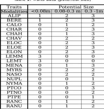
Table 1: Traits data (potential size)

Traits Potential Size Modalities <0.08m 0.08-0.3 m 0.3 -1m ALIP 1 2 3 BERE 1 2 3 CALO 0 1 2 CHAR 0 2 3 CHAH 0 1 3 CHAV 0 2 2 ELOC 0 2 3 ELOE 0 2 3 ELON 0 2 3 LEMM 3 0 0 LEMT 3 0 0 MENA 0 1 3 MYRS 0 2 2 NASO 0 2 2 NUPL 0 0 1 NYMA 0 1 2 PTCO 0 0 3 PTNO 0 0 2 PTPE 0 0 1 RANC 0 1 2 RANU 0 1 2

implications sets between attributes (Duquenne, 1987; Duquenne & Guigues, 1986).

A context is a triple K:=(G,M,I) where G and M are two sets and I a binary relation on GM. The elements of G are called objects, the elements of M are called attributes, and gIm means that the object g owns the attribute m according to I. If A is a subset of G,

A' = {m M | for all g A: ∈ ∈ gIm}. If B is a subset of M,

B' = {g G | for all m B: gIm}∈ ∈

This couple of mappings (A -> A'; B -> B'), is said to be a Galois connection between the G and M sets. From this connection, we get a set of concepts (A, B), such that B' = A and A' = B, that are organized within a concept lattice of K. A is a set of objects, called the extent, and B is a set of attributes, called the intent. In the following, the infimum (or meet) of a finite subset of concepts C is denoted by ∧C and the supremum (or join) of C is denoted by ∨C. A concept c of the Galois lattice is join-irreducible if c = ∨C for a finite subset C implies that

c ∈ C. Similarly, c is meet-irreducible if c = ∧C implies that c ∈ C.

A many-valued context K is defined in (Ganter & Wille, 1999) as a quadruple (G,

M, V, I), where G is a set of objects, M is a set of many-valued attributes, V is a

set of attribute values, and I is a ternary relation, I ⊆ GMV such that: (g, m, v) ∈ I and (g, m, w) ∈ I always implies w=v.

The notation (g, m, v) ∈ I (or m(g) = v) means that the m attribute has the v value for the g object.

3.2 Methods for dealing with complex data

Complex data were processed into the Galois lattice theory through the definition of conceptual scales, or through specific approaches such as fuzzy lattices.

Conceptual scales (Ganter & Kuznetsov, 2001;, 26] have been defined in order to deal with increasing amounts of data and with many-valued contexts, and are used to group related attributes. In (Ganter & Wille, 1997), a conceptual scale is defined for a many-valued attribute m as a one-valued context which has the attribute values of m among its objects. A scale can be associated to each many-valued attribute m, and m is replaced by the set of its scale attributes. Each value of m is substituted by the corresponding row of the scale. This approach introduces straight away a hierarchy between attributes, and may be useful to save time during the calculation of the lattice.

Many-valued contexts can also be processed within the theory of fuzzy lattices (Bělohlávek, 1999), which relies on the idea that the I relation between the objects and the attributes of a context is not only true or false, but takes values into [0; 1]. More precisely, let C = (G, M, I) be a formal fuzzy context, with G a set of objects, M a set of attributes, and I a fuzzy relation. Let D ⊆ G be a set of objects and P a fuzzy set of attributes defined in M. The Galois connection is defined by the operators f and h as:

− f (D) is a fuzzy set of attributes m _{where  is a degree of truth equal to the}

minimum of the degree of truth of m towards all objects of d ∈ D.

− (P) is the set of all objects owning each mh  _{attribute ∈ P with a degree of}

truth greater than .

A general approach for dealing with complex attributes, like intervals or histograms, has been defined in (Polaillon, 1998). Since the classical approach was too restrictive for such data, it was suggested to build and compare two lattices: the union lattice, where the concept intent contains all the properties of the individuals belonging to the extent, and the intersection lattice, where the concept intent contains the properties belonging to all the individuals of the extent. Furthermore, specific Galois connections were defined, depending on the attribute formats, e.g. for histogram data, m = Ө(g) = [Ө1_{, Ө}2_{, Ө}3 _{...], the Galois} connections could be defined as follows (the other notations used are those of the definition of the classical Galois lattice).

− Union lattice:

A' = {[maxg A∈ Ө1, maxg A∈ Ө2, maxg A∈ Ө3 ...]} B' = {g | for all m B, ∈ Ө(g) ≤ m}

− Intersection lattice:

A' = {[ming A∈ Ө1, ming A∈ Ө2, ming A∈ Ө3 ...]} B' = {g | for all m B, ∈ Ө(g) ≥ m}

3.3 Our approach

The dataset about biological traits of macrophytes is a many-valued context with special form (G, M, V, W, I), where G is a set of species, M is a set of many-valued traits, V is a set of modalities, W is a set of affinities, and I is a 4-ary relation. We call it a fuzzy many-valued context. The specificities of these data can be taken into account through the various methods described above. In this paper we focus on the transformation of the context with various scales. In a preliminary step of our work (section 4), this context was converted in a straightforward way into a complete disjunctive table, which is a binary table corresponding to nominal scaling. In a second step (section 5), we defined a special scale in order to preserve the distribution of affinities over the trait modalities.

4. A complete disjunctive table

The result of the nominal scaling of the biological trait context is shown in Table 2. The names of the new attributes follow a 'Lxy' model: the letter 'L' denotes a trait ('S' for potential Size, 'R' for potential of Regeneration...), 'x' is a number which shows the index of a modality and 'y' is the affinity value. For example, S21 means “few individuals (affinity 1) having a potential size (S)

between 0.08 and 0.3 m (2nd _{modality)”. For clarity purposes, these new} attributes are called “properties” in the following.

This binary table can be used to build a Galois lattice, but is also a traditional data format for multivariate analysis, which is classically used in hydrobiology. Thus the results obtained with the Galois lattice (section 4.1) are compared to those of multi correspondence analysis (section 4.2).

4. 1 The Galois lattice

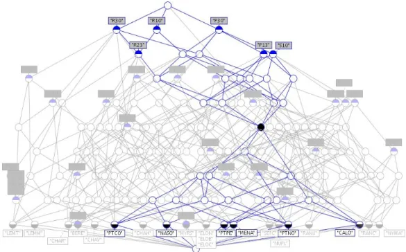
Figure 1 shows the Galois lattice based on a restriction of the disjunctive table to three traits: potential size S, perennation P and potential of regeneration R. The whole lattice contains 1849 concepts, i.e. sets of macrophytes sharing the same modalities of the same traits with the same affinity. We used the ConExp tool (Yevtushenko et al., 2000-2006) both to build and to analyze the lattice. ConExp allows to edit a context, to draw the associated lattice, to calculate the Duquenne-Guigues-Basis (Duquenne & Guigues, 1986) for implications between properties, and to give the association rules that are true in this context.

We looked for groups of species having the same trait modalities, living in the same water environment, that could serve as indicators for the quality of this environment. Hydrobiologists found it more relevant to work with concepts owning between 4 and 5 properties, because few properties represent too generalized a group, while too many show too specialized a situation in terms of the environment behavior.

For example, the concept in black on Figure 1, namely ({R10, R23, R30, P13, P30, S10}, {PTNO, PTCO, CALO, MENA, NASO, PTPE}), means that the 6 (among 21) following species, Potamogeton nodosus, Potamogeton coloratus,

Callitriche obtusangula, Mentha aquatica, Nasturtium officinale, and Potamogeton pectinatus, share the same following trait modalities:

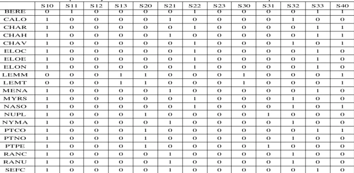
Table 2. The complete disjunctive table of traits data restricted to the potential size trait

S10 S11 S12 S13 S20 S21 S22 S23 S30 S31 S32 S33 S40 BERE 0 1 0 0 0 0 1 0 0 0 0 1 1 CALO 1 0 0 0 0 1 0 0 0 0 1 0 0 CHAR 1 0 0 0 0 0 1 0 0 0 0 1 1 CHAH 1 0 0 0 0 1 0 0 0 0 0 1 1 CHAV 1 0 0 0 0 0 1 0 0 0 1 0 1 ELOC 1 0 0 0 0 0 1 0 0 0 0 1 0 ELOE 1 0 0 0 0 0 1 0 0 0 0 1 0 ELON 1 0 0 0 0 0 1 0 0 0 0 1 0 LEMM 0 0 0 1 1 0 0 0 1 0 0 0 1 LEMT 0 0 0 1 1 0 0 0 1 0 0 0 1 MENA 1 0 0 0 0 1 0 0 0 0 0 1 0 MYRS 1 0 0 0 0 0 1 0 0 0 1 0 0 NASO 1 0 0 0 0 0 1 0 0 0 1 0 1 NUPL 1 0 0 0 1 0 0 0 0 1 0 0 0 NYMA 1 0 0 0 0 1 0 0 0 0 1 0 0 PTCO 1 0 0 0 1 0 0 0 0 0 0 1 1 PTNO 1 0 0 0 1 0 0 0 0 0 1 0 0 PTPE 1 0 0 0 1 0 0 0 0 1 0 0 0 RANC 1 0 0 0 0 1 0 0 0 0 1 0 0 RANU 1 0 0 0 0 1 0 0 0 0 1 0 0 SEFC 1 0 0 0 0 1 0 0 0 0 0 1 0

• period of reproduction (R): (R1) "March-April" = 0, (R2) "May-June" = 3,

(R3) "July-August" = 0

• perennation (P): (P1) "perennial underground organs" = 3, (P3)

"annual" = 0

• potential size (S): (P1) "smaller than 0.08m" = 0.

This set of traits represents both physiological and physical aspects. Actually, the main common point between the 6 species is that they live in running as well as standing waters and can be submerged. It cannot be directly linked to a specific functioning of the ecosystem but if more traits are taken into account, better results can be obtained, as we will see further.

For a better interpretation of this context, we can use the Duquenne-Guigues implications (Duquenne & Guigues, 1986). Considering the whole lattice (148 Lxy properties, 1849 concepts), we can extract 582 implications. An AB implication, deduced from the lattice, concerns attributes A and B of a same concept. The confidence of an implication is always 100% and the support is the number of objects in the extension of this concept, i.e. the number of species having both attributes A and B. For our data: 17 implications have a support between 19 and 14 (more than 2/3 of the species), 383 between 5 and 1 (less than 1/4 of the species). Finally there are only 37 implications supported by at least half of the species, which we assume to be representative of the dataset.

Looking further at the representative implications, it can be seen that their components mainly represent a lack of a trait modality rather than its presence. For example, let us examine the following implication (1): C30 D30 F10 => M50 (support=16). This implication can be read as follows: species which do not have a rigid stem (C30), nor a low potential of dispersion (D30), nor a weak flexibility (F10), do not have a big volume (M50). This negative implication reveals in contrast the characteristics of strict hydrophytes that have a medium volume, a medium or high flexibility, and a submerged flexible stem.

The implications with lower support may reveal specific relationship between trait modalities. For example (2) C30 D23 => F20 (support=9), means that a species which does not have a rigid stem (C30) and mainly an intermediate level of dispersion (D23) does not have a medium flexibility (F20). Relying on the interpretation of implication (1), this second implication can be transformed within (3) D23 => (F3 ≠ 0), highlighting the link between an intermediate level dispersion and a high flexibility for some strict hydrophytes.

Furthermore, these implications have been used to validate the dataset. Indeed the implications and their supports were examined in order to detect incorrect, useless or redundant data.

4.2 A multivariate method

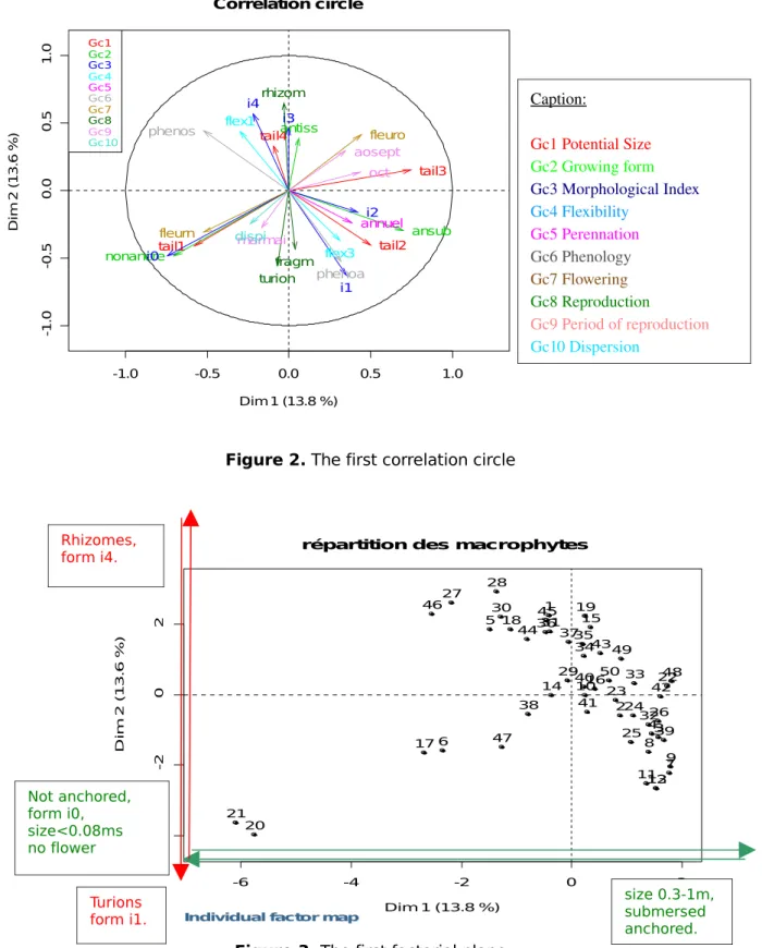
Building a Galois lattice from the binary table is interesting since it allows a comparison with statistical methods used by hydrobiologists. Indeed the dataset (actually a larger dataset (Pinçon, 2008)), presented in section 2, has been analyzed with a multivariate method, the MCA (Multiple Correspondence Analysis). This method relies on mathematical projections in order to visualize the main features of a dataset. For instance, Figure 2 shows the first correlation circle, where the main contributions are due to two groups of trait modalities:

• Factor 1: potential size, first (<0.08m) and third (0.3-1m) modalities;

growing form "not anchored" and "submersed, anchored" modalities; morphological index, first modality (i0); flowering, "no" modality; phenology, "seasonal" modality.

• Factor 2: reproduction, "by rhizome" and "by turions" (i.e. underground

buds) modalities; morphological index, second and fifth modalities; phenology, "annual" modality.

According to this result, the species represented in the first projection plan (Figure 3) can be interpreted as follows:

• Species at the top-right of the plan: Berula erecta (2), Potamogeton

coloratus (33) and Zanichellia palustris (50) are characterized by their

growing form (submersed, anchored) and their potential size (0.3-1m).

• Species at the top of the plan: e.g. Nuphar lutea (27), Nymphea alba (28),

Juncus articualtus (19), Phalaris arundinaceae (30) and 3 species of

Potamots (34,35,37) have a similar morphological index (i4) and a similar vegetative reproduction (rhizomes or stolons).

• Species at the bottom-left of the plan: Lemna minor (20) and L. trisulca

flower. Furthermore, they have turions and their morphological index is low (i1). -1.0 -0.5 0.0 0.5 1.0 -1 .0 -0 .5 0 .0 0 .5 1 .0 Correlation circle Dim 1 (13.8 %) D im 2 ( 1 3 .6 % ) Gc1 Gc2 Gc3 Gc4 Gc5 Gc6 Gc7 Gc8 Gc9 Gc10 tail1 tail2 tail3 tail4 nonancre antiss ansub i0 i1 i2 i3 i4 flex1 flex3 annuel phenoa phenos _fleuro fleurn rhizom turion fragm marmai aosept oct dispi

Figure 2. The first correlation circle

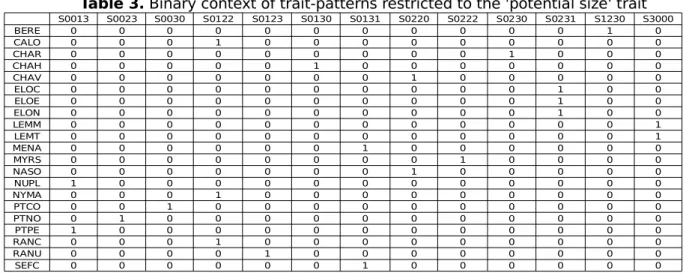
Figure 3. The first factorial plane

Caption: Gc1 Potential Size   Gc2 Growing form  Gc3 Morphological Index  Gc4 Flexibility   Gc5 Perennation Gc6 Phenology Gc7 Flowering Gc8 Reproduction Gc9 Period of reproduction Gc10 Dispersion -6 -4 -2 0 2 -4 -2 0 2

répartition des macrophytes

Dim 1 (13.8 %) D im 2 ( 1 3 .6 % )

Individual factor map

1 2 3 4 5 6 7 8 9 10 11₁₂₁₃ 14 15 16 17 18 19 20 21 22 23 24 25 26 27 28 29 30 31 32 33 34 35 36 37 38 39 40 41 42 43 44 45 46 47 48 49 50 Turions form i1. size 0.3-1m, submersed anchored. Not anchored, form i0, size<0.08ms no flower Rhizomes, form i4.

The results of MCA are quite easy to read and give some interesting characteristics of the dataset. The main problem is that each plan represents only a small part of the whole information. In Figure 3, the first plan represents 13.6 + 13.8 = 27.4% of the total inertia. So, several projection plans should be examined and the synthesis is not always easy. Furthermore, the clustering of species and trait modalities is quite "rough" and does not make what is really common or different among the species explicit. The use of Galois lattices can help to overcome these difficulties even if it involves new problems. For example, we can search for the species clusters resulting from the MCA within the concepts of the Galois lattice, and thus better analyze the structure of these clusters.

For example, looking at the bottom-right of the plan (Figure 3), it seems that the group of species, Chara fragilis (7), Chara vulgaris (9), Elodea canadensis (11), and Elodea ernstae (12), can be characterized by a potential size between 0.3 and 1 meter and a submersed, anchored growing form. The Galois lattice confirms that these macrophytes share these attributes with other species:

Berula erecta (2) and Elodea nuttallii (13) which belong to the same concept.

5. Pattern approaches

This section focuses on another type of conversion of the initial table, that keeps the information about the repartition of species affinities among the modalities. Actually, the conversion of the original data within a complete disjunctive table entails three main problems. Firstly, a lattice with 1849 concepts is not easily readable. Secondly, the number of implications is high, and most of them are negative implications giving little information. Thirdly, this conversion breaks a single distribution of affinities into several properties wrt the different modalities of a trait, whereas this is meaningful for hydrobiologists. To overcome this problem, we have tested another approach which is detailed below.

Let us examine an example of what we would like to represent. For instance, consider the BERE plant (Berula erecta), whose affinities towards the "potential size" trait are (1, 2, 3, 0), according to the four modalities of this trait. This pattern (1, 2, 3, 0) is interesting for the hydrobiologists, because it shows the continuity of the size distribution of Berula erecta. Furthermore, having two species with (almost) the same distribution is more meaningful than having two species with the same affinity for one or two modalities. Thus, we have tried another conversion of the initial dataset, which we call Pattern[0,3], and then a variant that represents the distributions of affinities with percentages.

5.1 Pattern[0,3]

Our aim is to represent the distribution of the affinities of a species according to the various modalities of a trait as a unique property, called a trait-pattern. This pattern is composed as follows: first comes a letter that refers to the trait (like 'S' for potential Size) and then nt numbers that refer to the affinity values of the nt modalities. For example S0122 means “the potential size of members of this species is never of the first modality (<0.08 m), sometimes of the second modality (between 0.08 and 0.3 m), often of the third and fourth modalities

(between 0.3 and 1 m and between 1 and 5 m)”. According to this choice, the

dataset about the biological traits of macrophytes can be written as a binary context (G, M, I), where G is a set of species, M is a set of trait-patterns, and I is a binary relation.

Table 3. Binary context of trait-patterns restricted to the 'potential size' trait

The corresponding binary table, manually built, is shown on Table 3 for the potential size. Looking at this table, one can see that very few patterns are common to more than two individuals. The lattice built from the whole dataset has 95 concepts spread over 6 levels (excepting top and bottom) and is shown on Figure 4. We can see most of the patterns belong to only one individual.

Furthermore, from the whole lattice, 234 implications were extracted whose support is under 5, such as F0030 D030 => G30. This means that only 5 species (for the best result) support these implications. This is due to the pattern model which is very accurate so that only a few macrophytes match each of them.

To get around this problem we need to increase the number of shared properties. For hydrobiologists, the spreading of the modalities over the traits expresses an important piece of information, that can also be represented by a percentage. Actually, an affinity value can be considered as a part of species individuals owning a specific modality. This allows to have fewer patterns with probably more representative ones.

5.2 Pattern[0,3]%

Let us consider the potential size pattern (1, 2, 3, 0) of Berula erecta. It means that this species has very few individuals owning the first modality, some owning the second, a lot owning the third and none the fourth. This can be understood as a distribution of probabilities such as (0.17, 0.33, 0.50, 0), meaning that 17% of the individuals of this species have the first modality, 33% the second modality, 50% the third and 0% the fourth. With this approach, the patterns (0, 2, 2, 0) and (0, 1, 1, 0) represent the same distribution (0, 0.5 , 0.5, 0) that will be shared by more species.

S0013 S0023 S0030 S0122 S0123 S0130 S0131 S0220 S0222 S0230 S0231 S1230 S3000 BERE 0 0 0 0 0 0 0 0 0 0 0 1 0 CALO 0 0 0 1 0 0 0 0 0 0 0 0 0 CHAR 0 0 0 0 0 0 0 0 0 1 0 0 0 CHAH 0 0 0 0 0 1 0 0 0 0 0 0 0 CHAV 0 0 0 0 0 0 0 1 0 0 0 0 0 ELOC 0 0 0 0 0 0 0 0 0 0 1 0 0 ELOE 0 0 0 0 0 0 0 0 0 0 1 0 0 ELON 0 0 0 0 0 0 0 0 0 0 1 0 0 LEMM 0 0 0 0 0 0 0 0 0 0 0 0 1 LEMT 0 0 0 0 0 0 0 0 0 0 0 0 1 MENA 0 0 0 0 0 0 1 0 0 0 0 0 0 MYRS 0 0 0 0 0 0 0 0 1 0 0 0 0 NASO 0 0 0 0 0 0 0 1 0 0 0 0 0 NUPL 1 0 0 0 0 0 0 0 0 0 0 0 0 NYMA 0 0 0 1 0 0 0 0 0 0 0 0 0 PTCO 0 0 1 0 0 0 0 0 0 0 0 0 0 PTNO 0 1 0 0 0 0 0 0 0 0 0 0 0 PTPE 1 0 0 0 0 0 0 0 0 0 0 0 0 RANC 0 0 0 1 0 0 0 0 0 0 0 0 0 RANU 0 0 0 0 1 0 0 0 0 0 0 0 0 SEFC 0 0 0 0 0 0 1 0 0 0 0 0 0

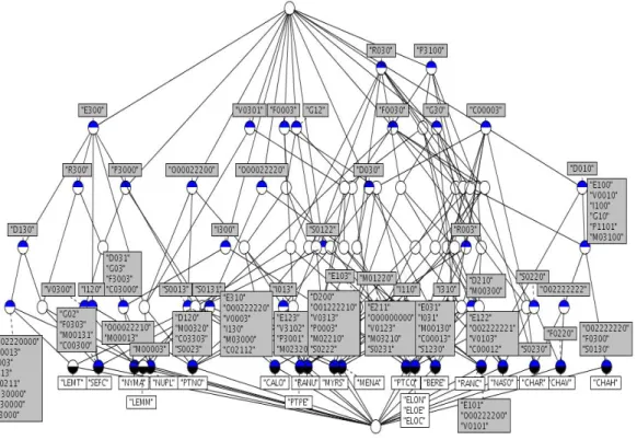
Figure 4. The Galois lattice built from the pattern table (all traits).

The new trait-pattern model, which we call Pattern[0,3]%, has the same format as Pattern[0,3]: a letter for the trait followed by the percentage of each modality, e.g. S0122 is equivalent to S-0-20-40-40. The resulting lattice contains 105 concepts. It also has 221 implications such as:

F-0-0-100-0 D-0-100-0 => G-100-0 (support=6).

This rule is a more general version of the F0030 D030 => G30 rule obtained with the Pattern[0,3] format, and which had a support equal to 5.

This representation of the data is more suitable for hydrobiologists because it takes the spreading of the species over the modalities into account, and seems to be more interesting for our purpose, since it gives less attributes than the

Pattern[0,3] representation. The lattices obtained with those two representations are compared in the next section.

6. Results and discussion

In a first step we compare formally the lattices built on the two pattern datasets. In a second step we describe the approach used for interpreting the lattices according to hydrobiological knowledge.

6.1 Comparison of the pattern-lattices

Two lattices were built based on the pattern datasets. The first one (Pattern[0,3]) respects the whole information. The second one (Pattern [0,3](%)) focuses on the distribution of affinities towards the modalities of a trait and does not take the information about abundance into account. It would be interesting to compare the two lattices for evaluating the ratio gain/loss of the two approaches. Basically, this comparison can be done on the basis of numerical characteristics of the lattices, e.g. number of concepts, objects, attributes, implications, etc. To summarize these characteristics, we can also use the set of irreducible concepts, since each V lattice can be represented by the reduced context (J(V), M(V), ≤) where J(V) is the set of all ∨-irreducible elements of V and M(V) the set of all ∧-irreducible elements of V (Ganter & Wille, 1999).

The numerical results presented in Table 4 show that the two lattices are based on 21 objects and 10 traits. Attributes are the trait-patterns (modality-affinity) and we can logically see that the conversion into percentage decreases the number of attributes. The number of concepts, the number of implications and the number of edges of the lattices are very similar for the two lattices. If we look at the ratio between the concepts, we obtain 95/105=0.9; between the attributes we have 110/103=1.1; and between the implications: 234/221 =1.1. All these ratios are close to 1. Furthermore, the numbers of join-irreducible and meet-irreducible concepts and the heights of the two lattices are exactly the same.

Thus the structures of the two lattices are very similar. Nevertheless this is not enough to conclude about the equivalence of the lattices. So we will take a closer look at the join and meet-irreducibles as done in (Napoli & Le Ber, 2007). As the two lattices are built on the same set of species, we can immediately see that the join-irreducible elements are exactly the same in the two lattices (each species is represented separately in one join-irreducible element except ELOC, ELOE, ELON which have exactly the same attributes), and so we will focus on the meet-irreducible concepts. Therefore, we first match the concepts with respect to their intent, then compare the objects of their extent (see Table 5). The 30 meet-irreducible concepts of the Pattern[0,3]-lattice are separated into three groups. The first group contains 25 concepts, which are associated to

Table 4. Numerical comparison of the structures of the pattern lattices

Pattern [0,3] Pattern [0,3] (%) number of objects 21 21 nb of traits 10 10 nb of attributes 110 103 nb of concepts 95 105 nb of implications 234 221 join irreducible 19 19 meet irreducible 30 30 nb of edges 220 249 height 7 7

identical concepts of the Pattern[0,3]%-lattice. The second group includes 4 concepts which are associated to quite similar concepts of the Pattern[0,3]%-lattice, as shown in Table 5. Actually the intents are identical, but the extents in

Pattern[0,3]% contain (as expected) more species than in Pattern[0,3], e.g. the

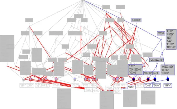
two concepts {E300}{LEMT, SEFC, NYMA, NUPL, LEMM, PTNO, MYRS}, and {E-100-0-0}{LEMT, SEFC, NYMA, NUPL, LEMM, PTNO, MYRS, CHAR, CHAH, CHAV} are identified. The last group contains only one concept (line 5 in Table 5) which cannot be associated to the last concept of the Pattern[0,3]%-lattice: neither the intents nor the extents do match. Figure 5 illustrates the meet-irreducible concept {D010,C0003} from Pattern[0,3]-lattice (line 5 of Table 5), which inherits from the concept {C0003}; while Figure 6 highlights the meet-irreducible {F0-50-50-0, G100-0, R0-100-0} from Pattern[0,3]%-lattice which inherits from {G100-0} and {R0-100-0}.

Table 5. Differences between meet-irreducible concepts of Pattern[0,3] and Pattern[0,3]% contexts

extent for Pattern[0,3] intent for Pattern[0,3] intent for Pattern[0,3](%) more extent for Pattern[0,3]% 1 {CALO, MYRS, MENA, ELON, {G30} {G 100 0 } {+CHAR, CHAH, CHAV}

ELOC, ELOE, BERE, NASO},

2 {LEMT, SEFC, NYMA, NUPL, {E300} {E 100 0 0} {+CHAR, CHAH, CHAV}

LEMM, PTNO, MYRS},

3 {CALO, PTPE, ELON, ELOC, ELOE, BERE}, {D030} {D-0-100-0} {+CHAR, CHAH, CHAV, RANC, RANU} 4 {NYMA, NUPL, ELON, ELOC, ELOE}, {I300} {I100-0-0} {+CHAH, CHAV} 5 {RANC, CHAR, CHAV, CHAH}, {D010, C00003} {F0-50-50-0, G100-0, R0-100-0} {CHAV MENA}

From these statements, we can conclude that most attributes of Pattern[0,3] and

Pattern[0,3]% are identical (i.e. the corresponding columns of the binary tables

are identical). Only five columns of the reduced contexts (J(V), M(V), ≤) are different, with more objects associated to the Pattern[0,3]% meet-irreducibles vs. the Pattern[0,3] meet-irreducibles (except for the pair {D010, C00003} / {F0-50-50-0, G100-0, R0-100-0}).

Finally the Pattern[0,3]%-lattice appears to be more efficient towards knowledge extraction requests, with little information lost. From this conclusion and because it better fits the hydrobiologists expectations in terms of representing the spreading of the species among the modalities, we will use the

Pattern[0,3]% format for future work.

6.2 An analysis from a hydrobiological point of view

As said in the previous section, this preliminary analysis relies on the

Pattern[0,3]%-lattice. From this lattice, we have extracted the "middle"

concepts, whose extent contains 4 to 7 species. This interval has been chosen with respect to the total number of species and the balance between the number of species and the number of associated attributes.

Figure 5. Meet-irreducible concept {D010,C0003}

Each set of species is then related to the features of the places where the species live (their habitat). For example, the four species RANT, PTCR, MYRS, RANC, have the same characteristics (Growth form 100, Flexibility 0-0-0-100, Dispersion 100-0-0) which means that they are submerged species, flexible, and with a high dispersion. Furthermore, they live in eutrophic water bodies. Besides, the six species UTRV, PTLU, CERD, PHAA, PTNA, PTCR, have the Flexibility 0-0-0-100, Perennation 100-0-0, Phenology 0-100 attributes, and live in calm water bodies.

Based on the relations between the species and their biological traits given by the lattice, and the relations between species and the ecological features of their habitat, we were able to link these features to biological traits in order to determine ecological traits for the macrophytes, i.e. traits describing the way they belong to their environment. For example, the trait "tolerance to change in

humidity" describes how species bear to be sometimes out of water. The trait

"tolerance to organic matter" describes how species endure the carbonaceous material produced by living beings or due to man (anthropic) inputs. Four ecological traits have been defined. We are currently working at describing the modalities of these traits and the affinities of the species.

Ecological traits are an abstraction of the species, allowing to compare the water quality from different areas where the species are not the same but share the same behavior within their environment. Ecological traits can thus be used in the design of a general tool for the evaluation of water quality, as we aim to do.

7. Conclusion and future work

We are working on the design of a new evaluation system of the quality of water bodies. An important problem wrt this purpose is to be able to compare the quality of water bodies in different regions and to build a coherent evaluation system over Europe. Analyzing biological traits and determining ecological traits of species is a promising approach as traits allow to evaluate water quality in a more general way than the species themselves.

In this paper, we have focused on the analysis of the biological traits of macrophytes, that are vegetable species living in water. We have proposed to use Galois lattices in order to extract groups of biological traits shared by groups of species on the one hand, and to analyze the implications between biological traits on the other hand. We have pointed out the fact that the data about biological traits are represented as triples (trait, modality, affinity) which make them too complex to directly build a lattice from them. We have thus studied two conversions from those data into binary ones: the first one scatters the information within a full disjunctive table while the second one concatenates the couple (trait, modalities) within one single histogram-like attribute whose values are patterns which represent the distributions of species over affinities

wrt the modalities of biological traits.

The results obtained from the first conversion were compared to those of MCA, a multivariate method used in the ecological domain. Furthermore, the analysis of the concepts and implications gave some interesting results for hydrobiologists, but the lattice built on the whole dataset (21 species, 148

attributes) appeared to be too large, and gave scattered information. Conversely, the second conversion gave a small set of concepts and implications with very low supports. Nevertheless, we were able to extract some interesting concepts, i.e. groups of macrophytes and their biological traits, which were associated to the functional characteristics of their usual habitat and thus led to the definition of the ecological traits of macrophytes.

To sum up, we can say the Galois lattice is a new approach in the hydrobiological domain and it appears to be well suited. To go further, we propose to investigate the benefits of using lattices with a more complex structure, as those defined in (Bělohlávek, 1999; Latiri Cherif et al., 2003; Polaillon, 1998; Stumme, 1999). We will keep the idea of repartition embedded in the pattern approach, but we will allow a partial matching between the patterns. For example, when looking at the two S1230 and S0122 trait-patterns (potential size of BERE and CALO), one can see that the median part contains values in the two patterns (23/12) or that the ranks are moved forward in the CALO pattern with respect to the BERE pattern. To take this information into account, we can use fuzzy lattices, or union/intersection lattices as proposed in (Polaillon, 1998). According to this approach, BERE and CALO could form a union-concept where the intent contains S1232, and an intersection-concept where the intent contains S0120.

Such lattices allow to get more general concepts, grouping species with similar

vs. identical attributes. They should overcome the problems of the two

approaches already used: the information on the distributions will be kept, but it will be generalized so that it will produce more useful concepts. Following this line, we plan to develop a tool to deal with such complex data, to build various lattices according to specific attribute matchings, and to extract the interesting concepts.

Acknowledgments

The authors thank the Agence de l'Eau Rhin Meuse and the Région Alsace for supporting this work.

References

M. Barbut, B. Monjardet, Ordre et classification – Algèbre et combinatoire, Hachette, Paris, France, 1970.

M.-F. Bazerques, “Directive-cadre sur l’eau : le bon état écologique des eaux douces de surface, sa définition, son évaluation”, Communication au Ministère de l’Écologie et

du Développement Durable, Paris, 2004.

R. Bělohlávek, “Fuzzy Galois Connections”, Math. Logic Quaterly, vol. 45, 1999, pp. 497-504.

H. Blockeel, S. Džeroski, J. Grbović, “Simultaneous prediction of multiple chemical parameters of river water quality with TILDE”, In Proc. Third European Conference

on Principles of Data Mining and Knowledge Discovery, 1999, pp. 15-18.

B. Davey, H. Priestley, Introduction to Lattices and Order, Cambridge University Press, Cambridge, UK, 1990.

V. Duquenne, “Contextual implications between attributes and some representational properties for finite lattices”, In Beiträge zur Begriffsanalyse, B.I.

Wissenschaftsverlag, Mannheim, 1987, pp. 213-239.

V. Duquenne, Latticial structures in data analysis, Theoretical Computer Science, vol. 217, 1999, pp. 407-436.

V. Duquenne, J.-L. Guigues, “Famille minimale d’implications informatives résultant d’un tableau de données binaires”, Math. et Sci. Hum., vol. 24(95), 1986, pp. 5–18.

S. Džeroski, “Applications of symbolic machine learning to ecological modelling”,

Ecological Modelling, vol. 146, 2001, pp. 263-273.

S. Džeroski, J. Grbović, “Relating biodiversity of river communities to physical and chemical water properties”, In Proceedings Sustainability in the information society

(Fifteenth International Symposium on Informatics for Environmental Protection),

Marburg, Metropolis, Part. 1, 2001, pp. 367-372.

S. Džeroski, J. Grbović, W. J. Walley, B. Kompare, “Using machine learning techniques in the construction of models. Part II: Rule induction”, Ecological Modelling, vol. 95, 1997, pp. 95-111.

B. Ganter, S. Kuznetsov, “Pattern Structures and Their Projections”, In Proceedings of

the 9th International Conference on Conceptual Structures (ICCS 2001), Springer,

LNCS, vol. 2120, 2001, pp. 129-142.

B. Ganter, R. Wille, “Applied Lattice Theory: Formal Concept Analysis”, General Lattice

Theory, G. Grätzer editor, Birkhäuser, 1997.

B. Ganter, R. Wille, Formal Concept Analysis: Mathematical foundations, Springer, 1999. P. Goethals, “Data driven development of predictive ecological models for benthic

macroinvertebrates in rivers”, PhD Thesis, Universiteit Gent. Faculteit Bio-ingenieurswetenschappen, 2005.

C. Grac, A. Herrmann, F. Le Ber, M. Trémolières, A. Braud, A. Handja, N. Lachiche, “Mining a database on Alsatian rivers”, In Proceedings of the 7th International

Conference on Hydroinformatics, HIC 2006, Nice, France, vol. III, 2006, pp.

2263-2270.

B. Hérault, O. Honnay, “Using life-history traits to achieve a functional classification of habitats”, Applied Vegetation Science, vol. 10, 2007, pp. 73-80.

J. Hereth, G. Stumme, R. Wille, U. Wille, “Conceptual Knowledge Discovery and Data Analysis”, In Proceedings of the 8th International Conference on Conceptual

Structures (ICCS'00), Darmstadt, LNAI 1867, 2000, pp. 421-437.

F.C. James, C.E. McCulloch, “Multivariate Analysis in Ecology and Systematics: Panacea or Pandora's Box?”, Annual Review of Ecology and Systematics, vol. 21, 1990, pp. 129-166.

M. Lafont, P. Breil, P. Namour, J.-C. Camus, F. Malard, P. Le Pimpec, “Concept d'ambiance écologique dans les systèmes aquatiques continentaux (AESYS)”, In Actes du

séminaire "État écologique des milieux aquatiques continentaux", Cemagref

Éditions, 2001, pp. 136-153.

M. Lafont, A conceptual approach to the biomonitoring of freshwater: the Ecological Ambience System, J. Limnol., vol. 60 (Suppl. 1), 2001, pp. 17-24.

C. Latiri Cherif, J.-P. Chevallett, S. Elloumi, A. Jaoua, “Une extension de la connexion de Galois floue pour la recherche d'information”, Information Interaction Intelligence, vol. 3(2), 2003, pp. 73-116.

A. Napoli, “A smooth introduction to symbolic methods in knowledge discovery”, In

Categorization in Cognitive Science, H. Cohen and C. Lefebvre editors, Elsevier,

Amsterdam, 2006.

A. Napoli, F. Le Ber, “The Galois lattice as a hierarchical structure for topological relations”, Annals of Mathematics and Artificial Intelligence, Springer science, vol. 49, 2007, pp. 171-190.

S. Pinçon. Analyse de traits biologiques et écologiques de quelques macrophytes aquatiques de la plaine d'Alsace. Mémoire L3 Parcours Sciences de l'environnement, Université de Rouen, CEVH, 2008, 29 p.

G. Polaillon, Organisation et interprétation par les treillis de Galois de données de type multivalué, intervalle ou histogramme, PhD thesis, Paris IX Dauphine, 1998.

J.-F. Staerck, Analyse des traits biologiques de macrophytes aquatiques en relation avec des perturbations types, Mémoire de licence professionnelle ULP - ENGEES, CEVH, 2005.

G. Stumme, “Hierarchies of Conceptual Scales”, In Proc. Workshop on Knowledge

Acquisition, Modeling and Management (KAW'99), Banff, vol.2, 1999, pp. 78-95.

N.J. Willby, V.J. Abernethy, B.O.L. Demars, “Attribute-based classification of European hydrophytes and its relationship to habitat utilisation”, Freshwater Biology, vol. 43(1), 2000, 43–74.

S. Yevtushenko and contributors, Conexp, Copyright (c) 2000-2006. http://conexp.sourceforge.net/