Statistical analysis of wave parameters in the north coast of the Persian Gulf

(1)

HAL Id: hal-00317849

https://hal.archives-ouvertes.fr/hal-00317849

Submitted on 15 Sep 2005

HAL is a multi-disciplinary open access

archive for the deposit and dissemination of

sci-entific research documents, whether they are

pub-lished or not. The documents may come from

teaching and research institutions in France or

abroad, or from public or private research centers.

L’archive ouverte pluridisciplinaire HAL, est

destinée au dépôt et à la diffusion de documents

scientifiques de niveau recherche, publiés ou non,

émanant des établissements d’enseignement et de

recherche français ou étrangers, des laboratoires

publics ou privés.

Statistical analysis of wave parameters in the north

coast of the Persian Gulf

A. Parvaresh, S. Hassanzadeh, M. H. Bordbar

To cite this version:

A. Parvaresh, S. Hassanzadeh, M. H. Bordbar. Statistical analysis of wave parameters in the north

coast of the Persian Gulf. Annales Geophysicae, European Geosciences Union, 2005, 23 (6),

pp.2031-2038. �hal-00317849�

(2)

Annales Geophysicae, 23, 2031–2038, 2005 SRef-ID: 1432-0576/ag/2005-23-2031 © European Geosciences Union 2005

Annales

Geophysicae

Statistical analysis of wave parameters in the north coast of the

Persian Gulf

A. Parvaresh, S. Hassanzadeh, and M. H. Bordbar

Department of Physics-Faculty of Sciences-University of Isfahan, Isfahan 81744, Iran

Received: 11 November 2004 – Revised: 3 May 2005 – Accepted: 8 June 2005 – Published: 15 September 2005

Abstract. In this study we have analysed wind and wave time series data resulting from hourly measurements on the sea surface in Bushehr, the northern part of the Persian Gulf, from 15 July to 4 August 2000. Wind speed (U10)ranged

from 0.34 to 10.38 m/s as alternating sea and land breezes. The lowest wind speed occurs at about midnight and the highest at around noon. The calculated autocorrelation of wind speed data shows that when the sea-land breeze is strong, the land-sea breeze is weak and vice versa. The significant wave height (Hs) varies between 0.10 to 1.02 m.

The data of the present study reflects mostly the local waves or the sea waves. The calculated correlation between wind and wave parameters is rather weak, due to the continuous change in the wind direction. Wave height distribution fol-lows the well-known Rayleigh distribution law. The cross correlation analyses between U10and Hsreveal a time lag of

4 h. Finally, we have shown that the time series of U10, Hs,

and wave period are stationary. We have modeled these pa-rameters by an auto regressive moving average (ARMA) and auto regressive integrated moving average (ARIMA) models.

Keywords. Oceanography: physical (Air-sea interactions; Surface waves and tides; Upper ocean processes)

1 Introduction

During the daytime, in a calm atmosphere (absent of gradient wind), solar radiation heats up the land surface more rapidly than the water surface, causing a horizontal temperature gra-dient between the land and sea surface air. The air over the land heats up and hence expands more rapidly than the air over the sea. Due to the hydrostatic conditions, the vertical pressure gradient is greater in the cooler air over the water than in the warmer air over the land. This means that, at a given height, the pressure is higher over the land than over the water. This pressure gradient produces a slight flow of

Correspondence to: S. Hassanzadeh

(shz@sci.ui.ac.ir)

air from the upper levels above the land to the upper levels above the sea. This leads to an increase in the pressure over the sea, so that air subsidence occurs. Departure from hydro-static equilibrium leads to the flow from the sea to the land, in the lower level. This is called the sea breeze. At night time the reverse process occurs and a land breeze takes place. The onset of the sea breeze is usually marked by an increase in wind speed, a decrease in temperature and an increase in hu-midity. If a gradient wind exists, the effects of the sea breeze may be more difficult to detect. Sea and land breezes oc-cur more frequently and with greater regularity in the tropics than in the middle and high latitudes (Atkinson, 1981). Sea breeze speed usually ranges between 6 and 10 m/s and from 3 to 5 m/s for a land breeze. The land breeze is always weaker than the sea breeze. The on/off shore extent of the sea breeze is about 10–20 km (Hsu, 1988).

Sea surface waves are caused by momentum exchange at the air-sea interface and enhanced energy and momentum flow between the atmosphere and the ocean. Winds moving across open waters create pressure differentials on the wa-ter surface and wave development depends on wind speed, fetch, and duration. The wave generation mechanisms are highly complex, involving nonlinear processes, where the physics of the process is not fully understood. According to the Philips theory (Inoue, 1967) wave energy increases lin-early with time, in the lin-early stage of wave growth. After this stage, according to Mile’s theory (Inoue, 1967), shear flow instability in the coupled air-water system results in an expo-nential growth rate of wave energy.

Ocean waves are often irregular and multi-directional. They are usually described by a superposition of many monochromatic wave components of different frequencies, amplitudes and directions.

Investigation of the wave components could provide valu-able information for several practical applications, such as wave forces on offshore structures and other coastal works, shore protection measures, irregular wave run-ups, etc.

As the distance away from the immediate region of wave generation increases, or as the wind speed reduces, waves be-come “swell”. Since longer waves travel faster than shorter

(3)

2032 A. Parvaresh et al.: Statistical analysis of wave parameters in the north coast of the Persian Gulf

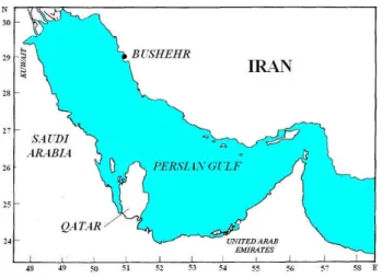
Figure1. Persian Gulf map (Ramesht 1988)

Figure2. Hourly time series of wind direction (UD) against time (24h interval)

Fig. 1. Persian Gulf map (Ramesht, 1988).Figure1. Persian Gulf map (Ramesht 1988)

Figure2. Hourly time series of wind direction (UD) against time (24h interval)

Fig. 2. Hourly time series of wind direction (U D) against time

(24-h interval).

ones, the wavelength and period of the swells gradually in-crease with time and distance from the source. Swells de-crease in amplitude, due to spreading and friction, so they are usually linear, coherent and have small-amplitude. Varia-tion of swell periods is between 8–12 s, but that of sea waves is between 1.5–5 s (Brockwell and Davis, 1996).

2 Study area and data sources

The Persian Gulf is a shallow, semi-enclosed sea and its cli-mate is arid, due to the excess of evaporation over precipita-tion and river run-off. The high evaporaprecipita-tion and saline water lead to anti-estuary circulation through the Hormuz Strait. The area of Persian Gulf is about 2.26×105km2, with an av-erage depth of 35 m.

All measurements were made at Bushehr (28◦₅₉0_N

50◦₅₀0_{E). Figure 1 shows the map of the study area. We have}

used the hourly time series wave and wind data measured by the Ports and Shipping Organization of Iran.

Wind parameters were measured at the coastal station in Bushehr and wave parameters were measured by a buoy (S4 model) at 29◦2012” N, 50◦39010” E, 12 km from the Bushehr coast, where the water depth is 15 m, and the coastal line direction is NW−SE.

Figure3. Hourly time series of wind speed (U10) against time (24h interval)

Figure4. Hourly time series of onshore wind against time (24h interval)

Figure5. Hourly time series of along shore wind against time (24h interval) Fig. 3. Hourly time series of wind speed (U10) against time (24-h

interval).

Wave characteristics are often measured by means of sub-merged pressure transducers. The use of this instrument im-poses some problems, the most important being the bias of its output due to the dynamical effect of the relative motion of water particles.

The usual analysis of zero-up crossing properties in a wave record requires digitization of the record at a finite sampling rate. Always in this buoy, large wave heights could be deter-mined with relative errors of 0.5% for 1/Tavg<1/20, where

1represents the sampling time interval and Tavgis the

spec-tral mean period. Other errors include statistical, numerical, sea state bias and the assumption of linear wave theory. Usu-ally the errors do not depend on the depth of the sea, and are greater for higher wave numbers. The errors are greater for a high sea state.

3 Wind characteristics in the area

One-hourly time series of wind direction and wind speed ob-served during the 21-day period (15 July–4 August 2000) are shown in Figs. 2 and 3. Wind data were recorded by the stan-dard buoy, whereas wave parameters were obtained from the raw data with hourly intervals. Data were recorded continu-ously. It should be mentioned that, although the predominant wind is NW-SE wind (shamal), the data we used are due to temporal (summer) wind (Ramesht (1988)).

In Fig. 2 the direction of wind (U D) shows variations be-tween 0◦and 330◦. This is in agreement with the climatolog-ical data available from the meteorologclimatolog-ical stations for the northern coast of the Persian Gulf. Figure 3 shows that the wind speed at 10 m above sea level (U10)varies between 0.34

and 10.83 ms−1_{with a characteristic diurnal oscillation. The}

lowest wind speed occurred about midnight and the highest speed around noon. The markings on the time-axis are made at 24-h intervals (starting on 15 July), in order that the diurnal pattern can be easily discernible.

In Figs. 4 and 5 wind speed is resolved into two compo-nents, along and across the shore. In Fig. 4 positive (nega-tive) values indicates a sea (land) breeze. These figures show that the sea breeze occurs during the day and the land breeze occurs at nighttime.

(4)

A. Parvaresh et al.: Statistical analysis of wave parameters in the north coast of the Persian Gulf 2033 Figure3. Hourly time series of wind speed (U10) against time (24h interval)

Figure5. Hourly time series of along shore wind against time (24h interval)

Fig. 4. Hourly time series of onshore wind against time (24-h

inter-val).

Figure3. Hourly time series of wind speed (U10) against time (24h interval)

Figure5. Hourly time series of along shore wind against time (24h interval) Fig. 5. Hourly time series of along shore wind against time (24-h

interval).

The diurnal variations of wind characteristics in this area, especially near the coastal zone, are normally attributed to land and sea breeze effects. Wind speed associated with the land-sea breeze is less than 6 m/s, but that of the sea-land breeze is greater. The change in wind speed and direction is almost simultaneous.

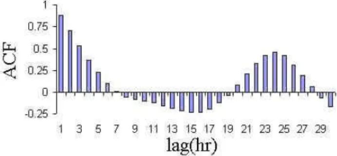
In this study, autocorrelation coefficients of wind speed data are calculated. These coefficients, with hourly intervals, are plotted versus time, in Fig. 6. Autocorrelation coeffi-cients for a lag of 1 to 5 h are greater than 0.5. Between lag 8 to 19 h the autocorrelation function is negative. The physical reason for this phenomenon is the air-sea temperature differ-ence. During the day the land temperature is greater than the water temperature, so the local wind is directed onshore in the direction of lower surface pressure. At night, the water temperature is less than the land temperature, but the magni-tude of the difference is less and the land-sea breeze is weak. Figure 6 shows that the autocorrelation function has a min-imum and a maxmin-imum at lag 15 and a maxmin-imum at lag 24. The minimum occurs when the maximum inverse correlation between the sea-land and the land-sea breeze happens. The maximum on lag 24 shows a diurnal cycle in the wind speed.

Figure6. Wind speed auto correlation function against time.

Fig. 6. Wind speed autocorrelation function against time.

Figure6. Wind speed auto correlation function against time.

Figur7. Hourly time series significant wave height (Hs), maximum wave height (Hm), wave period corresponding to Hm(Tm) and zero crossing period (Tz),.

Fig. 7. Hourly time series significant wave height (Hs), maximum wave height (Hm), wave period corresponding to Hm(Tm)and zero crossing period (Tz).

4 Wave characteristics

The time series of wave parameters are shown in Fig. 7. In this figure the significant wave height, Hs, is defined as the

(5)

2034 A. Parvaresh et al.: Statistical analysis of wave parameters in the north coast of the Persian Gulf Figur7. Hourly time series significant wave height (Hs), maximum wave height (Hm),

wave period corresponding to Hm(Tm) and zero crossing period (Tz),.

Figure8. Wave age (C/U10) vs. wave steepness (Hs/L)

Figure9. Variation of cross- correlation for wind speed (U10) and significant wave height (Hs) with time-lag

Fig. 8. Wave age (C/U10)vs. wave steepness (Hs/L).

Figur7. Hourly time series significant wave height (Hs), maximum wave height (Hm), wave period corresponding to Hm(Tm) and zero crossing period (Tz),.

Figure8. Wave age (C/U10) vs. wave steepness (Hs/L)

Figure9. Variation of cross- correlation for wind speed (U10) and significant wave height (Hs) with time-lag

Fig. 9. Variation of cross-correlation for wind speed (U10) and

sig-nificant wave height (Hs) with time-lag.

mean of the highest one-third of the waves present in the sea and the maximum wave height, Hm, is the maximum vertical

distance between the highest crest to the lowest trough; Tm

is the wave period corresponding to Hm, and Tzis the mean

zero-up crossing period of the wave field. As is seen, each of these parameters varies between 0.10 to 1.02 m; 0.15 to 1.70 m; 3.56 to 4.59 s and 3.57 to 5.255 s, respectively. Thus, the prevailing wave conditions mostly reflect the sea state 2 and 3 codes (WMO 1988) during the observation period.

The dimensionless wave parameters, namely, the wave steepness (Hs/L) and the wave age (C/U10), where C is

the phase speed, are often used to determine the nature of the sea state. Wave steepness is usually expressed as the ra-tio between the significant wave height and the wave length, of the peak period. Thompson et al. (1984) gave a classifi-cation scheme for ocean waves based on (Hs/L) criterion –

namely, sea young swell, mature swell and old swell. Ac-cording to their classification, locally generated waves or sea waves have steepness values greater than 0.025. Figure 8 does not show any correlation between wave age and wave steepness. This figure mainly reflects local waves or sea waves as (Hs/L) is greater than 0.025. Younger waves are

steeper than the older ones (Thompson et al., 1984).

5 Statistical correlation between wave and wind param-eters

Statistical correlations obtained among various analysed wave parameters and wind speed are given in Table 1. Wave

Table 1. Correlation coefficients of the analysed wave parameters

and wind speed.

U10 Hs Hm Havg Tz Tm U10 0.376 0.373 0.375 0.297 0.295 Hs 0.999 0.998 0.675 * Hm 0.998 0.671 * Havg 0.670 * Tz 0.996

* Indicates that the correlation coefficient values are not statistically significant.

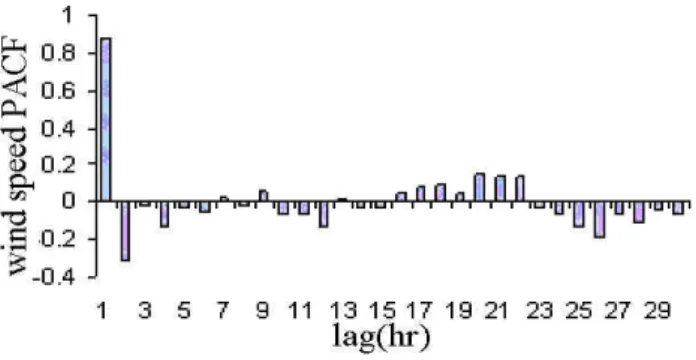
Figure10. Wind speed partial auto correlation with 1hr time lag

Figure11. Predicted (solid line) and measured (dotted line) wind speed(U4.5)

Figure12. Significant wave height auto correlation with 1hr time lag Fig. 10. Wind speed partial autocorrelation with 1-h time lag.

heights (Hs and Hm) and wave periods (Tz and Tm) show

positive and low correlation against wind speed (U10).

Positive correlation in wind speed (U10) against Hs and

Hmis due to the increase of wind energy. Low correlation

coefficients are perhaps due to the diurnal change in wind di-rection. When the wind direction varies with time, the role of wind speed on the wave height growth decreases. When the wind and wave directions are opposite from each other, the wind speed applies an opposing stress against the waves and therefore the wave height growth is negative. So in this area the correlation between wind speed and wave height is weak. The correlation between onshore and along-shore wind speed and wave parameters is weak as well.

The positive correlation of wave periods with wind speed, which is observed in this case, reveals the complex nature of the wave period evolution during the active wave growth con-ditions. Hmshows a better correlation with U10than Tm. The

correlation coefficient values obtained for Tmagainst Hs and

Hmare not shown in Table 1, since they are not statistically

significant.

A strong positive correlation (corr. coeff.=0.999) exists between Hs and Hm. The concept of statistically

statio-nary wave heights was originally proposed by Longuet-Higgins (1952). According to this concept, the ratios of sig-nificant wave parameters (statistical averages) are expected to be constant. The theoretical value proposed for Hm/Hsis

1.53 (Longuet-Higgins, 1952). Our analyses show that this ratio is 1.66. John (1985) suggested that Hm/Hs obtained

(6)

A. Parvaresh et al.: Statistical analysis of wave parameters in the north coast of the Persian Gulf 2035

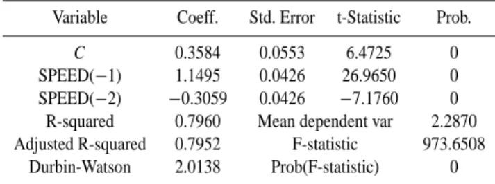
Table 2. Statistical coefficient of wind speed time series model.

Variable Coeff. Std. Error t-Statistic Prob.

C 0.3584 0.0553 6.4725 0 SPEED(−1) 1.1495 0.0426 26.9650 0 SPEED(−2) −0.3059 0.0426 −7.1760 0

R-squared 0.7960 Mean dependent var 2.2870 Adjusted R-squared 0.7952 F-statistic 973.6508

Durbin-Watson 2.0138 Prob(F-statistic) 0

Table 3. Statistical coefficient of significant wave height time series

model.

C 0.0089 0.0039 2.2774 0

Hs(−1) 0.9676 0.0140 68.8966 0 R-squared 0.9045 Mean dependent var 0.2300 Adjusted R-squared 0.9043 F-statistic 4746.745 Durbin-Watson stat 1.9538 Prob(F-statistic) 0

important to note that the length of the time series used for the wave analysis, as well as the differences in the wave mea-suring devices employed, may lead to the differences in the wave statistics derived from a given wave record. Our re-sults generally agree with the Rayleigh distribution law. We have found H1/10/Hsto be 1.271 comparable to the Rayleigh

value of 1.275.

An important question is whether the waves begin grow-ing when the sea-land breeze begins or whether a lag time (τ ) exists between these two. From simple physical considera-tions one can safely assume a certain lag time for waves to grow as wind starts blowing over the sea surface. Therefore, we computed the cross-correlation between U10and Hs. The

time history of any two sets of the time series records can be tested to know the general dependence of one set of data on the other (Bendat and Piersol, 1986).

Cross-correlation function Ruh, between U10 and Hs, is

defined as:

Ruh=lim(1/T )

Z

U10×Hs(τ + t )dt , (1)

where T is the total duration of the time series record and τ is the time lag (Box and Jenkins, 1976). This function is plotted in Fig. 9 and reveals two peaks. The primary peak is between the lag of 3 to 11 h and the second one at 32 h. The Ruh

val-ues for these peaks are 0.41 and 0.12, respectively. The sec-ond peak could be due to the presence of diurnal variability in the data (24+(4+11)/2∼32). The first peak suggests that the wave field lags behind the wind by at least about 3 h. The constant value of Ruhbetween lag 4 to lag 11 is the result of

the variation of the wind direction in this area.

Figure12. Significant wave height auto correlation with 1hr time lag

Fig. 11. Predicted (solid line) and measured (dotted line) wind

speed (U4.5).

Figure12. Significant wave height auto correlation with 1hr time lag Fig. 12. Significant wave height autocorrelation with 1-h time lag.

6 Prediction of wind and wave parameters by time se-ries modeling

In this section the statistical models used will be de-scribed. The theoretical background described and the tech-niques used are presented. Consider the time series {Xt, :

t =0, ±1, ±2, ...}, i.e. a sequence of dependent random vari-ables in time. The time series is stationary if

F (Xt1, Xt2, . . .Xtn) = F (Xt1+k, Xt2+k, . . ., Xtn+k), (2)

where n, k, t1, t2,. . . tn, are integer numbers and F (.)

rep-resents the joint probability distribution function of any n random variables of process {Xt}. The time series is said

to be weakly or second-order stationary, if the mean func-tion is constant and the covariance between any two of them just depends on the time difference between them but not on time itself (γt,t −k=γ0,k). An important example of a

weakly stationary process is the white noise (at) process,

which is defined as a sequence of independent, identical dis-tribution of random variables. We shall usually assume that the white noise has a zero mean and denote its variance as (σ_a2

t) (Guedes Soares and Ferreira, 1996).

If the time series Xt verifies a relation

Xt =ϕ1Xt −1+ϕ2Xt −2+ · · ·ϕpXt −p+ (3)

at−θ1at −1−θ2at −2− · · ·θqat −q,

where φ1, φ2, . . . , φp, θ1, θ2, . . . , θqare unknown constants,

it is said to be described by an ARMA model of order p and

q, respectively, where the time series should be stationary and {at, : t =0, ±1, ±2, . . .} should be a white noise process.

(7)

Figure13. Significant wave height partial auto correlation with 1hr time lag

Figure14. Predicted (solid line) and measured (dotted line) significant wave height

Figure15. Dominant wave period Tp auto correlation with 1hr time lag Fig. 13. Significant wave height partial autocorrelation with 1-h

time lag.

Figure15. Dominant wave period Tp auto correlation with 1hr time lag

Fig. 14. Predicted (solid line) and measured (dotted line) significant

wave height.

called the moving average of order q−MA(q)− and when the order q is zero it becomes an autoregressive of order

p−AR(p).

A time series Xt is said to follow an ARIMA if the dth

difference Wt=1dXt is a stationary ARMA process. If Wt

is ARMA(p, q), we say that Xt is ARIMA(p, d, q).

Dif-ferences can also be conveniently written in terms of B, as a backshift operator, i.e. 1d=(1−B)d. The ARIMA model is then expressed as

8(B)(1 − B)dXt =2(B)at, (4)

where 8(B) and 2(B) are:

8(B) =1 − ϕ1B − ϕ2B2· · ·ϕpBp (5)

2(B) =1 − θ1B − θ2B2· · ·θpBp. (6)

Fundamental tools in time series analyses are the autocor-relation function (ACF), ρk, and the partial autocorrelation

function (PACF), φkk, where ρkand φkkare:

ρk= cov(Xt, Xt +k) √ var(Xt)pvar(Xt +k) =γk γ0 (7) φkk = cov((Xt −Xt), (Xt +k−Xt +k)) p var(Xt −Xt) q var(Xt +k−Xt +k) , (8)

respectively, and Xt stands for the best linear estimate of Xt

and subscript t stands for X value in time t . (Guedes Soares and Ferreira, 1996; Hidalgo et al., 1995).

Figure15. Dominant wave period Tp auto correlation with 1hr time lag Fig. 15. Dominant wave period Tpautocorrelation with 1-h time lag.

Figure16. Dominant wave period Tp partial auto correlation with 1hr time lag

Figure17. Predicted (solid line) and measured (dotted line) (1-B) 2Tp

Fig. 16. Dominant wave period Tppartial autocorrelation with 1-h time lag.

In this study we have examined whether the time series of wind speed, significant wave height, and wave period, are stationary. These parameters are modeled by ARMA and ARIMA models. We have used Eviews software and the time series have been evaluated by the Dickey-Fuller unit root test. This test on wind speed data shows that this time series is stationary at 99% level. We have plotted ACF and PACF of wind speed data in Figs. 6 and 10. These figures show that the behavior of this time series is autoregressive, AR. By re-gression test on all lags, we found that the best predicted level relates to lags 1 and 2 h. Adding other lags on regression has no effect on the prediction level. Adding moving average coefficients in this case is not efficient. Therefore, the best model in this case is autoregressive, AR. Coefficients of this model are given in Table 2. The table shows the following relation, with a prediction level of 79.6%:

Ut =0.358 + 1.149Ut −1−0.305Ut −2, (9)

where Ut stands for the wind speed at time t(h). The

pre-dicted and measured wind speeds are shown in Fig. 11. The Dickey-Fuller unit root test on significant wave height

Hs shows that the significant wave height time series is

sta-tionary at the 95% level. ACF and PACF of this time series are plotted in Figs. 12 and 13, respectively. Regressions on all lags indicate that the best model for the Hs time series is:

Hs,t(m) =0.0089 + 0.976Hs,t −1(m). (10)

The predicted and measured significant wave heights are shown in Fig. 14. The statistical coefficients of this time se-ries model are shown in Table 3.

(8)

A. Parvaresh et al.: Statistical analysis of wave parameters in the north coast of the Persian Gulf 2037 The Dickey-Fuller unit root test on dominant period Tp

shows that Tp time series is stationary at 99% level. ACF

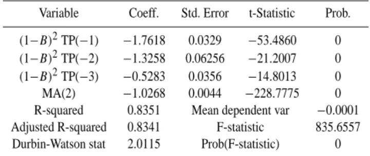
and PACF of this time series are shown in Figs. 15 and 16. The best prediction level of the ARMA model for this time series is 20% level, and therefore the ARIMA model should be used for this time series. Using the ARIMA test for this time series, we found that the best model for this time series is:

(1 + 1.761B + 1.325B2+0.5283B3)(1 − B)2T pt

= −1.02ut −2, (11)

where ut −2 is the residual of two back lags, ut stands for

at and Tpis the most probable period of the wave field. This

model predicts Tpat the 83.52% level. Statistical coefficients

of this model are shown in Table 4. The predicted and mea-sured values of (1−B)2Tpare shown in Fig. 17.

7 Conclusions

1. Observed winds (U10) behave as land and sea breezes,

with the minimum speed occurring around midnight and the maximum around noon. The wind speed varied from 0.34 to 10.38 m/s.

2. Observed significant wave height (Hs) and mean

zero-up crossing period (Tz) varied from 0.1 to 1.02 m, and

3.56 to 4.95 s respectively. The wave conditions mostly reflect sea states 2 and 3 (WMO code).

3. Due to continuous variations of wind speed with time, correlations between wind speed and wave parameters show low values.

4. The wave height distribution follows the Rayleigh dis-tribution law. The ratio of Hs/Hm obtained with the

present data is 1.75.

5. Wave conditions mostly reflect local waves or sea waves.

6. There is no correlation between wave age and wave steepness. This is due to the fact that the wave never ages during the diurnal wind cycle. The waves are local waves.

7. Cross correlation of U10and Hs reveals that waves lag

behind wind by about 4 h.

8. The time series of the wind speed (U10), significant

wave height (Hs) and dominant wave period (Tp) are

stationary at level 99%, 95% and 99%, respectively. The best model and the prediction level of these param-eters are:

Ut =0.358 + 1.149Ut −1−0.305Ut −2 R2=79.6% Hs,t (m) =0.0089 + 0.976Hs,t −1(m) R2=90.4% (1 + 1.761B + 1.325B2+0.5283B3)(1 − B)2Tp,t

= −1.02Ut −2 R2=83.5%

Table 4. Statistical coefficient of dominant period Tp time series

model.

(1−B)2TP(−1) −1.7618 0.0329 −53.4860 0

(1−B)2TP(−2) −1.3258 0.06256 −21.2007 0

(1−B)2TP(−3) −0.5283 0.0356 −14.8013 0 MA(2) −1.0268 0.0044 −228.7775 0 R-squared 0.8351 Mean dependent var −0.0001 Adjusted R-squared 0.8341 F-statistic 835.6557 Durbin-Watson stat 2.0115 Prob(F-statistic) 0 Figure16. Dominant wave period Tp partial auto correlation with 1hr time lag

Figure17. Predicted (solid line) and measured (dotted line) (1-B) 2Tp

Fig. 17. Predicted (solid line) and measured (dotted line) (1−B)2Tp.

Acknowledgements. The authors wish to thank the office of

Gradu-ate Studies of the University of Isfahan for their support. We would like to thank the Ports and Shipping Organization of Iran for the wave data.

Topical Editor N. Pinardi thanks two referees for their help in eval-uating this paper.

References

Atkinson, B. W.: Meso-scale atmospheric circulation, Academic press, London, 495, 1981.

Bendat, J. S. and Piersol, A. G.: Random Data: Analysis and Mea-surement Procedures, John Wiley and Sons, 566, 1986. Box, G. E. P and Jenkins, G. M.: Time series analysis forecasting

and control, San Fransisco, Holden Day, 1976.

Brockwell, P. J. and Davis, R. A.: Introduction to Time Series and Forecasting, Springer, New York, 1996.

Guedes Soares, C. and Ferreira, A. M.: Representation of non-stationary time series of significant wave height with autoregres-sive models, Probabilistic Engineering Mechanics, 11, 139–148, 1996.

Hidalgo, O., Nieto, J. C., Cunha, C., and Guedes Soares, C.: Filling missing observations in time series of significant wave height, in: Proceedings of the 14th International Conference on Offshore Mechanics and Arctic Engineering, edited by: Guedes Soares, C., vol. II ASME, New York, 9–17, 1995.

Hsu, S. A.: Coastal Meteorology, Academic Press, New York, 1988. Inoue, T.: On the Growth of the Spectrum of a Wind Generated Sea According to a Modified Miles-Phillips Mechanism and its Ap-plication to Wave Forecasting, Geophysical Sciences Laboratory Report No. TR-67-5, Department of Meteorology and Oceanog-raphy, New York University, 1967.

(9)

John, V. C.: Distributions and relationships of height and period of ocean waves off Mangalore, Indian Jornal of marine Sciences, 6, 49–50, 1985.

Longuet-Higins, M. S.: On the statistical distribution of the heights of the sea waves, Journal of Marine Research, 11, 3, 245–266, 1952.

Ramesht, M. H.: Persian Gulf geography, Isfahan University Press, 1988.

Thompson., T. S., Nelson, A. R., and Sedivy, D. G.: Wave group anatomy, Proceeding of 19th conference on Coastal engineering, American Society of Civil Engineers, 1, 661–677, 1984. WMO: Guide to wave analysis and forecasting, No. 702, Secretariat