HAL Id: insu-01965223
https://hal-insu.archives-ouvertes.fr/insu-01965223
Submitted on 13 Jan 2021
HAL is a multi-disciplinary open access
archive for the deposit and dissemination of
sci-entific research documents, whether they are
pub-lished or not. The documents may come from
teaching and research institutions in France or
abroad, or from public or private research centers.
L’archive ouverte pluridisciplinaire HAL, est
destinée au dépôt et à la diffusion de documents
scientifiques de niveau recherche, publiés ou non,
émanant des établissements d’enseignement et de
recherche français ou étrangers, des laboratoires
publics ou privés.
PAN
Bruno Franco, Lieven Clarisse, T. Stavrakou, Jean-François Müller, M.
Van damme, S. Whitburn, Juliette Hadji-Lazaro, Daniel Hurtmans,
Domenico Taraborrelli, Cathy Clerbaux, et al.
To cite this version:
Bruno Franco, Lieven Clarisse, T. Stavrakou, Jean-François Müller, M. Van damme, et al.. A general
framework for global retrievals of trace gases from IASI: Application to methanol, formic acid and
PAN. Journal of Geophysical Research: Atmospheres, American Geophysical Union, 2018, 123 (24),
pp.13,963-13,984. �10.1029/2018JD029633�. �insu-01965223�
Journal of Geophysical Research: Atmospheres
A General Framework for Global Retrievals of Trace Gases
From IASI: Application to Methanol, Formic Acid,
and PAN
B. Franco1 , L. Clarisse1 , T. Stavrakou2 , J.-F Müller2 , M. Van Damme1 , S. Whitburn1 , J. Hadji-Lazaro3, D. Hurtmans1, D. Taraborrelli4 ,C. Clerbaux1,3 , and P.-F Coheur1
1Université libre de Bruxelles (ULB), Service de Chimie Quantique et Photophysique, Atmospheric Spectroscopy, Brussels,
Belgium,2Royal Belgian Institute for Space Aeronomy, Brussels, Belgium,3LATMOS/IPSL, Sorbonne Université, UVSQ,
CNRS, Paris, France,4Institute of Energy and Climate Research, Forschungszentrum Jülich GmbH, Jülich, Germany
Abstract
Retrieving concentrations of minor atmospheric trace gases from satellite observations is challenging due to their weak spectral signature. Here we present a new version of the ANNI (Artificial Neural Network for Infrared Atmospheric Sounding Interferometer, IASI) retrieval framework, which relies on a hyperspectral range index (HRI) for the quantification of the gas spectral signature and on an artificial feedforward neural network to convert the HRI into a gas total column. We detail the different steps of the retrieval method, especially where they differ from previous work, and apply the retrieval to three important volatile organic compounds: methanol (CH3OH), formic acid (HCOOH), and peroxyacetyl nitrate (PAN).The comparison of the retrieved columns with those from an optimal estimation inversion retrieval shows an overall excellent agreement: differences occur mainly when the sensitivity to the target gas is low and are consistent with the conceptual differences between the two approaches. We present retrieval examples over selected regions, comparison with previously developed products, and the global seasonal distributions including the first global distributions of PAN on a daily basis. The ANNI retrieval has been carried out on the whole time series of IASI observations (2007–2018), so that currently over 10 years of twice-daily global CH3OH, HCOOH, and PAN total column distributions have been produced. This unique
data set opens avenues for tackling important questions related to sources, transport, and transformation of volatile organic compounds in the global atmosphere.
Plain Language Summary
Volatile organic compounds are atmospheric trace gases of various origins (e.g., biogenic, anthropogenic, and biomass burning). For many of them, their sources, removal processes, and impacts on atmosphere and climate are not well understood. One major reason for this is the paucity of measurements of their concentration. In this study, we describe the innovative ANNI (Artificial Neural Network for Infrared Atmospheric Sounding Interferometer, IASI) method that allows us to calculate here the abundance of three important volatile organic compounds (methanol, formic acid, and peroxyacetyl nitrate) from infrared measurements of the Earth’s surface and atmosphere performed by the IASI satellite instrument. The method consists of two steps. First, the spectral signature, associated with the trace gas of interest, is extracted from the observed spectrum. The second step relies on an artificial neural network to transform the observed signature into a gas abundance. This technique provides a high level of sensitivity and accuracy compared with conventional physical methods. Furthermore, its computational efficiency makes it possible to readily process all the measurements (over 1,200,000/day) recorded since the launch of IASI in 2006. The result is a unique day-to-day global picture of the three gases, which represents a benchmark for tackling their uncertainties.1. Introduction
As one of the most emitted and abundant volatile organic compounds (VOCs) in the Earth’s atmosphere, methanol (CH3OH) affects tropospheric hydroxyl radical (OH) concentrations through its photochemical degradation and contributes to the production of carbon monoxide, formaldehyde, and tropospheric ozone (O3; e.g., Duncan et al., 2007; Millet et al., 2008; Singh et al., 2001; 1995; Stavrakou et al., 2011; Tie et al., 2003;
Wells et al., 2014). Formic acid (HCOOH) is the most abundant carboxylic acid in the troposphere, with a
RESEARCH ARTICLE
10.1029/2018JD029633
Key Points:
• A general framework is presented for a flexible, robust, and computationally efficient retrieval of trace gases from infrared satellite spectra
• The scheme is applied to retrieve daily global distributions of CH3OH, HCOOH, and PAN columns on a year of IASI observations
• Retrieval results are consistent with those obtained with an optimal estimation inversion Supporting Information: • Supporting Information S1 Correspondence to: B. Franco, [email protected] Citation:
Franco, B., Clarisse, L., Stavrakou, T., Müller, J.-F., Van Damme, M., Whitburn, S., et al. (2018). A general framework for global retrievals of trace gases from IASI: Application to methanol, formic acid, and PAN. Journal of Geophysical Research: Atmospheres, 123, 13,963–13,984. https://doi.org/10.1029/2018JD029633
Received 13 SEP 2018 Accepted 16 DEC 2018
Accepted article online 20 DEC 2018 Published online 28 DEC 2018
©2018. American Geophysical Union. All Rights Reserved.
significant influence on atmospheric acidity and thus on pH-dependent processes in cloud droplets, especially in remote environments (Chameides & Davis, 1983; Galloway et al., 1982; Jacob, 1986; Keene et al., 2015; Millet et al., 2015; Stavrakou et al., 2012; Yu, 2000). Peroxyacetyl nitrate (CH3C(O)O2NO2), abbreviated as PAN, is
con-sidered to be the largest, thermally unstable tropospheric reservoir for nitrogen oxide radicals (NOx= NO + NO2), enabling their redistribution from source to remote regions where it favors tropospheric O3production (Fischer et al., 2011, 2014; Kasibhatla et al., 1993; Moxim et al., 1996; Wang et al., 1998).
These VOCs have various primary and/or secondary sources, including terrestrial vegetation, oceans, biomass burning, anthropogenic emissions, and the oxidation of other VOCs. Large uncertainties in their atmospheric budget estimates still exist (e.g., Fischer et al., 2014; Millet et al., 2008, 2015; Stavrakou et al., 2011, 2012; Wells et al., 2014), mainly because of the paucity of VOC observations, in particular, in remote and tropical regions. Better constraints on the respective sources and sinks of VOCs are clearly needed to quantify their impact on atmospheric oxidants, on methane lifetime, and consequently on climate.
Hyperspectral satellite sensors probing the atmosphere in the thermal infrared can play a major role in reduc-ing these uncertainties by providreduc-ing global observations of VOCs. Limb sounders like ACE-FTS (Atmospheric Chemistry Experiment-Fourier Transform Spectrometer) and MIPAS (Michelson Interferometer for Passive Atmospheric Sounding) can provide CH3OH, HCOOH, and PAN measurements in the upper troposphere-lower
stratosphere (UTLS; Dufour et al., 2006, 2007; Glatthor et al., 2007; González Abad et al., 2009; Grutter et al., 2010; Moore & Remedios, 2010; Pope et al., 2016; Rinsland et al., 2006, 2007; Tereszchuk et al., 2013; Wiegele et al., 2012). Nonetheless, their geometry prevents the sampling of the lowest altitudes and hence does not allow direct investigation of VOC emissions and other processes affecting the bulk of their atmospheric con-tent, which resides in the lower troposphere. The nadir-viewing TES (Tropospheric Emission Spectrometer) satellite sensor probes the low troposphere and allows retrieval of CH3OH, HCOOH, and PAN (e.g., Alvarado et al., 2011; Beer et al., 2008; Cady-Pereira et al., 2014, 2012; Payne et al., 2014, 2017; Shephard et al., 2015; Wells et al., 2012). However, sounders embarked on meteorological platforms offer a denser spatial sampling, more suitable for investigating the spatial heterogeneity and short-term evolution of highly variable VOCs. Here we use the observations of the nadir-looking IASI (Infrared Atmospheric Sounding Interferometer) satel-lite sensor (Clerbaux et al., 2009), operating on the Metop platforms, which offers key advantages for studying VOCs, their variability and evolution: (1) a twice-daily global coverage (∼9:30 morning and evening) owing to the wide swath of the sounder combined with an intensive spatial sampling (over 1,250,000 spectra recorded per day), (2) a high spatial resolution (pixel size of 12 km at nadir), (3) an extensive and continuous coverage of the thermal infrared (645–2,760 cm−1) where many VOCs are optically active, at good spectral resolution
(0.5 cm−1 apodized) and with low noise, and (4) the availability of 10 years of continuous measurements,
offering a consistent and unique observational data set of the global atmosphere.
Whereas the detection of the VOC spectral signature in the IASI spectra is relatively simple, the retrieval of concentrations is challenging. Physical retrieval methods relying on an iterative fit of the observed spectra allow for accurate and fully characterized measurements, but their implementation for minor, highly vari-able trace gases is nontrivial. In addition, the production of associated multiyear satellite data sets using such methods is computationally demanding. Therefore, straightforward retrieval strategies have been developed in the past, which allowed producing the first global maps of CH3OH, HCOOH, and ammonia (NH3; Clarisse et al., 2009; Pommier et al., 2016; Razavi et al., 2011). These retrievals consisted of calculating brightness tem-perature differences (dBT) which were converted into total columns using constant multiplicative factors or two-dimensional look-up tables. Nonetheless, these products have limitations in terms of reliability and error characterization, which are not easily addressed. Although IASI measurements of PAN have been reported in concentrated biomass burning and pollution plumes (Clarisse, Fromm, et al., 2011; Clarisse, R’Honi, et al., 2011; Coheur et al., 2009), and PAN TES data have been used to study Northern Eurasian and North American fires, long-range pollution transport, and year-to-year variations in the Tropics (Fischer et al., 2018; Jiang et al., 2016; Payne et al., 2017; Zhu et al., 2015, 2017), no global daily distributions of PAN have been retrieved until now. In this study, we present an innovative fast retrieval methodology that provides more sensitive VOC columns from IASI, with a better error characterization. This methodology builds on the retrieval approach recently developed for NH3(Van Damme et al., 2017; Whitburn et al., 2016), for which the main concepts and different steps of the retrieval are illustrated in Figure 1. In brief, the retrieval itself (red boxes in Figure 1) relies on two computational steps:
Journal of Geophysical Research: Atmospheres
10.1029/2018JD029633
Figure 1. Conceptual flowchart of the ANNI (Artificial Neural Network for IASI) retrieval method of trace gases. IASI = Infrared Atmospheric Sounding Interferometer.
1. The calculation for each IASI observation of a hyperspectral range index (HRI). This quantity is a very sen-sitive, broadband spectral index that quantifies the signal strength of a target absorber in a radiance spectrum.
2. The conversion of the HRI into a total column abundance via an artificial feedforward neural network (NN). In addition to the HRI, the NN relies on a series of auxiliary parameters related to the state of the atmo-sphere and of the surface. Perturbations to the input data of the NN allows quantification of the uncertainties associated with single-pixel retrieved columns.
In addition, appropriate filtering of the data (before and after the retrieval) removes cloudy scenes and obser-vations with limited or no sensitivity to the target trace gas. Finally, a calibration offset is added to the retrieved
columns to account for the constant, climatological background column of the target gas in the atmosphere (green box in Figure 1; see section 4.2).
While the retrieval itself is simple and fast, the initial setup (blue and red boxes in Figure 1) of the HRI and NN is nontrivial. In particular, both rely on weight constants that must be determined with care beforehand from a data set of real (for the HRI) and synthetic (for the NN) IASI spectra. The setup of the HRI and NN and the training of these weight constants are detailed in sections 2 and 3 below. In section 4, we compare the new retrievals over selected regions with alternative retrievals obtained using an optimal estimation inversion. This not only allows demonstration of the robustness of the new products but also helps to illustrate the strengths and weaknesses of both retrieval approaches. Finally, for CH3OH and HCOOH these alternative retrievals are used to derive the aforementioned calibration offsets. In section 5, we present—where relevant—comparisons with previous IASI-derived products, examples of column retrievals on individual overpasses, and seasonal climatologies of the different species.
The general retrieval framework described in this work can be considered to be the third version of the ANNI (Artificial Neural Network for IASI) retrieval, previously implemented for NH3(ANNI-NH3-v1 in Whitburn et al., 2016, and v2 in Van Damme et al., 2017). As detailed below, some of the changes were introduced to make the application of ANNI to VOCs possible. Others were introduced to improve the sensitivity, robustness and generalizability of the approach. While the focus of this paper is on CH3OH, HCOOH, and PAN, a new set of HRI
for NH3is also computed, which incorporates all the improvements that are introduced here. A forthcoming
study will be dedicated to the retrieval and evaluation of the new version (v3) of the ANNI-NH3product.
2. The HRI
Proposed by Walker et al. (2011), the HRI is a dimensionless index that quantifies the strength of the spectral signature of a target gas in an observed spectrum y:
HRI =K TS−1 y (y −̄y) √ KTS−1 y K 1 N (1)
where K is a spectral Jacobian, Sya covariance matrix, and̄y the mean spectrum generated from a representa-tive data set of background spectra associated with a climatological column of the target gas, and N an extra normalization factor (see section 2.2). The HRI is conveniently normalized to have a mean of zero and a stan-dard deviation of 1 when calculated on the data set of background spectra. The HRI is particularly suitable for the detection of highly variable infrared absorbers, like NH3, which are not observed in every spectrum. In this case, the climatological column amount is close to zero and the background spectra are those without observable signature of NH3.
The HRI can encompass spectral ranges of up to several hundreds per centimeter to exploit all the channels in which the target species is absorbing. This results in a substantial gain of sensitivity over other detection methods and makes it highly suitable for the detection of broadband absorption features, as demonstrated with the detection of a series of aerosol types in Clarisse et al. (2013). Therefore, the HRI can be successfully applied to VOCs, usually characterized in the thermal infrared by weak, sometimes broad absorption.
2.1. Choice of Spectral Ranges
Larger spectral ranges lead in principle to a more sensitive HRI. However, this is true only in the linear regime in which the covariance matrix describes a normal distribution. In practice, it can be advantageous to exclude spectral ranges where nonlinearity prevails. For instance, the spectral range 1,100–1,200 cm−1can exhibit
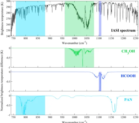
pronounced spectral surface emissivity features over deserts. In addition, it might be useful to avoid a spectral interval in which another species with a similar spectral signature is absorbing (this is particularly the case for broadband absorbers). The spectral ranges that were selected for CH3OH, HCOOH, and PAN are shown in
Figure 2 (in colored rectangles), on top of a typical IASI spectrum:
• The chosen spectral range for CH3OH (960–1,080 cm−1) encompasses its fundamental𝜈8 C–O stretching
Journal of Geophysical Research: Atmospheres
10.1029/2018JD029633
Figure 2. Typical IASI spectrum (displayed in brightness temperature) in the 750–1,250 cm−1spectral range (upper frame), and the JacobiansKof the CH3OH, HCOOH, and PAN spectral absorptions used for the calculation of the HRI (lower frames). The spectral ranges selected for the retrieval of each species are illustrated in colored rectangles. In the lower frames, the brightness temperatures were normalized to have a minimum value of−1 for visibility purposes. The JacobiansKhave been produced by the line-by-line radiative transfer model Atmosphit (Coheur et al., 2005) for a standard atmosphere. The IASI spectrum illustrated here has been recorded at 33.21∘N, 89.22∘W, on 15 July 2011 (∼9:30 UTC), at a viewing angleZof 37.09∘. IASI = Infrared Atmospheric Sounding Interferometer; PAN = peroxyacetyl nitrate.
HRI. Ozone abundances will therefore have to be accounted for specifically in the retrieval (see section 3.2). • For HCOOH, a narrow window (1,100–1,110 cm−1) was chosen around its𝜈16 Q branch.
• Two large bands centered at 794 cm−1(the𝜈16 NO
2stretch) and at 1,163 cm−1(the𝜈10 C–O stretch) can be
considered for PAN, but only the first one has been used here (760–880 cm−1) as the other range is more
affected by variations in the spectral surface emissivity.
• The range for NH3(812–1,126 cm−1; not shown in Figure 2) exploits the strongest lines from its𝜈2 vibrational
band and has been slightly reduced compared to the previous product (800–1,200 cm−1; Van Damme et al.,
2017; Whitburn et al., 2016) to minimize interferences.
2.2. Iterative HRI Calculation
The Jacobian K in equation (1) is the derivative of the radiance spectrum with respect to the column abun-dance of the target species. For each target species, a Jacobian (illustrated in the bottom panels in Figure 2) has been generated by the line-by-line radiative transfer model Atmosphit (Coheur et al., 2005) for a standard atmosphere (upper blue box in Figure 1). The vertical concentration profiles for CH3OH, HCOOH, and PAN
orig-inate from averaged volume mixing ratio profiles derived from WACCM v6 (Whole Atmosphere Community Climate Model; see, e.g., Chang et al., 2008) simulations over the 1980–2020 period.
For each target species, the HRI calculation also depends on a generalized covariance matrix Syand an asso-ciated background spectrum̄y. The covariance matrix determines the weight of each spectral channel, and ideally expresses the variability and covariance of all interfering species, but explicitly not that of the target species (Walker et al., 2011). Such a matrix can be obtained from a representative set of IASI spectra with a constant, climatological column amount of the target species. For short-lived trace gas absorbers like NH3,
the pair (Sy,̄y) can straightforwardly be constructed from spectra with no observable signature of the gas (the associated climatological column is then close to zero). To select such spectra, an iterative approach was
followed (Clarisse et al., 2013). First, a representative set of IASI spectra was built, consisting of all the spectra from the fifteenth of each month of 2013 but sampled to yield a spatially uniform distribution (to avoid over-representing polar regions). This whole set was then used for the generation of a first (Sy,̄y) pair. This allowed the production of a first set of HRI, which in turn was used to remove the spectra with detectable signatures of the trace gas (typically with an HRI above 3 or 4; see below). The reduced set of spectra allows the calcula-tion of a better (Sy,̄y) pair. Repeating this process several times (typically 10 iterations) leads to convergence of the set of spectra, of the corresponding (Sy,̄y), and of the HRI.
In the current study, it was found that a more sensitive HRI could be constructed by considering only the spec-tra with an HRI below 1–1.5. Using such a low threshold removes much more specspec-tra, including those with spectral signatures barely above the instrumental noise and even spectra without detectable gas quantities (this is obvious for NH3, where spectra above remote oceans frequently exhibit HRIs below 1). Nevertheless,
removing such spectra leads to a more sensitive HRI and does not generate anomalies (e.g., false detections). There is, however, a side effect, in that the initial normalization of the HRI is not preserved in the iterative pro-cess. This is the reason why an additional normalization factor (N) is needed in equation (1). Note that this factor N needs to be recalculated at each iteration. For NH3, the normalization factor N was calculated as the
standard deviation of the HRI over a remote ocean area, where no NH3is expected. The HRI as described above
is more sensitive than the HRI of NH3used in previous work. In addition, a weak H2O dependence observed
especially over oceans in the old HRI is no longer observed in the new HRI.
The procedure outlined above for NH3was carried out in almost exactly the same way for the VOCs.
How-ever, as these species are longer lived with typical atmospheric lifetimes of a few days for HCOOH and CH3OH
(Stavrakou et al., 2011, 2012) and even longer for PAN in the upper troposphere (Fischer et al., 2014), nonneg-ligible concentrations are found even at the most remote locations. Hence, the set of spectra on which the (Sy,
̄y) are based converges to a set where a weak spectral signature of the target gas remains. For these species,
an HRI of zero therefore no longer corresponds to the absence of the trace gas. This fact has implications for the actual retrieval, which are discussed in section 4.2. Note that the normalization region for the VOCs was taken over the remote ocean between 180–130∘W and 60–10∘S. Figure 3 illustrates for the three species the mean HRI on the initial data set of 12 days after one and after 10 iterations; it highlights the gain in sensitivity achieved by the iterative process.
Despite the use of the 760—880 cm−1spectral range for PAN, unrealistic large positive or negative HRI values
are obtained over deserts and mountainous regions in Figure 3. These HRI biases are attributable to local-ized surface emissivity effects. Since the associated biases are more or less constant throughout the year, a first-order correction is possible by estimating the biases on a spatial grid and correcting each HRI value accordingly. In particular, we estimated the biases on a 0.25∘ grid from the month where the least PAN is expected, thus from those months where an HRI close to 0 is expected (e.g., November above the Sahara, Jan-uary above the Gobi Desert). The HRI of each individual observation was then corrected with the estimated bias found in its corresponding grid cell. Note however that only the positive biases are corrected here as neg-ative biases exhibit a too large variability throughout the year. Such negneg-ative biases in the HRI translate to negative columns, which can still be filtered out from the final distribution. This debiasing procedure is illus-trated in Figure S1 in the supporting information. As can be seen from the figure, the result of this debiasing procedure is that the large positive biases over deserts are mostly removed. But as mentioned, columns over deserts still exhibit (large) negative biases, which should be taken into account by the users of the data.
3. Artificial Neural Network
The spectral signature (the HRI) of a target gas is a complex function of the species abundance and of all the other parameters entering into the radiative transfer, such as the state of the atmosphere (thermodynamic parameters) and surface, interfering species, and the viewing angle. The main idea of the current retrieval approach is to use a NN to approximate the complex inverse function that maps the HRI and the auxiliary parameters to a column abundance. A NN consists of interconnected nodes (small mathematical functions) organized in layers, as illustrated in Figure 1 (lower red box). The weights of the nodes are trained to best fit the complex analytical relationships that bind any set of input variables feeding the network, to the correspond-ing output variable. NNs learn from the presentation of examples, and so traincorrespond-ing sets are required consistcorrespond-ing of matching input (auxiliary parameters, column abundance) and output data (IASI spectrum and associated HRI). The construction of these training sets are detailed in the next section. We also describe the setup of the
Journal of Geophysical Research: Atmospheres
10.1029/2018JD029633
Figure 3. Examples of annual mean HRI for CH3OH, HCOOH, and PAN over 2013, calculated from a whole set of IASI spectra without filtering (left frames), or derived from a spectra subset after 10 iterations of the filtering procedure (right frames) (see section 2.2). Note the emissivity affecting the PAN-HRI over deserts; these are corrected before ingestion into the NN. HRI = hyperspectral range index; IASI = Infrared Atmospheric Sounding Interferometer.
network, the training itself and the performance on the training set. We refer to Blackwell and Chen (2009), Hadji-Lazaro et al. (1999), and Turquety et al. (2004), for more detailed discussions of NNs and their application to atmospheric remote sensing.
3.1. Training Set Assembly
The performance of a NN depends largely on the quality of the training set, which should be as comprehensive and representative as possible. This means that in our case, the set should cover a large range not only of the column abundances of the target trace gas (and associated HRI) but also of the auxiliary parameters on the state of the atmosphere and surface.
Each IASI observation (L1C radiance spectra) is distributed operationally with corresponding Level 2 data con-sisting of a temperature, pressure, H2O profile, and surface temperature (August et al., 2012). These were used
here as input for the auxiliary parameters of the training data set, which also includes (for CH3OH; see section 3.2) the O3columns retrieved in near real time from the IASI measurements with the FORLI (Fast-Optimal Retrievals on Layers for IASI) algorithm (Hurtmans et al., 2012). We selected approximately 250,000 IASI L2 data over the year 2013, regularly sampled in space and time to ensure a comprehensive and representative data set. As the surface temperature and emissivity vary more over land than over oceans, 66 % of the data were chosen to be associated with land observations. Additional data were added for the higher and lower
Figure 4. Vertical concentration profiles of CH3OH, HCOOH, and PAN, derived from global model simulations, which are used to perform the forward simulations of Infrared Atmospheric Sounding Interferometer spectra for the neural network synthetic training sets. For each target species, an emission and a transport profile (in solid and dashed lines, respectively) have been produced (see section 3.1). PAN = peroxyacetyl nitrate.
thermal contrasts TCs (defined as the temperature difference between the surface and the air layer located just above) to ensure that extreme TCs are sufficiently represented within the training data set. Finally, a ran-dom column of the target trace gas was associated with each sample in the data set. These ranran-dom columns were generated by randomly scaling a vertical profile of the gas (see below) from 1 × 10¹⁴molec/cm2up
to 3 × 10¹⁷molec/cm2(depending on the species). Figure S2 in the supporting information illustrates (for
HCOOH) the spatial distribution of the resulting data set as well as the sampling as a function of thermal contrast and total column.
IASI spectra were simulated for each sample in this data set using Atmosphit. Due to small remaining forward model errors, it was found that HRI values produced by Atmosphit can be biased. For this reason, a spectrum was simulated for each sample with and without the target trace gas. The HRI of the simulation without the target gas was then used to offset the HRI of the other simulation, in such a way that an HRI value of zero always corresponds to the absence of the trace gas. Note that since Atmosphit does not simulate the clouds, the resulting training data set is cloud-free.
As discussed in Whitburn et al. (2016), the choice of the vertical profile of the target gas used in the for-ward simulations is important (see also section 4.1). Here we built the training sets using two fixed profiles for each species (illustrated in Figure 4), respectively, representative for emission and transport regimes. These profiles were obtained from averaging daily vertical profiles from global multiyear simulations of the chemistry-transport model IMAGESv2 (Stavrakou et al., 2011, 2012) for CH3OH and HCOOH, and of the
chemistry-climate model ECHAM5/MESSy (EMAC; Jöckel et al., 2010) for PAN. The emission profiles were aver-aged from the model profiles that peak in the lowermost tropospheric layers, and the remaining profiles were used for the transport profiles.
3.2. Network Setup, Training, and Evaluation
The NN setup is illustrated in Figure 1 (lower red box). In theory, the input parameters could consist of all the variables used for the forward simulation of the spectra. However, this would result in a very large and difficult data set to train NNs. Instead, it is advantageous to keep the size of the NN as small as possible by only taking into account the parameters that affect most the output variable. As input parameters, we selected the HRI, the temperature profile (Tprof), the surface pressure (Psurf), emissivity (𝜀surf), the H2O total column (COLH2O), a
background temperature of the spectrum (Tbase; see below) and the satellite viewing angle (Z). For CH3OH, also the O3total column (COLO3) was added. In the lowermost layers, a resolution of Tprofof 1 km was chosen. In the previous ANNI products dedicated to NH3, the surface temperature (Tskin) was used as background
temperature input to characterize the background radiation of the spectrum and to calculate the thermal contrast TC. However, Tskinis a retrieved value, which has its own—sometimes large—uncertainty, and Tskin
Journal of Geophysical Research: Atmospheres
10.1029/2018JD029633
Figure 5. Training performance of the neural network (NN) trained with the emission profile of the target species. The relative error (left frames) and bias (right frames) of the NN-derived gas total columns over the actual columns are displayed as a function of the thermal contrast and gas vertical abundance. To be representative for the real Infrared Atmospheric Sounding Interferometer observations, random noise has been added to all variables used in input of the NN. The same evaluation, but for the transport-NN, is shown in Figure S3 in the supporting information. PAN = peroxyacetyl nitrate.
(August et al., 2012). Here it was decided to use a baseline temperature (Tbase) instead of Tskin. This baseline
temperature is calculated as the average brightness temperature of a few channels in atmospheric windows (i.e., in channels free of large H2O absorptions and other major interferences) where the target species are
active. The advantage of using Tbaseis that this parameter is measured more precisely than Tskin, and since Tbase
is calculated directly from the spectrum, it ensures a better consistency throughout the IASI observational time series. Nonetheless, the shortcoming is that Tbasemay be affected by the presence of residual cloud cover.
The HRI-to-column ratio was adopted as output of the NN instead of the gas column itself. The rationale behind this is explained in detail in Van Damme et al. (2017) and Whitburn et al. (2016). In brief, using the ratio allows (1) for a better training of the NN owing to its smaller dynamic scale and (2) to translate the instrumen-tal noise—which is part of the HRI—in a linear way to the retrieved column. In particular, this guarantees that the retrieval on noisy HRI does not lead to a biased product. However, the downside is that slightly negative columns can be retrieved because of the noise on the HRI.
Based on the training performances, a NN that consists of two computational layers was set up for all the target compounds. A multilayer NN is usually better at tackling nonlinearities than a many-node, single-layer network (Blackwell & Chen, 2009). Very good training performances are obtained for CH3OH and HCOOH with a network of two layers of five nodes. For PAN, the network size had to be increased to eight nodes to yield a comparable performance.
As in previous work, we have evaluated and improved the setup of the different NNs using 2-D error plots. These summarize the performance of the NN on the training set in terms of relative error and biases as a func-tion of gas total column and thermal contrast. The performance plots for the NNs using the emission profile are presented in Figure 5 (the transport-NN performances are displayed in Figure S3 in the supporting infor-mation). Note that normally distributed noise was added to all the input data to evaluate the performances as realistically as possible. The final NNs perform similarly for CH3OH, HCOOH, and PAN and are practically
unbiased for positive TC. For the nonbackground gas abundance typically retrieved for these species (i.e., 1–5 × 10¹⁶molec/cm2for CH
3OH, 0.3–2 × 10¹⁶molec/cm2for HCOOH and 0.3–1.5 × 10¹⁶molec/cm2for PAN;
see section 4) and TC> 0 K, the relative errors range from 10% to 50%, with the highest errors found for the low gas columns. The relative errors increase for lower background columns (left frames in Figure 5) where the VOC columns approach the IASI detection threshold. However, since the biases remain low (right frames in Figure 5), most of these errors can be averaged out by considering multiple observations (thus by averag-ing the retrieved columns in time or space). In addition, as can be expected, the NNs do not perform well for observational scenes with low negative TC.
4. Retrieval and Product Assessment
4.1. Retrieval, Uncertainty and Data Postfiltering
The actual retrieval consists first of collecting the required input data, that is, the HRI of the observed spectrum and the matching auxiliary data. Most of the auxiliary data is directly taken from the IASI L2 (except Tbase,
which is read from the spectrum, and the viewing angle, which is part of the IASI L1). The NN is then fed with these data as illustrated in Figure 1. Finally, the inverse of the HRI-to-column ratio obtained as output of the network is multiplied by the associated HRI, yielding the total column of the target species. The processing of IASI data is particularly fast: a whole year of IASI measurements is processed in approximately 8–9 computing hours. An uncertainty is estimated for each retrieved column following Whitburn et al. (2016), by propagating the uncertainties of the different variables feeding the NN.
Before the different networks are applied to the real IASI measurements, all satellite observations with a cloud fraction above 25% inside the IASI field of view are filtered out. As the sources of CH3OH, HCOOH, and PAN are for the most part continental, the columns over land that are included in the final ANNI products are those retrieved with the NN developed specifically with the emission profile. Conversely, the retrievals performed with the transport-NN are used for the measurements over the oceans.
Examples of global distributions of the individual CH3OH, HCOOH, and PAN total columns acquired from the
morning (a.m.) overpasses of IASI on 9 September 2011 are given in Figure 6 (left frames). These examples highlight the need to apply a postfilter on the individual retrieved columns to obtain reliable distributions. It is clear, for instance, that the IASI measurements at high latitudes, especially over and near Antarctica, are not suitable because of very low sensitivity. We use thresholds on the inverse of the HRI-to-column ratio in absolute value, which is a good indicator of the retrieval sensitivity, as the main component of the postfilter. Additionally, we use a threshold value on Tbaseto remove spectra with a generally lower signal-to-noise ratio. More specifically, the criteria for disregarding individual retrievals for the different species are as follows: • For CH3OH:|column/HRI| > 1.3 × 10¹⁶molec/cm2or Tbase< 270 K;
• For HCOOH:|column/HRI| > 4 × 10¹⁵molec/cm2or T
base< 265 K;
• For PAN:|column/HRI| > 4.5 × 10¹⁵molec/cm2or T
base< 270 K.
The effect of the postfiltering is illustrated in Figure 6 (right frames) leading to more reliable, less noisy, global distribution of the target species.
The insets in Figure 6 illustrate for the three products the typical uncertainty associated with each individual retrieved column. For CH3OH, most retrievals have a column uncertainty between 5 and 10 × 1015molec/cm2
at low and middle latitudes, which increases up to ∼12–13 × 1015molec/cm2toward the high latitudes where
the IASI sensitivity decreases. The HCOOH column uncertainties present globally a similar pattern and range from ∼1–2 × 10¹⁵molec/cm2to up to 4 × 10¹⁵molec/cm2. The PAN column uncertainties show typical values
between 1 and 3 × 10¹⁵molec/cm2, with local enhancements up to 4 × 10¹⁵molec/cm2(e.g., over India and
western Amazonia). These local enhancements are observed for the three species and are likely due to partially cloudy scenes that passed the initial prefiltering.
Journal of Geophysical Research: Atmospheres
10.1029/2018JD029633
Figure 6. Impact of the postfiltering of the NN-derived total columns on the global CH3OH, HCOOH, and PAN distributions. The left and right frames show the unfiltered and postfiltered distributions, respectively (see section 4.1). The gas total columns are retrieved from the a.m. (morning overpasses) IASI observations performed on 9 September 2011. The blank spaces on the left frames are due to gaps between the successive satellite orbits (within the Tropics) or to the prefilter excluding the cloudy scenes. The insets show the individual retrieved column uncertainties in molecules per square centimeter (see section 4.1).
4.2. Column Offsets
With typical tropospheric lifetimes of at least several days, CH3OH, HCOOH, and PAN are subject to transport, sometimes over long distance, and hence propagate also in remote regions (e.g., Fischer et al., 2014; Millet et al., 2015, 2008; Singh et al., 1995, 2001; Stavrakou et al., 2011, 2012). Moreover, significant, widespread sources of these VOCs exist in remote areas, like oceanic emissions of CH3OH (Millet et al., 2010) as well as the
PAN precursors acetaldehyde (Millet et al., 2010) and acetone (Fischer et al., 2014). Furthermore, CH3OH
obser-vations over tropical marine areas suggest the existence of a large and widespread photochemical source of this compound, for which the CH3O2+ OH reaction is a possible candidate (Müller et al., 2016). As explained above, this is the reason why the mean background spectrum̄y used to establish the HRI still contains resid-ual VOC absorptions despite the iterative filtering of the IASI spectra. Likewise, an HRI of zero for these species corresponds to a nonnegligible column (see section 2.2). As discussed in section 3.1, the HRI values in the training set were scaled so that a zero HRI corresponds to the absence of the target compound. As a result, the
VOC columns retrieved following the procedure outlined in section 4.1 are biased low. In essence, this means that the background columns are falsely set to zero. Note that the NN is unaware of the existence of an offset and that this offset therefore is not revealed in the theoretical performance evaluation of the NN (Figure 5). As we will show in the next section for CH3OH and HCOOH, a constant column offset can be added to the
NN-derived columns to provide a good first-order correction. This offset appears to be independent of the region or period. For CH3OH and HCOOH, the offset over land (oceans) is estimated at 1.3 (1.1) × 1016and
2.7 (2.3) × 1015molec/cm2, respectively (see section 4.3). A straightforward offset calculation is not available
for PAN (as will be discussed in section 4.3), but it is fairly assumed that, similarly to CH3OH and HCOOH, a good
first-order correction can also be applied. It is estimated from the EMAC model simulations (which provided the PAN vertical profiles) in such a way that the 2011 annual mean NN-derived columns match the mean 2011 modeled PAN columns, separately over remote land and ocean areas (see Figure S4 in the supporting information). The PAN offsets amount to 2.1 and 1.7 × 10¹⁵molec/cm2over land and oceans, respectively. 4.3. NN Versus OEM Retrievals
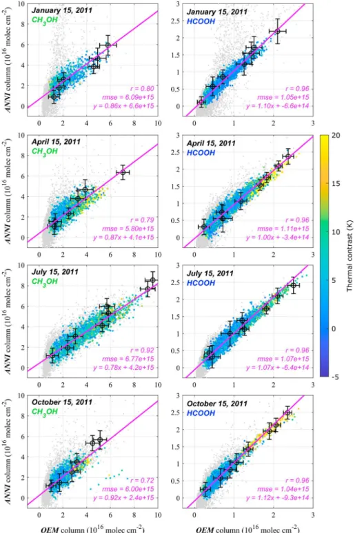
In this section, we compare the NN-derived gas columns with those obtained from a retrieval relying on the optimal estimation method (OEM; Rodgers, 2000) and performed with Atmosphit. This comparison is not only useful for assessing the NN retrieval; it also provides insights into the respective strengths and weaknesses of the two retrieval approaches. In addition, it allowed us to fix the calibration offsets for CH3OH and HCOOH presented in the previous section. The OEM retrieval requires a priori vertical profiles for each of the retrieved gases. For consistency, we used the same model-derived profiles as those used for the forward simulations (see section 3.1). Here we retrieved with Atmosphit a column scaling factor of the a priori to be consistent with the forward simulations which rely on the scaling of a fixed vertical gas profile. In view of the time required by line-by-line radiative transfer inversions, the OEM retrievals were performed only over a few selected days (15 January, April, July, and October 2011) and selected areas corresponding to source and remote regions (shown in Figure S5 in the supporting information). This consists of approximately 35,000 spectra. The main OEM retrieval parameters that were used are given in Table S1 in the supporting information.
In Figure 7, the OEM-retrieved columns of CH3OH and HCOOH over land are plotted against the
correspond-ing NN-derived columns, as a function of TC. The same figure, but for the retrievals over oceans, is provided in Figure S6 in the supporting information. The illustrated error bars (in black) for the OEM retrievals are the gas column corresponding to the total error (sum of the smoothing and measurement errors) on the retrieved col-umn scaling factor provided for each measurement by Atmosphit, while the error bars for the ANNI retrievals are the retrieved column uncertainty estimated on a per-pixel basis (see section 4.1). The NN-derived columns of the VOCs in Figure 7 have already been corrected for the column offset given in section 4.2. These offsets were determined from the mode of the differences between the two data sets. For the NN retrievals, the post-filters described in section 4.1 were applied. For the OEM retrievals, only columns with uncertainties lower than 60% were retained. The data that did not pass these quality flags is shown in Figures 7 and S6 (in the supporting information) in light gray.
The intercomparison plots reveal, for the three species, regression slopes mostly between 0.85 and 1.1 as well as high coefficients of correlation (r). This is especially the case for HCOOH for which the correlation coefficient is 0.96 for the four seasons and for which the regression slopes lie between 1 and 1.12. The retrieval consistency of CH3OH is also very good with regression slopes of 0.78–0.92 and correlation coefficients between 0.79 and 0.92. The agreement with summertime retrievals is unsurprisingly the best, as the sensitivity is higher in that period. The dynamic range of the CH3OH retrievals is a bit lower than for HCOOH, which could explain the slightly lower correlation coefficients. However, given the challenging retrieval in the spectral range largely dominated by O3, the consistency of the CH3OH retrievals can also be considered very satisfactory.
The comparison for PAN exhibits much larger scatter than for the other two species (r = 0.72 in the summer, see Figure S7 in the supporting information). This is likely linked to the difficulty of the radiative transfer code to reproduce the observed baseline over a wide spectral range (due to, e.g., broadband-interfering species and variable surface emissivity), which is critical for this compound characterized by broadband absorption features. The large scatter also prevents an accurate estimation of the offset, which is the reason why we relied for this on a model (see section 4.2).
The comparisons for CH3OH and HCOOH demonstrate the ability of the NN to retrieve reliable gas columns
Journal of Geophysical Research: Atmospheres
10.1029/2018JD029633
Figure 7. Comparison between CH3OH and HCOOH total columns from the ANNI processing (yaxis) and retrieved with an OEM (xaxis). Pixels are colored by thermal contrast. The spectra have been selected from 4 days of 2011 over specific regions (see Figure S5). Postfiltering has been applied to both data sets (see section 4.1). The measurements filtered out of the comparison are depicted as gray dots. The linear regression, root-mean-square error (rmse) and coefficient of correlation (r) between the two data sets are given in magenta. The ANNI and OEM uncertainties for random measurements are also indicated for selected measurements (in black). The present comparison only includes
measurements performed over land. Figure S6 illustrates the same comparison for the observations over oceans. ANNI = Artificial Neural Network for IASI; IASI = Infrared Atmospheric Sounding Interferometer; OEM = optimal estimation method.
does not allow deciding which retrieval provides the most accurate results. Indeed, while the NN retrieval should theoretically have the largest sensitivity to the target trace gas through its dependence on the HRI (see, e.g., Clarisse et al., 2013; Walker et al., 2011; Whitburn et al., 2016), it might suffer from biases in the HRI or the NN itself. The OEM retrieval, which tries to reconstruct the IASI spectrum in a spectral range of interest, is sensitive to the degree to which the interfering species are realistically adjusted. As an example, the relia-bility of the OEM retrieval of CH3OH will depend primarily on the fit of O3. In addition, OEM retrievals can be
significantly affected by the choice of a priori constraints. Both approaches differ most when the sensitivity to the target gas is low (gray dots in Figures 7 and S6). For such observations, the OEM retrievals are significantly biased toward the a priori, whereas the NN retrievals are more noisy but theoretically unbiased.
5. ANNI Products and Global Distribution Overview
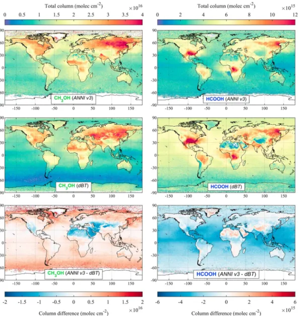
5.1. Comparison with Previous Products
Global distributions of CH3OH and HCOOH have already been produced from IASI observations, using dBT-based approaches (Pommier et al., 2016; Razavi et al., 2011). In this section, we compare the new retrievals with the former products. For this purpose, we have reproduced for 2011 the CH3OH and HCOOH global distributions following the approaches described by Razavi et al. (2011) and Pommier et al. (2016), respec-tively. Figure 8 presents the ANNI- and dBT-derived distributions over Northern Hemisphere summer in 2011, and the absolute difference between the averaged ANNI-columns and the dBT-columns. The same compari-son, but for the boreal winter, is shown in Figure S8 in the supporting information. Overall, the two retrieval approaches produce consistent distributions for CH3OH and HCOOH, with respect to the main source regions
and transport patterns (see sections 5.2 and 5.3). The new ANNI-CH3OH are on average ∼0.5 × 10¹⁶molec/cm2
higher than the corresponding dBT-derived columns (in both summer and wintertime). In the summer over the oceans at high latitude, the differences can reach ∼1 × 10¹⁶molec/cm2. Depending on the season, both
products significantly differ over deserts, but it is worth mentioning that these areas were mainly filtered out in the final dBT-product (Razavi et al., 2011). The largest differences between the two HCOOH data sets are found over the oceans, where the ANNI product is significantly lower (up to 2 × 10¹⁵molec/cm2between the
Tropics) in both boreal summer and winter. This difference could be linked to the dependence of the HCOOH spectral signature on the atmospheric H2O column, which is fully taken into account in ANNI, whereas only a
first-order H2O correction was performed by Pommier et al. (2016). Over land, the ANNI product is also slightly
lower, with ANNI-dBT column differences typically ranging between −2 and 0.5 × 10¹⁵molec/cm2. Pommier
et al. (2016) reported an overall high bias of the dBT-based HCOOH product compared to ground-based Fourier Transform Infrared (FTIR) measurements. Given that the retrieved ANNI columns are lower, it can be expected that comparison with independent measurements will show an improved agreement.
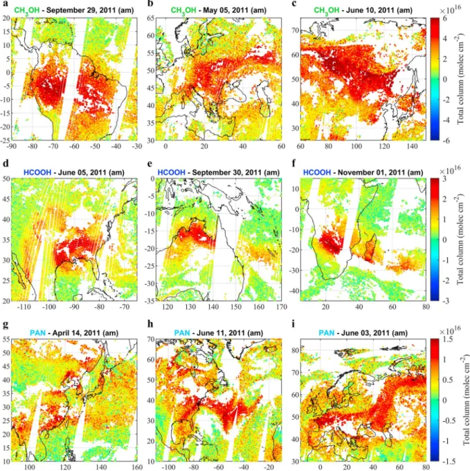
5.2. Single Overpass Examples
To illustrate the new ANNI products, the distributions of CH3OH, HCOOH, and PAN columns derived from the morning IASI overpasses on 1 day of 2011 and over specific regions are presented in Figure 9. In this figure, each colored dot corresponds to an individual IASI measurement. The empty spaces are due to the gap between successive satellite orbits (within the Tropics, mainly), cloudy scenes (prefiltering) and column data discarded after the retrieval process (postfiltering). Examples were chosen over source regions or to illustrate large transport patterns:
• Large columns of CH3OH (up to over 5 × 10¹⁶molec/cm2) are retrieved daily from the IASI measurements
over, e.g., the Amazonian forest in September (Figure 9a)—which also corresponds to the period of large biogenic VOC emissions from the tropical forests (e.g., Guenther et al., 1995, 2006)—as well as over central Europe (Figure 9b) and from the boreal forests of Siberia (Figure 9c) during the Northern Hemisphere spring and summer, respectively. This is consistent with our general knowledge on CH3OH, which is primarily an emitted compound of biogenic origin (e.g., Duncan et al., 2007; Millet et al., 2008; Singh et al., 1995, 2001; Stavrakou et al., 2011; Tie et al., 2003; Wells et al., 2014).
• The global sources of HCOOH are not well known and the global consensus is that its emissions are signifi-cantly underestimated. However, it is admitted that most of the HCOOH sources are secondary and related to a large suite of precursors, mainly of biogenic origin (e.g., Millet et al., 2015; Stavrakou et al., 2012). Hot spots of HCOOH with total columns over 2 × 10¹⁶molec/cm2are indeed observable in isoprene-dominated
environments, like over the Southeast United States in June (Figure 9d) and northern Australia in September (Figure 9e). Other hot spots are found in biomass burning regions, as, for instance, in the southern parts of Africa during the fire season (Figure 9f; e.g., Chaliyakunnel et al., 2016). Figure 9f illustrates well, with large
Journal of Geophysical Research: Atmospheres
10.1029/2018JD029633
Figure 8. Comparison between the ANNI-CH3OH and ANNI-HCOOH products, and the global distributions obtained from IASI with retrieval methods based on dBT (Razavi et al., 2011, for CH3OH and Pommier et al., 2016, for HCOOH), over the boreal summer (June–August) of the year 2011. The comparison for the boreal winter (December–February) is shown in Figure S8 in the supporting information.
plumes of HCOOH originating from these hot spots, that IASI allows monitoring the transport of HCOOH and indirectly of its long-lived precursors.
• PAN formation is conditioned by the presence of oxygenated VOC precursors and NOx(e.g., Fischer et al., 2014, 2011). In such “polluted” environments like eastern Asia, eastern United States and western Europe, large PAN columns (over 1 × 10¹⁶molec/cm2) are indeed retrieved with the ANNI-PAN product. PAN being
relatively stable at cold temperature in the free troposphere, it is subject to long distance transport from source to remote regions following the dominant atmospheric circulation pattern. This is highlighted in Figures 9g–9i with plumes detected by IASI over the North Pacific Ocean, the North Atlantic Ocean, and Europe.
5.3. Global Distributions
Figures 10–12 present the seasonal near-global distributions of CH3OH, HCOOH, and PAN total columns for
the year 2011. The distributions are averages on a 0.5 × 0.5∘ grid of the individual measurements from the IASI morning overpasses. The distributions made with the p.m. IASI measurements (evening orbits) are shown in the supporting information (Figures S9–S11).
Figure 9. CH3OH, HCOOH, and PAN total column distributions retrieved over areas of interest with the ANNI method from 1 day of a.m. (morning overpasses) IASI observations. Each colored dot corresponds to an individual IASI measurement. The blank spaces are due to gaps between the successive satellite orbits (within the Tropics) or to data filtered out because of clouds or postfiltering (bad retrievals). ANNI = Artificial Neural Network for IASI; IASI = Infrared Atmospheric Sounding Interferometer; PAN = peroxyacetyl nitrate.
The global distributions of CH3OH, HCOOH, and PAN is consistent with our knowledge of these species and of
atmospheric chemistry in general, that is, CH3OH is directly emitted into the atmosphere from plant growth
mainly, whereas HCOOH and PAN are secondary products from a suite of biogenic, anthropogenic, and pyro-genic precursors whose degradation is enhanced by temperature and sunlight. The distributions highlight, in particular, the important contribution of biogenic emissions from the tropical forests (Amazonia, cen-tral Africa, and north Auscen-tralia) to the gas abundance. The IASI data reveals large enhancements of CH3OH, HCOOH, and PAN columns throughout the year over tropical regions and during summer at middle and high latitudes, which can be attributed to large primary emissions of CH3OH and of biogenic precursors of HCOOH and PAN. The VOC tropical emissions appear to be largest in September–November, which corresponds to the peak of the biomass burning season in South America and Africa. Clear transport patterns are found over the oceans in tropical regions, which is consistent with the relatively long tropospheric lifetime of the three species (typically over 10 days). In the Northern Hemisphere, the atmospheric abundance of CH3OH, HCOOH,
Journal of Geophysical Research: Atmospheres
10.1029/2018JD029633
Figure 10. Seasonal means (on a 0.5×0.5∘grid) of the ANNI-CH3OH total columns from the a.m. (morning overpasses) IASI measurements over the year 2011. The same distributions, but produced from the p.m. (evening overpasses) IASI observations, are shown in Figure S9 in the supporting information. ANNI = Artificial Neural Network for IASI; IASI = Infrared Atmospheric Sounding Interferometer.
and PAN exhibits a pronounced seasonal cycle: the total columns are low during the boreal winter, increase in spring and eventually peak during the boreal summer. This seasonal cycle is mainly driven by meteorol-ogy and its impact on vegetation growth, with important source contributions from the boreal forests as well as from the Southeast United States. Emissions from India, Southeast Asia, and China also contribute with anthropogenic emissions of PAN precursors throughout the year. The transport patterns of CH3OH, HCOOH,
and PAN observed over the oceans can be traced back to the continental emissions.
Rather sharp ocean-land discontinuities can be observed in the seasonal means, especially for PAN at high lat-itudes. These likely stem from the use of fixed emission and transport profiles. To gain a better understanding of the impact of these on the retrieval, a sensitivity test was performed on 1 day of spectra. For each target species and for all the IASI observations, the NNs trained with the emission and the transport gas vertical profile were used in turn to retrieve the gas columns, yielding two separate estimates of the true column. Dif-ferences were found to be around 20% for CH3OH and HCOOH, and around 30% for PAN (see Figure S12 in the
supporting information). These differences largely explain the observed transition between land and ocean columns.
The distributions of CH3OH, HCOOH, and PAN derived from the p.m. observations (Figures S9–S11) are similar to the a.m.-derived distributions (Figures 10–12). The IASI measurements from the evening satellite over-passes are characterized by overall weaker TC than those from the morning overover-passes. This weaker TC translates to a weaker sensitivity of the IASI measurement to the lower tropospheric layers, which leads to generally smaller HRI values for constant trace gas abundances. As long as this sensitivity exceeds a minimum threshold, the NN is able to take into account this effect, and so no large a.m. to p.m. differences are expected given the longevity of these species. However, differences are found for CH3OH and especially for HCOOH
over emission regions (e.g., tropical and boreal forests). One likely reason stems from the postfiltering, which removes more data from the evening overpass and can lead to biases in the seasonal averages. Another rea-son might be the use of constant vertical profiles. As explained above, the NN can account for changes in thermal contrast. However, the HRI-to-column conversion will only be consistent for varying thermal contrast if the vertical profile used in the retrieval corresponds to the actual profile. As the largest a.m. to p.m. dif-ferences are found over emission regions, this suggest that the modeled profiles used to set up the training
Figure 11. Seasonal means (on a 0.5×0.5∘grid) of the ANNI-HCOOH total columns from the a.m. (morning overpasses) IASI measurements over the year 2011. The same distributions, but produced from the p.m. (evening overpasses) IASI observations, are shown in Figure S10 in the supporting information. ANNI = Artificial Neural Network for IASI; IASI = Infrared Atmospheric Sounding Interferometer.
database might not be fully representative of the true profiles over such environments. Finally, possible diurnal variability in the emissions of CH3OH, HCOOH, and PAN and/or of their precursors may also be at play. In contrast to HCOOH and CH3OH, the PAN column distributions obtained with the p.m. IASI observations
(Figure S11) match almost perfectly those of the morning overpasses (Figure 12). This is likely because PAN retrieval is less affected by variations in the TC as its concentrations in the lower troposphere are proportionally lower than those of the other species.
6. Conclusion and Outlooks
Initially developed for the retrieval of NH3, the ANNI retrieval approach has been generalized to allow the
derivation of vertical columns of several VOCs (CH3OH, HCOOH, and PAN) from the IASI spectra. Incremental improvements in all steps of the retrieval procedure have been introduced.
The four main advantages of the ANNI retrieval approach over more traditional physical retrieval approaches are (see also section 7 in Whitburn et al., 2016 for a more comprehensive discussion):
• Because of its reliance on HRI, the retrieval can exploit efficiently large spectral ranges and provides a close to optimal sensitivity to the trace gas.
• Not relying on a priori information, the products are in principle suitable to be averaged at face value to produce unbiased averages.
• The forward model is less important than for retrievals relying on spectral fitting (as was illustrated here with the problems encountered for PAN).
• The retrieval is computationally very efficient. This not only allows the processing of global IASI data over large periods but also allows for shorter development cycles.
Despite the many advantages, the ANNI retrieval method also has its drawbacks:
• Using fixed vertical gas profiles can be a limitation. In general, IASI spectra contain practically no information on the vertical distribution for weak infrared absorbers such as NH3or the VOCs. However, in favorable cases,
Journal of Geophysical Research: Atmospheres
10.1029/2018JD029633
Figure 12. Seasonal means (on a 0.5×0.5∘grid) of the ANNI-PAN total columns from the a.m. (morning overpasses) IASI measurements over the year 2011. The same distributions, but produced from the p.m. (evening overpasses) IASI observations, are shown in Figure S11 in the supporting information. ANNI = Artificial Neural Network for IASI; IASI = Infrared Atmospheric Sounding Interferometer; PAN = peroxyacetyl nitrate.
exhibiting emission lines (Bauduin et al., 2017) as such lines can only originate from atmospheric layers associated with negative thermal contrast.
• While ANNI does not rely on a priori information on the total column, it also does not produce averaging kernels, which characterize the measurement sensitivity and which are useful in the assimilation of the data with models and for validation with vertically resolved profiles. The uncertainty estimate associated with the ANNI retrieval only partially provides such information.
The seasonal averages, the intercomparison of the new products with an OEM retrieval, and comparison with previously derived products give confidence in the reliability of the newly derived CH3OH, HCOOH, and PAN
products. Forthcoming work will be dedicated to the formal validation of the retrieved columns via com-parison with independent measurements, for example, from ground-based FTIR spectroscopy and aircraft campaigns.
Illustrations of the new products were provided here with measurements of a single year of IASI operation (2011). These examples highlight the advantage of the daily high sampling of IASI, as well as the poten-tial of the ANNI products for tackling scientific questions related to atmospheric gas sources, transport and chemistry. Taking full advantage of the computing efficiency of the NN-based approach, the retrievals have also been applied to the whole time series of IASI observations, which starts in 2007 with IASI on board the Metop-A platform and also includes IASI/Metop-B since 2012. As a result, over 10 years—and still ongoing—of global distributions of CH3OH, HCOOH, and PAN total columns are now available. Moreover, with
the recent launch of IASI/Metop-C (November 2018) and the future IASI-NG (New Generation) instruments on board the three Metop-SG-A platforms (first launch planned for 2021), at least another 25 years are foreseen. Altogether, this suite of CH3OH, HCOOH, and PAN observations from a single satellite sounder is unique.
While the comparison with the optimal estimation retrievals already gives a high degree of confidence in the retrieved products, especially for PAN, a formal validation with independent measurements is needed. Beyond the overview given here, further analysis of the retrieved distributions will give precious insights into the source regions and types of the investigated species, as well as into their transport, seasonality, and interannual variability. One limitation, which is present for all the satellite-derived products of minor trace