HAL Id: insu-01405271
https://hal-insu.archives-ouvertes.fr/insu-01405271
Submitted on 29 Nov 2016
HAL is a multi-disciplinary open access
archive for the deposit and dissemination of
sci-entific research documents, whether they are
pub-lished or not. The documents may come from
teaching and research institutions in France or
abroad, or from public or private research centers.
L’archive ouverte pluridisciplinaire HAL, est
destinée au dépôt et à la diffusion de documents
scientifiques de niveau recherche, publiés ou non,
émanant des établissements d’enseignement et de
recherche français ou étrangers, des laboratoires
publics ou privés.
The Swarm Initial Field Model for the 2014 geomagnetic
field
Nils Olsen, Gauthier Hulot, Vincent Lesur, Christopher Finlay, Ciaran
Beggan, Arnaud Chulliat, Terence Sabaka, Rune Floberghagen, Eigil
Friis-Christensen, Roger Haagmans, et al.
To cite this version:
Nils Olsen, Gauthier Hulot, Vincent Lesur, Christopher Finlay, Ciaran Beggan, et al.. The Swarm
Ini-tial Field Model for the 2014 geomagnetic field. Geophysical Research Letters, American Geophysical
Union, 2015, 42 (4), pp.1092-1098. �10.1002/2014GL062659�. �insu-01405271�
RESEARCH LETTER
10.1002/2014GL062659Special Section:
ESA’s Swarm Mission, One Year in Space
Key Points:
• First geomagnetic model from Swarm satellite constellation data • Magnetic gradient data enhance the
spatial resolution of geomagnetic models
Correspondence to:
N. Olsen, [email protected]
Citation:
Olsen N., et al. (2015), The Swarm Initial Field Model for the 2014 geomagnetic field, Geophys.
Res. Lett., 42, 1092–1098,
doi:10.1002/2014GL062659.
Received 29 NOV 2014 Accepted 30 JAN 2015
Accepted article online 3 FEB 2015 Published online 25 FEB 2015
The Swarm Initial Field Model for the 2014
geomagnetic field
Nils Olsen1, Gauthier Hulot2, Vincent Lesur3, Christopher C. Finlay1, Ciaran Beggan4,
Arnaud Chulliat5, Terence J. Sabaka6, Rune Floberghagen7, Eigil Friis-Christensen1,
Roger Haagmans8, Stavros Kotsiaros1, Hermann Lühr3,
Lars Tøffner-Clausen1, and Pierre Vigneron2
1DTU Space, National Space Institute, Technical University of Denmark, Kongens Lyngby, Denmark,2Equipe de
Géomagnétisme, Institut de Physique du Globe de Paris, Sorbonne Paris Cité, Université Paris Diderot, UMR 7154 CNRS/INSU, Paris, France,3Helmholtz-Zentrum Potsdam, Deutsches GeoForschungsZentrum, Potsdam, Germany,4British
Geological Survey, Edinburgh, UK,5National Geophysical Data Center, NOAA, Boulder, Colorado, USA,6Planetary
Geodynamics Branch, NASA GSFC, Greenbelt, Maryland, USA,7Directorate of Earth Observation Programmes, ESRIN, Frascati, Italy,8ESA/ESTEC, Noordwijk, Netherlands
Abstract
Data from the first year of ESA’s Swarm constellation mission are used to derive the Swarm Initial Field Model (SIFM), a new model of the Earth’s magnetic field and its time variation. In addition to the conventional magnetic field observations provided by each of the three Swarm satellites, explicit advantage is taken of the constellation aspect by including east-west magnetic intensity gradient information from the lower satellite pair. Along-track differences in magnetic intensity provide further information concerning the north-south gradient. The SIFM static field shows excellent agreement (up to at least degree 60) with recent field models derived from CHAMP data, providing an initial validation of the quality of the Swarm magnetic measurements. Use of gradient data improves the determination of both the static field and its secular variation, with the mean misfit for east-west intensity differences between the lower satellite pair being only 0.12 nT.1. Introduction
The three-satellite constellation mission Swarm was launched by the European Space Agency (ESA) on 22 November 2013. Swarm consists of three identical spacecraft, two of which (Swarm Alpha, in following denoted as SW-A, and Swarm Charlie, SW-C) are flying almost side by side in polar orbits (of inclination 87.4◦) at lower altitude (about 465 km above a mean radius of a = 6371.2 km in January 2015). The east-west separation of their orbits is 1.4◦in longitude corresponding to 155 km at the equator. The third satellite,
Swarm Bravo (SW-B) is in a slightly higher (about 520 km altitude in January 2015) orbit of inclination 88◦. Each of the three satellites carries an Absolute Scalar Magnetometer (ASM) for measuring Earth’s magnetic field intensity, a Vector Fluxgate Magnetometer (VFM) measuring the direction and strength of the magnetic field, and a three-head Star Tracker mounted close to the VFM to obtain the attitude needed to transform the vector readings to a known coordinate frame. Time and position are provided by onboard GPS. The payload also includes instruments to measure plasma and electric field parameters as well as gravitational acceleration. More information about the mission after 1 year in space can be found in R. Floberghagen et al. (The Swarm mission—An overview one year after launch, submitted to Earth, Planets
and Space, 2015). All Swarm data are available at http://earth.esa.int/swarm.
This paper describes a model of the Earth’s magnetic field that has been derived from the first year of Swarm magnetic data. For this model we use observations of the magnetic field intensity and direction as well as information on the horizontal gradient of the magnetic field. Approximations of the north-south (N-S) gradient are obtained from along-track differences of intensity measurements at each of the three satellites following an approach that has recently been applied to data from the CHAMP satellite [Kotsiaros et al., 2015;
Sabaka et al., 2015]. In addition, and for the first time in geomagnetic field modeling, we also use estimates
of the east-west (E-W) field gradient by taking the difference of the magnetic field intensity measured by the lower Swarm satellite pair, SW-A and SW-C.
Geophysical Research Letters
10.1002/2014GL062659
Jan 14 Apr 14 Jul 14 Oct 14 Jan 15 0 2 4 6 8 10 12 time
total number of data points
per 10 day bin
−90 −60 −30 0 30 60 90 0 2 4 6 8 10 12 x 104 x 104 QD latitude [°]
total number of data points
per 5° latitude bin
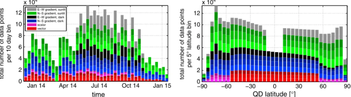
Figure 1. Total number of Swarm satellite data (stacked histogram) as a function of (left) time and (right) latitude, respectively. For vector (red), scalar (purple), and N-S gradient (blue and green) data, the dark/normal/light color represents SW-A/SW-B/SW-C. E-W gradient data are shown in black and grey.
2. Data Selection and Model Parameterization
We used nearly 14 months (26 November 2013 to 17 January 2015) of magnetic data from the three Swarm satellites. Nightside data during geomagnetically quiet times, downsampled to 30 s by taking one data point in 30 from the 1 Hz Level 1b-data (version 0302 when available, otherwise version 0301), have been selected using the same criteria as for the CHAOS-4 model [Olsen et al., 2014]. In particular, we select data (vector and scalar) from dark regions only (Sun at least 10◦below the horizon) for which the strength of the magnetospheric ring-current, estimated using the RC index [Olsen et al., 2014], changed by at most 2 nT/h. At quasi-dipole (QD) latitudes [Richmond, 1995] equatorward of ±55◦, we require that the geomagnetic activity index Kp ≤ 2◦, while for regions poleward of 55◦QD latitude the weighted average over the preceding 1 h of the merging electric field at the magnetopause [e.g., Kan and Lee, 1979; Newell et al., 2007] has to be below 0.8 mV/m.
Three vector components of the magnetic field were taken for nonpolar latitudes (equatorward of ±55◦QD latitude), while only scalar data were used for higher latitudes. Each vector measurement of the VFM BVFM has been normalized such that its intensity is equal to that measured by the ASM:|BVFM| = FASM.
In addition to these data of the magnetic field, we include horizontal difference data (“gradient data”) of magnetic intensity F. In contrast to the selection of magnetic vector and scalar field data (Kp≤ 20,
|dRC∕dt| < 2 nT/h, a condition that is fulfilled for 27% of the time), we allow for higher geomagnetic activity when selecting gradient data (Kp< 30, |dRC∕dt| < 3 nT/h, which is fulfilled for 45% of the time) and also
use gradient data from the dayside. We choose to exclude dayside data at QD latitudes< ± 10◦to avoid contamination by the equatorial electrojet.
In order to approximate the east-west gradient, we took the difference of scalar intensity data,
𝛿FEW= ±[FA(t1, r1, 𝜃1, 𝜙1) − FC(t2, r2, 𝜃2, 𝜙2)], measured by the two satellites SW-A and SW-C. Here
ti, ri, 𝜃i, 𝜙i, i = 1–2 are time, radius, geographic colatitude, and longitude of the two observations. The sign of
the difference was chosen such that𝛿𝜙 = 𝜙1−𝜙2> 0. We do not divide the field differences by the spatial distance between the observations to obtain a spatial gradient with units nT/km, because we prefer to work with magnetic field differences with units nanotesla. For each scalar observation FA(from SW-A) fulfilling the
above selection criteria, we selected the corresponding value FC(from SW-C) that was closest in colatitude 𝜃, with the additional requirement that |𝛿t| = |t1− t2| < 50 s.
The north-south gradient is approximated by the difference𝛿FNS= ±[Fk(tk, rk, 𝜃k, 𝜙k) − Fk(tk+ 15 s, rk+𝛿r, 𝜃k+𝛿𝜃, 𝜙k+𝛿𝜙)] of subsequent scalar data measured by the same satellite (k = 1, 2, or 3) 15 s later,
corresponding to an along-track distance of ≈115 km (≈1◦in latitude near the equator). The sign of the difference was chosen positive if𝛿𝜃 > 0, otherwise negative. We have only used scalar gradient data since the treatment of vector gradient data is much more demanding, in particular due to the “VFM-ASM disturbance field” that is presently under investigation.
Histograms of the data distribution in time and latitude are presented in Figure 1. E-W gradient data (shown in black/grey) are not available before April 2014 because the two satellites SW-A and SW-C have been flying in their nominal constellation (side by side) only since 18 April 2014. Exclusion of dayside near-equatorial gradient data is the reason for the decrease in the number of data at<±10◦QD latitude.
All data are weighted proportional to sin𝜃 to simulate an equal-area distribution. Anisotropic magnetic errors due to attitude uncertainty [e.g., Holme and Bloxham, 1996] are considered assuming an error in the scalar intensity of𝜎F= 2 nT and an isotropic attitude error of 5 arcsec. The value of𝜎F= 2 nT is considerably
higher than the measurement uncertainty of ≈ 0.2 nT because it also includes errors introduced by unmodeled magnetic field sources, mainly of external origin. However, since these external fields are rather large scale and cancel out when taking differences of nearby measurements, we are able to adopt an a priori data error of𝜎𝛿F= 0.2 nT for the magnetic field differences (i.e., the gradient data).
The model parameterization follows closely that of CHAOS-4. It consists of spherical harmonic expansion coefficients describing the magnetic field vector in an Earth-Centered Earth-Fixed (ECEF) coordinate system and sets of Euler angles needed to rotate the satellite vector readings from the magnetometer frame to the star tracker frame. The magnetic field vector in the ECEF frame, B = −∇V, is derived from a magnetic scalar potential V = Vint+ Vextconsisting of a part, Vint, describing internal (core and lithospheric) sources, and a
part, Vext, describing external (mainly magnetospheric) sources and their Earth-induced counterparts. Both
parts are expanded in terms of spherical harmonics. For the internal part this yields
Vint= a Nint ∑ n=1 n ∑ m=0 ( gmncos m𝜙 + hmn sin m𝜙) ( a r )n+1 Pmn (cos𝜃) (1)
where (r, 𝜃, 𝜙) are geographic coordinates, Pm
n are the associated Schmidt seminormalized Legendre
functions,{gm n, h
m n
}
are the Gauss coefficients describing internal sources, and Nint = 70 is the maximum
degree and order of the internal expansion. Coefficients up to degree n = 13 include a linear dependence on time (linear secular variation). This yields 70 × 72 + 13 × 15 = 5235 coefficients describing the internal part of Earth’s magnetic field.
The external part of the field model is identical to that of CHAOS-4, with an expansion of the near magnetospheric sources (magnetospheric ring current) in the Solar Magnetic (SM) coordinate system (up to
n = 2, with special treatment of the n = 1 terms) and of remote magnetospheric sources (e.g., magnetotail
and magnetopause currents) in Geocentric Solar Magnetospheric coordinates (also up to n = 2 but restricted to order m = 0). We solve for an RC baseline correction (described by SM dipole coefficients that explicitly vary in time) in bins of 5 days (for m = 0) and 30 days (for m = 1), respectively, which in total results in 118 parameters describing the external field part of the model. See section 3 of Olsen et al. [2014] for details. As part of the model estimation we solve for the Euler angles describing the rotation between the vector magnetometer frame and the star tracker frame in bins of 10 days (i.e., 3 × 41, 40 and 35 sets of angles for satellites Alpha, Bravo, and Charlie, respectively, resulting in an additional 348 model parameters). The 5701 model parameters are estimated from approximately 4 × 10⁶observations (105,775 scalar data,
3× 394,218 = 1,182,654 vector data, and 2,680,668 estimates of scalar gradients) by means of a regularized
Iteratively Reweighted Least Squares approach using Huber weights. The gradient data were handled in a
manner similar to that described in Kotsiaros et al. [2015] by taking the difference of the design matrices corresponding to the two positions ti, ri, 𝜃i, 𝜙i, i = 1–2. Gradient dayside data do not contribute to the core
field part of the model (i.e., internal Gauss coefficients up to n = 13), whereas the remaining parts of the model are constrained by all data. No model regularization has been applied.
3. Results and Discussion
Table 1 lists the number of data points, together with means and root-mean-squared (RMS) misfit values between the observations and the predictions of the Swarm Initial Field Model (SIFM) model. At nonpolar latitudes the RMS misfit to the radial component Bris below 2 nT, demonstrating the excellent quality of
the Swarm magnetic field data. The RMS misfit of scalar intensity F and of the horizontal components is slightly higher, probably due to the impact of remaining unmodeled contributions from magnetospheric currents. Even more remarkable is the RMS misfit of the gradient data which (for dark conditions) is below 0.2 nT for the N-S gradient (obtained using data from the same instrument) and below 0.3 nT when looking at the difference between SW-A and SW-C. The nonzero mean value of −0.12 nT for the nonpolar, dark 𝛿FEW
Geophysical Research Letters
10.1002/2014GL062659
Table 1. NumberNof Data Points, (Huber-Weighted) Mean, and RMS Misfit (in nT) of Scalar (F), Vector (Br, B𝜃, B𝜙), N-S Gradient (𝛿FNS), and E-W Gradient (𝛿FEW) Data, at Polar (> ±55◦) and Nonpolar (< ±55◦) QD Latitudes
SW-A SW-B SW-C SW-A – SW-C
N Mean RMS N Mean RMS N Mean RMS N Mean RMS
Fpolar 35,606 −0.27 3.47 36,387 −0.15 3.45 33,782 −0.13 3.45 Fnonpolar 137,164 0.04 2.49 136,259 0.02 2.48 120,795 0.06 2.51 Br 137,164 0.00 1.97 136,259 −0.02 2.04 120,795 0.04 1.95 B𝜃 137,164 −0.13 3.23 136,259 −0.12 3.33 120,795 −0.20 3.31 B𝜙 137,164 −0.03 2.52 136,259 −0.05 2.52 120,795 −0.03 2.48 𝛿FNS,polar 285,484 −0.01 1.12 287,940 −0.01 1.05 236,417 −0.02 1.06 𝛿FNS,nonpolar,dark 198,626 0.00 0.19 198,955 0.00 0.18 167,801 0.00 0.18 𝛿FNS,nonpolar,sunlit 217,910 0.02 0.34 219,557 0.02 0.32 176,916 0.01 0.33 𝛿FEW,polar 279,777 −0.12 0.54 𝛿FEW,nonpolar,dark 197,769 −0.12 0.28 𝛿FEW,nonpolar,sunlit 211,152 −0.03 0.44
instrumental error budget of 0.3 nT. The dayside RMS misfits are slightly higher due to enhanced ionospheric contributions.
Figure 2a shows Mauersberger-Lowes spectra of the static (lithospheric) field part of the SIFM model and of analogous models derived from various data subsets: SIFMno gradient, which was derived from vector and
scalar intensity data without including gradient data; SIFMNS gradient, which also included N-S gradient but
no E-W gradient data; and SIFMEW gradient, similar but including E-W gradient and no N-S gradient data. For
reference we also present spectra from the MF7 [Maus, 2010] and CHAOS-4 [Olsen et al., 2014] lithospheric field models, both derived mainly from CHAMP satellite data and not using any Swarm data.
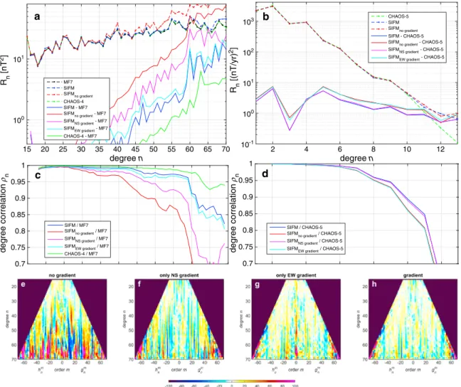
Excluding gradient data (model SIFMno gradient) leads to a lithospheric field model very similar to that of MF7 and CHAOS-4 up to degree n = 40, but with considerably more power above that degree (see dashed red curve). Including gradient data to build model SIFM reduces this power, making this model likely reliable up to at least n = 60 (see blue-dashed curve). This is also confirmed by the degree correlation of the various intermediate SIFM models with respect to MF7 (shown in Figure 2c). Note in particular the crucial improvement brought by the inclusion of the innovative E-W gradient data.
Figures 2e–2h present the relative difference between each coefficient of the different SIFM versions and MF7 in a degree versus order matrix and show that it is primarily high-degree coefficients that are modified when gradient data are included. A model built only from field data shows significant differences with respect to MF7 (Figure 2e), whereas inclusion of gradient data results in much better agreement (Figure 2h). In particular, N-S gradient data improve the determination of high-degree near-zonal coefficients (|m|≈0≪n), while E-W gradient data improve the near-sectorial terms (|m|≈n≫0). There are, however, systematic differences between SIFM and MF7 in the sectorial terms above n = 45. This is likely due to a Backus effect [e.g., Backus, 1970; Stern and Bredekamp, 1975]. High-degree lithospheric field coefficients (above n = 45 or so) are primarily constrained by scalar gradient data, but these do not provide information concerning the small-scale details of the location of the dip equator, which is necessary to avoid this effect [Khokhlov et al., 1997; Ultré-Guérard et al., 1998]. This mainly affects the tesseral coefficients gn
n, h n
nand leads
to models that are erroneous near the dip equator. Indeed, when looking at the difference in Brbetween
SIFM and MF7 the largest deviations occur in that region (Figure 3, right). In spite of this, the agreement between the two models is noteworthy, with an RMS vector field difference of only 7.5 nT (reduced to 6.9 nT when excluding QD latitudes<±10◦). Inclusion of more vector data will certainly help to reduce the Backus effect.
In addition to the static field, the secular variation (SV) also benefits from the inclusion of gradient information. This is apparent from comparisons of the SV (for epoch 2014.5) predicted by the SIFM and the CHAOS-5 model (C. C. Finlay et al., DTU candidate field models for IGRF-12 and the CHAOS-5 geomagnetic field model, submitted to Earth, Planets and Space, 2015) which was derived from a combination of Ørsted, CHAMP, SAC-C, Swarm, and ground observatory data (Figure 2b). Some care is needed with this comparison,
degree n 15 20 25 30 35 40 45 50 55 60 65 70 Rn [nT 2] 100 101
a
degree n 2 4 6 8 10 12 Rn [(nT/yr) 2] 10-1 100 101 102 103b
0.7 0.75 0.8 0.85 0.9 0.95 1c
0.7 0.75 0.8 0.85 0.9 0.95 1d
Figure 2. Lowes-Mauersberger power spectra (a) of the static field (n = 15 − 70) and (b) of the linear SV (n = 1 − 13) from the SIFM together with various reference and data subset model at the Earth’s surface. Spectra of models are shown in dotted lines, spectra of differences between models in solid lines. Degree correlations of the SIFM and other models (c) with respect to model MF7 for the static field and (d) with respect to CHAOS-5 for the SV. Normalized coefficient differences (in %) with respect to MF7, for (e) SIFMno gradient, (f ) SIFMNSgradient, (g) SIFMEWgradient, and (h) SIFM, respectively.
Figure 3. (left) November 2013 to January 2015 rate of change ofBrat the CMB from SIFM for degreesn = 1 − 11. (right) Difference ofBrat Earth’s surface between SIFM and MF7, for degreesn = 16 − 65. Red lines locate the dip equator
Geophysical Research Letters
10.1002/2014GL062659
Figure 4. Residuals of the scalar (green) and scalar gradient (blue for N-S and red for E-W) data versus QD latitude for dark regions and magnetically quiet conditions. Note the nonlinearyaxis (∝ arctan(y∕5 nT)), which emphasizes near-zero values. Solid curves show the (Huber-weighted) mean value of the residuals in bins of2◦in latitude; dashed curves represent the mean±1 standard deviation.
since CHAOS-5 was derived using a temporal smoothing that increased with spherical harmonic degree, while the SIFM provides an estimate of the SV time-averaged over the year for which Swarm data are available. Nevertheless, the SIFM SV agrees better with the CHAOS-5 SV than does the SIFMnogradientSV. Interestingly,
this improvement arises mainly due to the inclusion of the N-S gradient data, which appear to be efficient at removing magnetospheric contamination of the zonal terms of the modeled SV. These results are extremely encouraging, as they show that Swarm is already able to resolve yearly snapshots of the SV up to approximately n = 11. Figure 3 (left) shows a map of the rate of change that occurred in Brbetween November 2013 and January 2015 at the
core-mantle boundary (CMB), as predicted from the SIFM SV up to n = 11.
The ability of gradient data to enhance the resolution of the SIFM is impressive. It is interesting, in this respect, to have a close inspection of residuals (data minus SIFM predictions) in the scalar data F, N-S scalar differences𝛿FNS, and E-W differences𝛿FEW, for dark regions and quiet conditions (Kp< 2, |dRC∕dt| ≤ 2 nT/h, Figure 4). As expected, the largest residuals occur in the auroral zone (QD latitudes between ±65◦and ±80◦) and are primarily a result of polar electrojet activity. In contrast, residuals within the polar cap (> ±85◦) and at nonpolar latitudes (< ±55◦) are generally much smaller. Residuals in F, on the other hand, display much larger RMS misfits even at nonpolar latitudes, ranging from 2 nT (near QD latitudes of ±35◦) up to 4 nT (near the dip equator). This is a clear signature of unmodeled contributions from the magnetospheric ring-current signal, which has a greater impact on F near the equator than at QD latitudes of ±35◦. This rapidly varying magnetospheric signal effectively behaves as a source of noise in F. Fortunately, it also is very large scale, and thus, it affects gradient data (based on quasi-synchronous data, recall section 2) much less. This is the reason that gradient data are able to help improve the quality of the field model, validating the gradient component of the Swarm constellation concept.
4. Conclusion and Perspectives
After 1 year in space, the Swarm mission has provided a wealth of valuable data. Despite calibration issues that currently limit a full use of the constellation configuration advantages (see R. Floberghagen et al., submitted manuscript, 2015), these data can already be used to produce extremely impressive results. The SIFM model presented here provides a clear illustration of what can already be achieved.
Perhaps most importantly, the SIFM model is able to provide a description of the static lithospheric field that is remarkably close to that of the MF7 [Maus, 2010] and CHAOS-4 [Olsen et al., 2014] models, up to at least degree and order 60, despite the fact that these earlier models did not use a single Swarm data and relied primarily on CHAMP data. This agreement provides both an initial validation of the Swarm mission and a valuable a posteriori validation of the CHAMP mission.
The SIFM model also provides an initial validation of the gradient concept underlying the Swarm mission [Friis-Christensen et al., 2006]. Although not yet capable of achieving what could possibly be achieved when including low-altitude data from later mission phases [Olsen et al., 2006], gradient data appear to be a very efficient way of increasing the resolution of geomagnetic field models.
More generally, the quality of the SIFM model is an encouraging preliminary result with regard to the core field and lithospheric field models [Rother et al., 2013; Sabaka et al., 2013; Thébault et al., 2013] to be built and distributed by ESA as so-called L2 products of the mission [see Olsen et al., 2013].
Finally, the demonstration that SV estimates up to n = 11 with a temporal resolution of 1 year can be built from Swarm data confirms that another important mission goal is within sight. The ability to study core field changes with high temporal resolution promises fresh insights on short-timescale core dynamics [see Finlay
et al., 2010], in particular regarding so-called geomagnetic jerks [Mandea et al., 2010], pulses [Chulliat et al.,
2010], and fast torsional waves [Gillet et al., 2010; Silva et al., 2012].
Model coefficients and data sets used are available in different formats at www.spacecenter.dk/files/ magnetic-models/SIFM/.
References
Backus, G. E. (1970), Non-uniqueness of the external geomagnetic field determined by surface intensity measurements, J. Geophys. Res.,
75(31), 6339–6341.
Chulliat, A., E. Thébault, and G. Hulot (2010), Core field acceleration pulse as a common cause of the 2003 and 2007 geomagnetic jerks,
Geophys. Res. Lett., 37, L07301, doi:10.1029/2009GL042019.
Finlay, C. C., M. Dumberry, A. Chulliat, and A. Pais (2010), Short timescale core dynamics: Theory and observations, Space Sci. Rev., 155, 177–218, doi:10.1007/s11214-010-9691-6.
Friis-Christensen, E., H. Lühr, and G. Hulot (2006), Swarm: A constellation to study the Earth’s magnetic field, Earth Planets Space, 58, 351–358.
Gillet, N., D. Jault, E. Canet, and A. Fournier (2010), Fast torsional waves and strong magnetic field within the Earth’s core, Nature, 465, 74–77, doi:10.1038/nature09010.
Holme, R., and J. Bloxham (1996), The treatment of attitude errors in satellite geomagnetic data, Phys. Earth Planet. Int., 98, 221–233. Kan, J. R., and L. C. Lee (1979), Energy coupling function and solar wind-magnetosphere dynamo, Geophys. Res. Lett., 6, 577–580. Khokhlov, A., G. Hulot, and J. Le Mouël (1997), On the Backus effect - I, Geophys. J. Int., 130, 701–703.
Kotsiaros, S., C. C. Finlay, and N. Olsen (2015), Use of along-track magnetic field differences in lithospheric field modelling, Geophys. J.
Int., 200(2), 878–887, doi:10.1093/gji/ggu431.
Mandea, M., R. Holme, A. Pais, K. Pinheiro, A. Jackson, and G. Verbanac (2010), Geomagnetic jerks: Rapid core field variations and core dynamics, Space Sci. Rev., 155, 147–175, doi:10.1007/s11214-010-9663-x.
Maus, S. (2010), Magnetic Field Model MF7, CIRES, Colo. [Available at www.geomag.us/models/MF7.html.]
Newell, P. T., T. Sotirelis, K. Liou, C.-I. Meng, and F. J. Rich (2007), A nearly universal solar wind-magnetosphere coupling function inferred from 10 magnetospheric state variables, J. Geophys. Res., 112, A01206, doi:10.1029/2006JA012015.
Olsen, N., R. Haagmans, T. J. Sabaka, A. V. Kuvshinov, S. Maus, M. E. Purucker, V. Lesur, M. Rother, and M. Mandea (2006), The Swarm End-To-End mission simulator study: Separation of the various contributions to Earth’s magnetic field using synthetic data, Earth
Planets Space, 58, 359–370.
Olsen, N., et al. (2013), The Swarm Satellite Constellation Application and Research Facility (SCARF) and Swarm data products, Earth,
Planets and Space, 65, 1189–1200.
Olsen, N., H. Lühr, C. C. Finlay, T. J. Sabaka, I. Michaelis, J. Rauberg, and L. Tøffner-Clausen (2014), The CHAOS-4 geomagnetic field model,
Geophys. J. Int., 197, 815–827.
Richmond, A. D. (1995), Ionospheric electrodynamics using magnetic Apex coordinates, J. Geomagn. Geoelectr., 47, 191–212. Rother, M., V. Lesur, and R. Schachtschneider (2013), An algorithm for deriving core magnetic field models from the Swarm data set,
Earth Planets Space, 65, 1223–1231.
Sabaka, T. J., L. Tøffner-Clausen, and N. Olsen (2013), Use of the Comprehensive Inversion Method for Swarm satellite data analysis, Earth
Planets Space, 65, 1201–1222.
Sabaka, T. J., N. Olsen, R. H. Tyler, and A. Kuvshinov (2015), CM5, a pre-Swarm comprehensive magnetic field model derived from over 12 years of CHAMP, Ørsted, SAC-C and observatory data, Geophys. J. Int., 200, 1596–1626.
Silva, L., L. Jackson, and J. Mound (2012), Assessing the importance and expression of the 6 year geomagnetic oscillation, J. Geophys.
Res., 117, B10101, doi:10.1029/2012JB009405.
Stern, D. P., and J. H. Bredekamp (1975), Error enhancement in geomagnetic models derived from scalar data, J. Geophys. Res., 80, 1776–1782.
Thébault, E., P. Vigneron, S. Maus, A. Chulliat, O. Sirol, and G. Hulot (2013), Swarm SCARF Dedicated Lithospheric Field Inversion chain,
Earth Planets Space, 65, 1257–1270.
Ultré-Guérard, P., M. Hamoudi, and G. Hulot (1998), Reducing the Backus effect given some knowledge of the dip-equator, Geophys. Res.
Lett., 25(16), 3201–3204, doi:10.1029/98GL02211. Acknowledgments
We would like to thank the European Space Agency (ESA) for providing prompt access to the Swarm L1b data, and for support through ESRIN contract 4000109587/13/I-NB “SWARM ESL”. Swarm Level 1b data are available from ESA at http://earth.esa.int/swarm. The Editor thanks Michael Purucker and an anonymous reviewer for their assistance in evaluating this paper.