HAL Id: hal-00317147
https://hal.archives-ouvertes.fr/hal-00317147
Submitted on 1 Jan 2003
HAL is a multi-disciplinary open access
archive for the deposit and dissemination of
sci-entific research documents, whether they are
pub-lished or not. The documents may come from
teaching and research institutions in France or
abroad, or from public or private research centers.
L’archive ouverte pluridisciplinaire HAL, est
destinée au dépôt et à la diffusion de documents
scientifiques de niveau recherche, publiés ou non,
émanant des établissements d’enseignement et de
recherche français ou étrangers, des laboratoires
publics ou privés.
irregularities in the sub-auroral, auroral, and polar cap
ionosphere
M. L. Parkinson, J. C. Devlin, H. Ye, C. L. Waters, P. L. Dyson, A. M. Breed,
R. J. Morris
To cite this version:
M. L. Parkinson, J. C. Devlin, H. Ye, C. L. Waters, P. L. Dyson, et al.. On the occurrence and
motion of decametre-scale irregularities in the sub-auroral, auroral, and polar cap ionosphere. Annales
Geophysicae, European Geosciences Union, 2003, 21 (8), pp.1847-1868. �hal-00317147�
Annales Geophysicae (2003) 21: 1847–1868 c European Geosciences Union 2003
Annales
Geophysicae
On the occurrence and motion of decametre-scale irregularities in
the sub-auroral, auroral, and polar cap ionosphere
M. L. Parkinson1, J. C. Devlin2, H. Ye2, C. L. Waters3, P. L. Dyson1, A. M. Breed4,*, and R. J. Morris4 1Department of Physics, La Trobe University, Victoria 3086, Australia
2Department of Electronic Engineering, La Trobe University, Victoria 3086, Australia 3Department of Physics, University of Newcastle, New South Wales 2038, Australia
4Atmospheric and Space Physics, Australian Antarctic Division, Kingston, Tasmania 7050, Australia *Deceased 5 September 2002
Received: 5 November 2002 – Revised: 11 March 2003 – Accepted: 25 March 2003
Abstract. The statistical occurrence of decametre-scale ionospheric irregularities, average line-of-sight (LOS) Doppler velocity, and Doppler spectral width in the sub-auroral, sub-auroral, and polar cap ionosphere (−57◦3 to −88◦3) has been investigated using echoes recorded with the Tasman International Geospace Environment Radar (TIGER), a SuperDARN radar located on Bruny Island, Tas-mania (147.2◦E, 43.4◦S geographic; −54.6◦3). Results are shown for routine soundings made on the magnetic merid-ian beam 4 and the near zonal beam 15 during the sunspot maximum interval December 1999 to November 2000. Most echoes were observed in the nightside ionosphere, typically via 1.5-hop propagation near dusk and then via 0.5-hop prop-agation during pre-midnight to dawn. Peak occurrence rates on beam 4 were often > 60% near magnetic midnight and ∼−70◦3. They increased and shifted equatorward and to-ward pre-midnight with increasing Kp (i.e. Bz southward). The occurrence rates remained very high for Kp > 4, de-spite enhanced D-region absorption due to particle precipi-tation. Average occurrence rates on beam 4 exhibited a rel-atively weak seasonal variation, consistent with known lon-gitudinal variations in auroral zone magnetic activity (Basu, 1975). The average echo power was greatest between 23 and 07 MLT. Two populations of echoes were identified on both beams, those with low spectral width and a mode value of ∼9 m s−1 (bin size of 2 m s−1) concentrated in the auroral and sub-auroral ionosphere (population A), and those with high spectral width and a mode value of ∼70 m s−1 concen-trated in the polar cap ionosphere (population B). The oc-currence of population A echoes maximised post-midnight because of TIGER’s lower latitude, but the subset of the population A echoes observed near dusk had characteris-tics reminiscent of “dusk scatter” (Ruohoniemi et al., 1988). There was a dusk “bite out” of large spectral widths be-tween ∼15 and 21 MLT and poleward of −67◦3, and a pre-dawn enhancement of large spectral widths between ∼03 and
Correspondence to: M. L. Parkinson
(m.parkinson@latrobe.edu.au)
07 MLT, centred on ∼−61◦3. The average LOS Doppler ve-locities revealed that frequent westward jets of plasma flow occurred equatorward of, but overlapping, the diffuse auroral oval in the pre-midnight sector.
Key words. Ionosphere (auroral ionosphere; electric fields
and currents, ionospheric irregularities)
1 Introduction
It is well known that the transfer of solar-wind energy and momentum to the coupled magnetosphere-ionosphere-thermosphere system is constantly changing due to fluctu-ations in magnetic reconnection, turbulent boundary layer processes, and dynamic pressure in the solar wind (Kivel-son and Russell, 1995). Variations in ionospheric conduc-tivity and thermospheric winds also regulate the flow of en-ergy throughout the system. Some authors have found ev-idence suggesting these processes, including the magneto-spheric boundaries formed by them, produce reasonably dis-tinct signatures in the motion of ionospheric irregularities (e.g. Lester et al., 2001; Pinnock et al., 1993). However, there are still outstanding issues, such as identifying the best theoretical description of magnetospheric substorms (Lui, 2001), a phenomenon that is well known to produce brilliant auroral displays and dramatic changes in the distribution of ionospheric irregularities (e.g. Lewis et al., 1997; Yeoman et al., 1999).
The Super Dual Auroral Radar Network (SuperDARN) is a ground-based network of high frequency (HF) backscatter radars providing global scale coverage of the occurrence, am-plitude, and motion of decametre-scale ionospheric irregular-ities in response to dynamic high-latitude processes (Green-wald et al., 1985, 1995). HF backscatter radars obtain co-herent echoes when the obliquely propagating radio waves achieve normal incidence with magnetic field-aligned irreg-ularities. The fluid E × B (gradient drift) instability (see Tsunoda, 1988; Kelley, 1989) is the mechanism most often
cited as the cause of 10-m scale irregularities observed in the F-region. Such irregularities are actually thought to be secondary instabilities driven by primary gradient drift insta-bilities acting at 100-m to 1-km scales (e.g. Jayachandran et al., 2000).
F-region decametre-scale irregularities are thought to drift at the E × B/B2convection velocity (Villain et al., 1985). However, Hanuise et al. (1991) regarded all SuperDARN echoes observed at ranges < 500 km as E-region echoes. Some E-region irregularities are generated by the gradient drift instability and others by the two-stream instability (Fe-jer and Kelly, 1980). The velocity of the latter is limited by the ion acoustic speed. Thus, only some E-region irregulari-ties will be drifting at the plasma convection velocity.
The Tasman International Geospace Environment Radar (TIGER) (Dyson and Devlin, 2000) is a SuperDARN radar located on Bruny Island, Tasmania (147.2◦E, 43.4◦S ge-ographic; −54.6◦3 geomagnetic). Echo occurrence and motion-related statistics have been compiled for other radars in the SuperDARN network (Ruohoniemi et al., 1988; Leonard et al., 1995; Ruohoniemi and Greenwald, 1997; Nishitani et al., 1997; Milan et al., 1997b; Fukumoto et al., 1999; Hosokawa et al., 2000; Villain et al., 2002). How-ever, TIGER is the most equatorward of the SuperDARN radars, both geographically and geomagnetically, extending the network coverage to include the midnight sub-auroral and auroral ionosphere for moderate levels of geomagnetic activity. Hence, TIGER is favourably located to study iono-spheric substorms, and the accompanying narrow channels of large westward drift known as sub-auroral ion drifts (SAIDs) (Galperin et al., 1973; Anderson et al., 1991). We expect the statistics of TIGER echoes will contrast with those obtained with other SuperDARN radars.
In this paper we report the occurrence statistics and av-erage motions of ionospheric irregularities observed using TIGER during the first year of operation, the sunspot maxi-mum interval December 1999 to November, 2000. The ma-jority of echoes observed using TIGER were “sea echoes” from the Southern Ocean (∼62%), but these have been ex-cluded in this study. The remaining ionospheric echoes were sorted according to universal time (UT), magnetic local time (MLT), season, the geomagnetic activity index, Kp, and the interplanetary magnetic field (IMF) vector separated into the four basic quadrants of the By–Bzplane. Wherever possible, the behaviour of echo parameters has been related to familiar magnetospheric boundaries and regions.
We report the average LOS Doppler velocities measured along the magnetic meridian (providing a direct indication of zonal electric fields) and Doppler velocity spread, or “spec-tral widths.” The latter are an indication of the spread of ir-regularity motion within the sampling volume correspond-ing to individual beam-range cells. The spectral widths are thought to be enhanced by large-scale velocity gradients, convection turbulence, and Pc1–2 hydromagnetic wave ac-tivity. The importance of the latter was shown in simula-tions by Andr´e et al. (1999, 2000a, 2000b). However, Pono-marenko and Waters (2003) have subsequently found an error
in the calculations of Andr´e et al. The cause of the large spec-tral widths is still an open question, but broad-band bursts of ULF wave activity, measured by an induction coil mag-netometer located at Macquarie Island (159.0◦E, 54.5◦S; −65◦3), are often synchronised with large spectral widths appearing at the same magnetic latitude in the field-of-view (FOV) of the TIGER radar (Parkinson et al., 2003).
The occurrence and motion of 10-m scale irregularities observed with HF backscatter radars are determined by the product of various instrumental and geophysical factors (Ruohoniemi and Greenwald, 1997):
1. The design and operation of the radar, including the chosen pulse set and beam sequence, antenna pattern, the transfer function of all hardware elements, and any other factors affecting the radar gain versus fre-quency and direction, all affect the detection of echoes. The logic incorporated in the signal-processing meth-ods used to recognise and characterise the echoes, and the subsequent procedures used to compile the statistics also influence the results.
2. The morphology of the ionospheric layers and the prop-agation modes they support (Milan et al., 1997b) de-termine whether the conditions for coherent backscat-ter are met. Spatial and temporal (diurnal, seasonal, and sunspot cycle) variations in non-deviative absorp-tion (Davies, 1990), and focusing and defocusing of the HF rays by the ionosphere are also very important con-siderations. However, they are difficult to quantify with-out detailed ray tracing.
3. The generation of decametre-scale irregularities by dif-ferent ionospheric instabilities and their subsequent dis-sipation is highly variable. Gradients in electron density associated with insolation, large-scale convection, par-ticle precipitation, and atmospheric gravity waves must regulate the growth of E × B instabilities (Fejer and Kelley, 1980). Enhanced E-region conductivity due to insolation or precipitation increases dissipation of the ir-regularities via enhanced cross-field diffusion (Vickrey and Kelley, 1982).
Because of reasons 1 and 2, the echo occurrence rates are usually lower limits to actual irregularity occurrence rates.
2 Observations and analysis
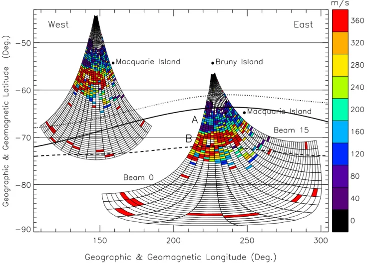
Figure 1 shows the FOV of the TIGER radar mapped in geographic (left) and geomagnetic (right) coordinates. The bore sight of TIGER (beams 7/8) points geographic south, whereas beam 4 (bold) is closely aligned with the magnetic meridian (226◦E). In the fast (normal) common mode of op-eration, TIGER performs one sequential 16-beam scan from east (beam 15) to west (beam 0), integrating for 3 s (7 s) on each beam. Hence, a full scan takes 48 s (112 s), with succes-sive scans synchronised to the start of 1-min (2-min)
bound-M. L. Parkinson et al.: Decametre-scale irregularities in the sub-auroral, auroral, and polar cap ionosphere 1849
Fig. 1. The field-of-view (FOV) of the TIGER radar mapped to geographic (left) and geomagnetic coordinates (right), both drawn on the
same grid to emphasise differences. The magnetic meridian pointing beam 4 and the eastern beam 15 are shown in bold. Shaded pixels represent ionospheric echoes with spectral widths < 200 m s−1(light) and > 200 m s−1(dark) recorded during the full scan commencing 17:16 UT on 5 September 2000. The location of auroral oval boundaries given by the Starkov (1994b) model for AL = −172 nT (Kp=3)
are superimposed: poleward boundary of the discrete aurora (dashed curve), equatorward boundary of the discrete aurora (solid curve), and equatorward boundary of the diffuse aurora (dotted curve).
aries. Individual beams in the scan are separated by 3.24◦, and the full scan spans 52◦of azimuth.
Figure 1 illustrates the large difference between the geo-graphic and magnetic FOVs; some of the underlying dynam-ics will be characteristic of a high mid-latitude station (e.g. radio propagation, insolation, and D-region absorption), yet others will be characteristic of the sub-auroral, auroral, and polar cap ionosphere. Figure 1 also illustrates the presence of two separate populations of ionospheric echoes, “A” and “B”, with low and high spectral widths, respectively, (to be defined). Model auroral oval boundaries given by Starkov (1994b) have been superimposed with beam 4 located at mid-night MLT. The auroral electrojet index AL = −172 corre-sponding to Kp =3 used to drive the model was calculated using the conversion given by Starkov (1994a). The Starkov model has been tested against real data, but other models would give similar results.
If occurrence statistics were compiled for all 16 beams
combined, it would be difficult separating geophysical and geometric dependencies. Hence, we compiled occurrence statistics for beams 4 and 15 (Fig. 1, bold), thereby revealing the most interesting aspects of data recorded on all beams. For example, beam 4 was chosen because it points down the magnetic meridian, providing an overview of dynamics oc-curring in the sub-auroral, auroral, and polar cap ionosphere (−57◦3to −88◦3). Assuming the E × B/B2drift of
F-region irregularities, the corresponding LOS Doppler veloci-ties were also a direct measure of zonal electric fields occur-ring along the meridian.
In contrast, beam 15 (bold) was chosen because its range window extends from latitude −57◦3to −72◦3, providing a detailed view of the nightside sub-auroral and auroral iono-sphere. Beam 15 becomes a zonal, eastward-looking beam at furthest ranges, reaching a maximum latitude of −71.8◦3 (range cell 68) before folding back toward the equator be-yond this range. Thus, beams 4 and 15 are the two most
Table 1. TIGER normal scan data analysed in this study
Summer 1999 and 2000 Autumn 2000 Winter 2000 Spring 2000
02-09, 19-31 December 14-18, 27-29 February 07-18, 24-31 May 14-18, 23-24, 25-28 August 01-03, 13-13, 18-31 January 01-04, 29-31 March 01-04, 05-15, 21-26 June 01-21 September
01-02 February 05-06, 11-12, 14-23 April 01-04, 05-06, 12-20 July 03-17, 20-26 October 09-14, 20-30 November 01-02 May 05-07 November
independent, nearly orthogonal beams in the FOV. Finally, beam 15 is located adjacent to Macquarie Island (−65◦3), a key sub-Antarctic station supporting many ground-based instruments.
In this study we compiled statistics using all available, common mode data recorded during the sunspot maximum interval, December, 1999 to November, 2000. The actual dates of the measurements are shown in Table 1, subdivided into four seasons redefined to encompass ∼90-day intervals centred on the equinoxes and solstices. This sorting em-phasises the component of seasonal variability controlled by the solar-zenith angle, though other controls may dominate (Basu, 1975).
The radar control programs used to make the normal and fast mode soundings were “normal scan nodata” and “nor-mal scan3”, respectively. We excluded most of the data recorded with other experimental programs to prevent intro-duction of statistical biases.
The default transmission frequency bands for nor-mal scan3 were 14.35 to 14.99 MHz during the “day” (21:00 to 09:00 UT), and 11.65 to 12.05 MHz during the “night” (09:00 to 21:00 UT). A clear frequency search was always performed within these individual frequency bands. How-ever, normal scan nodata invoked a frequency search algo-rithm whenever fewer than 20 beam-range bins contained ionospheric echoes. The program then spent two minutes in-tegrating on beam numbers 2, 6, 10, and 14 at one frequency in each of five different licensed bands spread between 10.1 and 15.6 MHz. The frequency band with the largest num-ber of ionospheric echoes was then adopted in subsequent scans until echoes were detected in fewer than 20 beam-range bins again. The program used the same default bands as nor-mal scan3 whenever fewer than 5 echoes were detected dur-ing a frequency search.
Figure 2 is a histogram showing the roughly trimodal distribution of radar frequencies used throughout the entire study interval. The scale size of ionospheric irregularities corresponding to each of the three dominant peaks were 14.4, 12.3, and 10.3 m, respectively. If it were not for the effects of prohibited frequency bands (shaded), combined with the effects of narrow band interference, the histogram might ap-proximate a bell-shaped or log-normal curve centred some-where between 10 to 12 MHz. The latter is the known fre-quency of maximum radar gain.
Figure 3 shows the diurnal variation of the transmit-ter frequency averaged over 30-min intransmit-tervals, with scat-ter bars superimposed. The daytime frequency tends to be >1 MHz larger, simply to compensate for greater refrac-tion associated with higher daytime electron densities, and thereby increasing the probability of recording useful echoes at greater ranges. Note the resultant discontinuities near 08 and 19 MLT. Figures 2 and 3 are shown because they repre-sent potential biases in our results.
In the common mode of operation, SuperDARN radars calculate the autocorrelation functions (ACFs) of echoes (Hanuise et al., 1993) digitised at 75 range gates starting at 180 km and separated by 45 km (i.e. 180 to 3555 km). The 45-km interval corresponds to the 300-µs width of transmit-ter pulses. The “FITACF” algorithm (Baker et al., 1995) processes the ACFs to estimate the echo power in logarith-mic units of signal-to-noise ratio (i.e. dB), LOS Doppler velocity (m s−1), and the Doppler spectral width (m s−1), for all ranges on every beam. Our version of FITACF re-jected echoes with SNR < 3 dB, flagging the remainder as sea echoes if the Doppler speeds and spectral widths were less than 50 m s−1 and 20 m s−1, respectively, and deter-mined with small errors. In this study, ionospheric echoes were those defined as such by the FITACF algorithm. This identification is reliable in the majority of cases, but some ionospheric echoes are mistaken for ground echoes, and vice versa.
Results shown in the next section are presented in the form of contour plots of echo occurrence and average FI-TACF parameter versus time and range. Beam 4 results are shown in a standard clock dial format using altitude ad-justed corrected geomagnetic coordinates (AACGM) (Baker and Wing, 1989). The range gates were mapped to AACGM latitude using the standard analysis procedure. This assumes a virtual reflection height of 300 km, but with tapering to E-region heights at ranges < 600 km. The difference between MLT and UT for beam 4 was about 10 hours and 46 min, but this difference changes rapidly approaching the geomagnetic pole, where the beam direction veers away from the magnetic meridian.
A total of 1 666 429 (1 357 310) ionospheric echoes were identified on 149 377 (151 310) separate beam 4 (beam 15) soundings, so the major features shown here are statistically significant. Occurrence rates were calculated by counting
M. L. Parkinson et al.: Decametre-scale irregularities in the sub-auroral, auroral, and polar cap ionosphere 1851
Fig. 2. Histogram showing the probability of the radar selecting a particular transmitter frequency during the study interval, December 1999
to November 2000. The radar electronics can operate anywhere between 8 and 20 MHz, but shaded regions correspond to frequency bands we never used because of our RF license restrictions.
the total number of echoes during 15-min intervals of time at each of the 75 ranges, then dividing by the total number of soundings made for a particular category of season, Kp, or the IMF. Thus, 96 times × 75 ranges = 7200 occurrence rates were calculated for each map showing an average di-urnal variation. The total number of echoes in each category was always divided by the actual number of soundings made. Hence, the occurrence rates are “self-normalising” with re-spect to the chosen category.
The Kp index is determined using a network of mid-latitude magnetometers, and is a measure of planetary ge-omagnetic activity. Ideally, measurements made using TIGER, a nightside auroral oval radar, should be sorted ac-cording to the AL index (Davis and Sugiura, 1966), or a lo-cal K index derived from the magnetometer located at Mac-quarie Island. Unfortunately, reliable K or AL indices were not available for this study.
Finally, the IMF data used in this study were 4-min aver-ages measured on board the Atmospheric Composition Ex-plorer (ACE) spacecraft which orbits the L1 libration point located ∼235 Earth radii upstream of the Earth in the so-lar wind. The orthogonal IMF components By and Bzwere
expressed in the geocentric solar magnetospheric (GSM) coordinate system. The IMF components were advected from ACE to the Earth using the geocentric solar ecliptic x-location of the spacecraft and an average solar-wind speed of 370 km s−1. Although this method of advecting the solar-wind conditions is approximate, the same basic statistical re-sults would be obtained when using more refined procedures.
3 Results
3.1 Beam 4 occurrence rates 3.1.1 Seasonal dependence
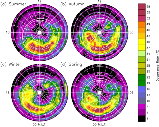
Figure 4 shows the occurrence of beam 4 ionospheric echoes sorted according to season for all Kpvalues. The colour key represents the colour for an occurrence rate of, say, 49% (red), which corresponds to occurrence rates in the range 47.5 to 50.5%. Model auroral oval boundaries (Starkov, 1994b) have been superimposed in each panel using AL = −108 nT (summer) (a), −107 nT (autumn) (b), −131 nT (winter) (c), and −120 nT (spring) (d). These values
corre-Fig. 3. The diurnal variation of transmitter frequency averaged over 30-min intervals of MLT during the study period, December 1999
to November 2000. The scatter bars correspond to ± one standard deviation. The discontinuities in transmitter frequency at 07:46 and 19:46 MLT (21:00 and 09:00 UT) correspond to the transitions between default day and night frequency bands, respectively.
spond to the average Kp values occurring when ionospheric soundings were made, namely 2.28 ± 0.01, 2.27 ± 0.01, 2.56 ±0.01, and 2.43 ± 0.01 in each season, respectively (stan-dard errors are given). Note the poleward edge of the dis-crete auroral oval (dashed curve) delineates a fixed polar cap boundary, but the radar statistics encompass a broad range of geomagnetic activity. Hence, we expect the observed echo distributions to be smeared in latitude with respect to the model boundaries.
Similar patterns of echo occurrence were recorded dur-ing all seasons, but there were some intrigudur-ing differences. For example, the dominant band of echoes observed between ∼−65◦3and −76◦3during the night was confined between ∼20 and 07 MLT during the summer (Fig. 4a), but extended between ∼16 and 08 MLT during the winter (Fig. 4c). The azimuthal extent of this enhanced echo occurrence was in-termediate during the autumn (Fig. 4b) and spring (Fig. 4d). The regions of peak echo occurrence (> 58%; brown) were concentrated after midnight during summer and autumn, be-fore midnight during winter, and nearly symmetric about midnight during spring. However, overall, more echoes were observed post-midnight than pre-midnight.
A lesser patch of mostly polar cap echoes was observed between ∼−70◦3 and −82◦3 on the dusk side, confined between ∼16 and 21 MLT during the winter. The azimuthal extent of this feature contracted toward midnight during autumn and especially spring, and may have completely
merged into the dominant band of nightside auroral echoes during summer. This feature was more distinct in beam 15 observations which showed its azimuthal extent contracted to ∼20 and 23 MLT during summer. Corresponding peak oc-currence rates were found most equatorward during the sum-mer, but were largest and most poleward during the autumn. Relatively few ionospheric echoes were detected in the “dayside ionosphere” (06 to 18 MLT), with occurrence rates mostly < 20%. The minimum occurrence rates were cen-tred on ∼13 MLT during summer and winter, though closer to noon during autumn and spring. Maximum dayside oc-currence rates were observed during winter, and to a lesser extent during autumn, as a consequence of the before-mentioned polar cap echoes extending into the late afternoon. However, the peak occurrence rate was ∼46% for an iso-lated patch of echoes ∼1 h wide, centred near 08:40 MLT and −78◦3during the winter. A similar feature was located near −80◦3during autumn, but the peak occurrence rate dropped to ∼34%. The occurrence rates were lowest of all for this feature during summer. When considering all seasons com-bined, very few ionospheric echoes were detected in the polar cap ionosphere poleward of −80◦3, but especially during 01 to 16 MLT.
Bands of occurrence rates generally < 16% were found between midnight and noon equatorward of −61.8◦3(i.e. range ≤ 630 km), whereas the occurrence rates were gen-erally < 7% between noon and midnight at similar ranges.
M. L. Parkinson et al.: Decametre-scale irregularities in the sub-auroral, auroral, and polar cap ionosphere 1853
Fig. 4. The occurrence rate of beam 4 ionospheric echoes for all Kpvalues detected during (a) summer (days 313 to 035), (b) autumn (days 036 to 126), (c) winter (days 127 to 221), and (d) spring (days 222 to 312). The results are shown versus MLT and magnetic latitude, with noon (12 MLT) at top, and dusk (06 MLT) at right, and the equatorward boundary at −57◦3. Magnetic latitudes −60◦, −70◦, and −80◦3 have been superimposed. No data were acquired poleward of −88◦3. Model auroral oval boundaries have been superimposed (see text).
Table 2. Seasonal changes in beam 4 occurrence rates, range > 630 km
Summer Autumn Winter Spring Total no. echoes 384 257 303 488 457 373 419 371 Total no. beam soundings 40 702 24 164 44 311 40 200 Average occurrence rate (%) 13.70 18.68 15.60 15.01
Standard error (%) 0.19 0.21 0.18 0.18 Peak occur. Rate (%) 71 77 65 65
The peak occurrence rate was ∼20% near 04:30 MLT during the summer, and ∼40% near 06:40 MLT during the winter. When the near-range occurrence rates were averaged for all seasons combined, they were roughly centred near 06 MLT.
The echoes responsible for the occurrence rates at close ranges exhibit the characteristics of meteor echoes (Hall et al., 1997), but echoes from E-region plasma instabilities as-sociated with aurora and sporadic E must also contribute. The corresponding irregularities do not necessarily drift at the ion convection velocity (Hanuise et al., 1991). Hence, in the following analysis we separate echoes into two groups, namely those echoes at ranges ≤ 630 km and those echoes at ranges > 630 km. The latter are thought to correspond to
upper E- and F-region irregularities drifting at the ion con-vection velocity (Villain et al., 1985).
Table 2 shows the total number of echoes observed in each season, the total number of beam 4 soundings in each sea-son, the average occurrence rates, their standard errors, and the peak occurrence rates, all for ranges > 630 km. Variabil-ity in the total number of soundings reflects upon equipment failures (computer crashes, power failures, etc.). There are 64 range bins at ranges > 630 km. Hence, the average oc-currence rate (%) is the average of the 96 times × 64 ranges = 6144 occurrence rates calculated for each season. This av-erage does not equal the total number of echoes divided by the total number of beam soundings, because there was a
dif-Table 3. Seasonal changes in beam 4 occurrence rates, range ≤ 630 km
Summer Autumn Winter Spring Total no. echoes 31 794 14 293 33 673 22 180 Total no. beam soundings 40 702 24 164 44 311 40 200 Average occurrence rate (%) 6.57 4.92 6.60 4.44
Standard error (%) 0.16 0.14 0.20 0.10 Peak occur. Rate (%) 23 25 38 14
Fig. 5. The occurrence rate of beam 4 ionospheric echoes detected during all seasons, and sorted according to geomagnetic activity. (a) Kp =0 to 1, (b) Kp >1 to 2, (c) Kp> 2 to 3, (d) Kp >3 to 4, (e) Kp >4 to 5, and (f) Kp >5 to 6. Model auroral oval boundaries
for (a) AL = −21 nT (Kp ≈1−), (b) AL = −64 nT (Kp ≈2−), (c) AL = −141 nT (Kp ≈3−), (d) AL = −240 nT (Kp ≈4−), (e) AL = −350 nT (Kp≈5−), and (f) AL = −458 nT (Kp≈6−) have been superimposed.
M. L. Parkinson et al.: Decametre-scale irregularities in the sub-auroral, auroral, and polar cap ionosphere 1855
Table 4. Geomagnetic changes in beam 4 occurrence rates, range > 630 km
Kp 0-1 >1-2 >2-3 >3-4 >4-5 >5-6
Total no. echoes 272 966 417 971 440 474 257 342 117 522 30 387 Total no. beam soundings 30 901 40 447 39 682 22 412 10 018 3 462 Average occurrence rate (%) 11.71 15.43 17.01 17.22 17.56 12.34 Standard error (%) 0.16 0.20 0.22 0.23 0.23 0.20 Peak occur. Rate (%) 56 74 80 85 74 82
ferent number of soundings in each of the 15-min intervals and 64 ranges. The standard errors (%) were calculated by dividing the standard deviations of the occurrence rates by √
6144. The peak occurrence rate is simply the maximum occurrence rate of the 6144 occurrence rates.
Table 2 shows that the largest number of echoes was recorded during winter, then spring, summer, and least of all during autumn. However, because of the different num-ber of beam soundings made per season, the average occur-rence rate was largest for autumn, next largest for winter, then spring, and least of all for summer (cf. Fig. 4). On the other hand, peak occurrence rates were largest in autumn, then summer, and then the same during spring and winter. Variations in the averages are more meaningful than varia-tions in the peak values. The standard errors for the averages show that the seasonal changes were statistically significant, but systematic biases not related to the occurrence of iono-spheric irregularities may be present.
Table 3 compiles the same information as Table 2, except it shows the statistics for echoes at ranges ≤ 630 km. There are 11 range bins at ranges ≤ 630 km, so an average occur-rence rate is the average of 96 times × 11 ranges = 1056 occurrence rates. The occurrence rates were largest (∼6.6%) and equal within error limits during summer and winter, and ∼2% lower and comparable during autumn and spring. The peak occurrence rates were largest during winter and least during spring, and similar during summer and autumn. The peak occurrence of 38% occurred at ∼07 MLT during winter (cf. Fig. 4c). In passing, we note this seasonal variation is very similar to the seasonal variation of meteor echoes ob-served at Halley Base, Antarctica (Jenkins et al., 1998).
Lastly, the transmitter pulse set was designed to minimise the detrimental effects of range aliasing. However, the nar-row, circular striations in all panels of Fig. 4 (e.g. the promi-nent ring at ∼−67◦3) correspond to bad ranges in the ACFs calculated using the chosen pulse sequence.
3.1.2 Geomagnetic activity dependence
Figure 5 shows the occurrence rates of ionospheric echoes for all seasons combined and sorted according to the geo-magnetic activity index Kp. As in Fig. 4, peak occurrence rates were usually observed in the nightside auroral and
po-lar cap ionosphere between −65◦3and −76◦3. However, for quiet conditions, Kp = 0 to 1 (a), the patch of mostly polar cap echoes found between 18 and 01 MLT and −73◦3 and −82◦3contained a comparable number of echoes to the band found further equatorward between 22 and 05 MLT, and −70◦3and −76◦3. For K
p >1 to 2 (b) the polar cap fea-ture still contained many echoes, but fewer than the main band of auroral and polar cap echoes. The latter expanded to between 20:30 to 05:00 MLT and −66◦3and −76◦3. For Kp > 2 to 3 (c) and more disturbed conditions (d, e, f) the polar cap feature became indistinguishable as the main band of auroral echoes expanded in longitude and latitude, even extending into the dayside ionosphere.
Overall, peak occurrence rates tended to shift equatorward with Kp, as did the equatorward boundary of the model au-roral oval. However, the peak occurrence rates were partly “trapped” in the latitude range −63◦3to −76◦3, until very disturbed conditions, Kp >4 to 5 (e), when a horseshoe of echoes almost completely encircled the polar cap. For the most disturbed conditions of all, Kp >5 to 6 (f), there was a lot of E- and F-region scatter at close ranges, and scatter from both close and far ranges became very patchy, but lo-cally intense.
Table 4 is in the same format as Table 2, except it shows the changes in average and peak occurrence rates with the Kpindex. The average occurrence rate was smallest during the quietest conditions (Fig. 5a), it grew to a maximum for Kp >4 to 5 (cf. Fig. 5e), and thereafter (Fig. 5f) fluctuated with increasing Kp. For example, the average occurrence rate was 20.2% for Kp > 6 to 7, then 12.8% for Kp > 7 to 8, etc. During the most disturbed intervals (Fig. 5f), the auroral oval began to expand equatorward of the 0.5-hop range window. Auroral E echoes must have begun to mask meteor echoes at close ranges, as well as F-region scatter at greater ranges.
Although not apparent in Table 4, the peak occurrence rates trended from 56% for the quietest intervals to 100% during more disturbed intervals (not listed). This is because the occurrence rates were calculated using a smaller and smaller number of intervals encompassing larger and larger geomagnetic storms. Hence, one sees the patchy distribu-tion of echoes in Fig. 5f. Statistics for echoes at close ranges ≤630 km are not shown because there was no significant
de-Fig. 6. Average power of ionospheric echoes with SNR > 3 dB recorded on beam 4 for all seasons and levels of geomagnetic activity
combined. Equipotential contours calculated using the DICM model (see text) have been superimposed. The minimum electric potential in the dusk cell is −23.4 kV, the maximum potential in the dawn cell is 11.3 kV, and contours are separated by 2.5 kV.
pendency on geomagnetic activity until Kp >5. 3.2 Beam 4 average FITACF parameters 3.2.1 Average powers
Figure 6 shows a map of the average power returned by the FITACF algorithm for ionospheric echoes with SNR > 3 dB, and for all seasons and levels of geomagnetic activity com-bined. When the powers were sorted according to season and Kp, similar variations to those for the occurrence rates were found (e.g. an equatorward expansion with Kp). Aver-age FITACF parameters are not shown in this and subsequent plots if fewer than 2 valid FITACF results were obtained per range-time bin. Thus, many of the small-scale fluctuations are a measure of statistical uncertainty.
Average IMF components for the entire data base were (Bx, By, Bz) = (0.0, 0.6, −0.1 nT). These values were used to drive the DMSP satellite-based Ionospheric Convection Model (DICM) (Papitashvili and Rich, 2002) which outputs high-latitude electric potentials. The results have been super-imposed as equipotential contours representing streamlines of ionospheric flow velocity. In Fig. 6, the flow direction is clockwise in the dusk cell and anticlockwise in the dawn cell, resulting in nearly antisunward flow across the central polar cap.
Figure 6 shows that the main band of echo power >18 dB occurred between 19 and 08 MLT and −62◦3and
−72◦3. Larger echo power > 20 dB occurred between 23 and 07 MLT and equatorward of −70◦3. The maximum in the distribution was centred near 02:45 MLT. The exception was winter when the maximum power was centred on mid-night. The echo power increased rapidly at the equatorward edge of the main band (∼ − 62◦3), maximised at ∼ − 64◦3, and thereafter gradually decreased toward the geomagnetic pole. Minimum average power of 9 dB occurred in the day-side ionosphere between 11 and 16 MLT, diametrically op-posite of the region of maximum power. Overall, the dis-tribution of power was rotated further dawnward and ∼3◦3 equatorward of the main echo occurrence shown in Fig. 4. 3.2.2 LOS Doppler velocities
Figure 7 shows the average LOS Doppler velocities sorted into four categories of the IMF vector in the By–Bz plane, namely By negative, Bz positive (a), By positive, Bz posi-tive (b), By negative, Bz negative (c), and By positive, Bz negative (d). By “positive” and “negative” we mean the IMF components were > 0.5 nT and <−0.5 nT, respectively. The corresponding average IMF components (Bx, By, Bz) were (1.9, −4.0, 3.5 nT) (a), (−1.8, 4.6, 3.6 nT) (b), (1.9, −4.0, −3.6 nT) (c), and (−1.7, 4.5, −3.6 nT) (d), respec-tively. These values were used to drive the DICM and to obtain the equipotentials superimposed in all parts. The flow direction is clockwise in the weak afternoon cell in part (a), and anticlockwise in the weak morning cell in part (b).
Sun-M. L. Parkinson et al.: Decametre-scale irregularities in the sub-auroral, auroral, and polar cap ionosphere 1857
Fig. 7. Average LOS Doppler velocities recorded on beam 4 and sorted into four categories of the IMF in the By−Bz plane: (a) By
negative, Bzpositive, (b) Bypositive, Bzpositive, (c), Bynegative, Bznegative, and (d) Bypositive, Bznegative. Equipotential contours
calculated using the DICM model have also been superimposed. Minimum and maximum potentials occurring in the patterns are as follows: (a) −24.2 kV in the weak afternoon cell, (b) 9.5 kV in the weak morning cell, (c) −52.8 kV in the dusk cell and 26.8 kV in the dawn cell, and (d) −38.0 kV in the dusk cell and 31.2 kV in the dawn cell. Contours are separated by 5 kV.
ward flows are known to occur more often in the dayside ionosphere under Bznorthward conditions.
Figure 7 basically shows that the familiar cross polar jet was most developed for Bz negative conditions (c), (d). Note the dayside region of large poleward velocities (brown; ∼<−240 m s−1) was most extensive for B
y positive con-ditions (d). These velocities correspond to flows entering the convection throat during 08 to 14 MLT at ∼ − 78◦3. The nightside region of large equatorward velocities (purple; ∼240 m s−1) was most extensive for By negative conditions (c). These velocities correspond to flows exiting the polar cap during 21 to 24 MLT. They produced the extensive regions of moderate, equatorward LOS velocity (blue; ∼120 m s−1) during 19 to 02 MLT poleward of ∼ − 68◦3.
When sorted according to season, the maps of average LOS Doppler velocity show variations similar to those in Fig. 7. However, the region of large poleward velocities centred in the pre-noon sector were clearly more extensive
during summer, then spring, winter, and least of all during autumn.
3.2.3 Doppler spectral widths
Figure 8 shows the average Doppler spectral widths for all seasons and levels of geomagnetic activity combined. The tendency for small and large spectral widths to sometimes alternate in bands separated by ∼3◦3wide is probably an artifact associated with the pulse set used to measure the ACFs, and the numbers subsequently returned by the FI-TACF algorithm. Ideally, these artifacts should be quantified by modelling the pulse set behaviour, and then deconvolved from the observations. However, all the major features to be described were geophysical and reproducible using subsets of the entire data base.
The largest spectral widths, > 350 m s−1 (brown), were concentrated in the pre-noon polar cap ionosphere at
Fig. 8. Average Doppler spectral widths
recorded on beam 4 for all seasons and Kp values combined. Magnetic
L-shells of 4, 5, 6, 7, and 8 have been su-perimposed, as well as the same equipo-tential contours superimposed in Fig. 6.
∼−80◦3. However, an arc of large spectral widths >300 m s−1(orange) extended into the nightside ionosphere between 23 and 06 MLT. The spectral widths declined quickly equatorward of −73◦3 near noon (and −70◦3 near dawn), whereupon they were < 160 m s−1(blue) across much of the remaining dayside ionosphere. Similarly, the nightside spectral widths declined quickly near midnight, de-creasing from ∼260 m s−1at −70◦3to ∼100 m s−1 equator-ward of −67◦3. There was a significant “bite out” in spectral widths to values < 220 m s−1centred on dusk, but extending from 15 to 21 MLT poleward of 67◦3.
There was an ∼2 to 3◦3wide “trough” in spectral width (< 160 m s−1) centred on ∼−66◦3and nearly encircling the entire 24 h of MLT. The spectral widths again increased to values > 160 m s−1 equatorward of −63◦3, especially be-tween 16:00 and 01:30 MLT. A thin band of large spectral widths > 200 m s−1was centred pre-dawn, between 02:30 to
07:30 MLT and −60◦3and −63◦3.
When the results shown in Fig. 8 were sorted according to season (not shown), similar relative variations were appar-ent. However, there was a significant change in the extent of the pre-noon region with large spectral widths, from most extensive during spring, then summer, winter, and least of all during autumn. During spring the region of average spectral width > 240 m s−1extended in longitude to encompass the high-latitude ionosphere poleward of −70◦3, except within ∼17 to 21 MLT.
When the results shown in Fig. 8 were sorted according to Kp(not shown), the spectral widths behaved similar to the occurrence of echoes (Fig. 5). The relative variations in spec-tral width were most like the Fig. 8 variations for moderately disturbed conditions, Kp =2+ to 3. For Kp =0 to 1, the region of large spectral widths > 300 m s−1was concentrated
in the sector 23 to 07 MLT at ∼ − 74◦3. As Kp increased the regions of large spectral width expanded into the pre-noon polar cap ionosphere, and equatorward. For the most disturbed conditions, there was a strong tendency for the re-gions of large spectral width to expand further until there was an almost symmetric distribution about the AACGM pole. However, there was still evidence for the dusk bite out.
When the results shown in Fig. 8 were sorted according to the IMF (not shown), the high-latitude regions of large spec-tral widths were least extensive for Bypositive, Bzpositive, and most extensive for By negative, Bz negative. The dusk bite out in spectral width was also more prevalent for Bz pos-itive.
Finally, Fig. 8 is annotated with the approximate locations of some important magnetospheric boundaries and regions. These annotations will be discussed in Sect. 4.3.
3.3 Beam 15 occurrence rates
Figure 1 shows how beam 15 provided a detailed view of the nightside sub-auroral and auroral ionosphere, becoming an eastward-looking beam very sensitive to zonal flows at the furthest ranges. Occurrence statistics for beam 15 ob-servations were presented by Parkinson et al. (2002a). Here we further analyse beam 15 observations in the context of beam 4 observations, to investigate the behaviour of iono-spheric scatter with very low spectral width.
First consider Fig. 9 which shows histograms of echo oc-currence versus Doppler spectral width recorded on beam 15 (solid curve) and beam 4 (dotted curve) for all seasons and levels of geomagnetic activity combined. More echoes were observed on beam 4 than beam 15 (660 646 versus 624 051). For each beam there were two distinct populations of iono-spheric echoes, “A” and “B”. Population A included echoes
M. L. Parkinson et al.: Decametre-scale irregularities in the sub-auroral, auroral, and polar cap ionosphere 1859
Fig. 9. Histograms of the number of ionospheric echoes versus
Doppler spectral width recorded on beam 15 (solid curve) and beam 4 (dotted curve) during all seasons and Kpvalues combined.
A bin size of 2 m s−1was used.
with low spectral width < 38 m s−1and had a mode value of ∼9 m s−1(bin size of 2 m s−1). They constituted 16.7% and 9.8% of the echoes observed using beam 15 and beam 4, re-spectively. Population B included echoes with moderate to very large spectral width ≥ 38 m s−1, and had a mode value of only ∼70 m s−1.
Although the distribution functions for populations A and B must overlap, population A was completely dominant be-neath the critical value 38 m s−1. More echoes with spec-tral width < 38 m s−1were recorded on beam 15, and more echoes with spectral width > 38 m s−1 were recorded on beam 4. Population A, in particular, may have been con-taminated by sea echoes.
Figure 10 compiles the occurrence of population A echoes observed on beam 15 versus UT and group range, with cor-responding magnetic latitudes superimposed. The observa-tions were compiled in this way to emphasise variaobserva-tions due to changing propagation conditions. These would be less ap-parent if the results were compiled in the polar plot form of beam 4, because beam 15 traverses 68◦of longitude (∼4.5 h of MLT), and only achieves a maximum poleward latitude of −71.8◦3.
Nominal values of MLT in the ionosphere above Mac-quarie Island, located just to the east of beam 15, are shown at the top of Fig. 10. Similar to Fig. 4, model auroral oval boundaries are also superimposed in each panel using AL = −109 nT (a), −108 nT (b), −131 nT (c), and −120 nT (d). These values correspond to the average Kp values oc-curring when beam 15 soundings were made, namely 2.30 ± 0.01 (a), 2.28 ± 0.01 (b), 2.56 ± 0.01 (c), and 2.43 ± 0.01 (d).
Figure 10 shows that the occurrence of population A echoes observed on beam 15 was similar to the occurrence of echoes with any spectral width on beam 4 (Fig. 4). How-ever, the peak occurrence rates were displaced further toward
Table 5. Seasonal changes in population A echoes, beam 15, range > 630 km
Summer Autumn Winter Spring Total no. echoes 76 880 68 038 96 532 67 443 Total no. beam soundings 40 231 26 214 44 384 40 481 Average occurrence rate (%) 2.44 3.58 2.93 2.07
Standard error (%) 0.05 0.06 0.05 0.04 Peak occur. Rate (%) 27 36 21 23
dawn and the equator than in Fig. 4. Specifically, the main band of echoes observed on beam 15 (> 8%; karki) was con-centrated between 23 and 07 MLT and −63◦3and −67◦3. Hence, these echoes were mainly concentrated in the post-Harang diffuse auroral oval, but also in the discrete auroral oval and sub-auroral ionosphere. Very few of these echoes were from the polar cap ionosphere.
Like the occurrence of echoes recorded on beam 4 (Fig. 4), the azimuthal extent of the dominant band of echoes ob-served on beam 15 was least during summer, greatest dur-ing winter, and intermediate durdur-ing autumn and sprdur-ing. A lesser patch of mostly auroral oval echoes was observed be-tween −65◦3 and −72◦3 on the dusk side, confined be-tween ∼15 and 21 MLT during the winter. The azimuthal extent of this feature contracted toward midnight during au-tumn and spring, and most of all during summer.
The bands of echoes observed with occurrence rates mostly < 6% equatorward of −60◦3correspond to backscat-ter from meteor trails, as well as E- and F-region plasma in-stabilities associated with aurora and sporadic-E.
Table 5 shows the total number of population A echoes (spectral width < 38 m s−1) observed at ranges > 630 km in each season, the total number of beam 15 soundings in each season, the average occurrence rates, their standard errors, and the peak occurrence rates. Because we are only consider-ing echoes with a spectral width < 38 m s−1, the occurrence
rates are much lower than those given for beam 4 (Table 2). The average occurrence rates were largest for beam 15 during autumn, then winter, summer, and least of all for spring. On the other hand, peak occurrence rates were largest in autumn, then summer, spring, and winter.
3.4 Beam 15 average LOS Doppler velocity
Figure 11 shows the average LOS Doppler velocities for beam 15 ionospheric echoes with any spectral width and Kp value. The results have been sorted according to season, and the same model auroral oval boundaries used in Fig. 10 have been superimposed. The dominant feature in all seasons is the transition from large approaching (blue) to large receding (brown) Doppler velocities centred near 22 MLT at −70◦3, but occurring later at closer ranges (lower latitude). This
fea-Fig. 10. The occurrence rate of population A echoes recorded on beam 15 during (a) summer, (b) autumn, (c) winter, and (d) spring for all Kp
values. The results are shown versus UT and group range, with magnetic latitudes −60◦, −65◦, and −70◦3superimposed. Nominal values of MLT in the ionosphere above Macquarie Island are given at top. Similar to Fig. 4, model auroral oval boundaries for (a) AL = −109 nT (Kp =2.30), (b) AL = −108 nT (Kp = 2.28), (c) AL = −131 nT (Kp = 2.56), and (d) AL = −120 nT (Kp = 2.43) have also been
superimposed.
ture corresponds to the transition from westward to eastward return flows at the low-latitude limit of two-cell convection patterns, and is closely related to the Harang discontinuity, a feature normally identified using magnetometer data.
The colour coding used in Fig. 11 suggests large aver-age westward flows were more extensive than large east-ward flows. Indeed, some very large westward flows (> 300 m s−1) overlapped the diffuse auroral oval, and ex-tended equatorward into the sub-auroral ionosphere before magnetic midnight. For example, during summer there was an “island” of large westward flow centred near 21 MLT and −62.5◦3. Similar sub-auroral flows persisted during autumn and especially spring, but were concentrated at higher lati-tude during winter.
When sorted according to geomagnetic activity, the strong westward flows were absent at sub-auroral latitudes for Kp = 0 to 1. The auroral flows intensified with increasing Kp, becoming prevalent at sub-auroral latitudes for Kp >3 to 4 (and similarly for Bzstrongly negative). When only the echoes with spectral width < 38 m s−1were considered, the
region of large westward flow before midnight shifted equa-torward into the sub-auroral ionosphere.
Note that beam 15 has a strong meridional component at latitudes equatorward of −65◦3. Hence, the large approach-ing velocities may have been due to the cross-polar jet. How-ever, Fig. 7 shows that the cross-polar jet was usually extin-guished in the 20 to 22 MLT sector equatorward of −62.5◦3. Thus, the large approaching velocities observed on beam 15 were indeed zonal and towards the west.
4 Discussion
4.1 Beam 4 diurnal and Kpvariations
From the auroral oval boundaries (Starkov, 1994b) super-imposed in Fig. 4, we infer that most of the ionospheric echoes observed at ranges > 630 km on beam 4 were from decametre-scale irregularities drifting in the nightside dis-crete auroral and polar cap ionosphere. However, many echoes were from irregularities in the nightside diffuse
au-M. L. Parkinson et al.: Decametre-scale irregularities in the sub-auroral, auroral, and polar cap ionosphere 1861
Fig. 11. Average LOS Doppler velocities for beam 15 ionospheric echoes with any spectral width and Kpvalue recorded during (a) summer, (b) autumn, (c) winter, and (d) spring. The same model auroral oval boundaries used in Fig. 10 have been superimposed.
roral and sub-auroral ionosphere. There was also a tendency for large occurrence rates to shift pre-midnight for more dis-turbed conditions, Kp >3 (d), (e), and (f). Figure 5 showed the location of the main band of nightside echoes tended to expand in longitude and equatorward with increasing levels of geomagnetic activity. For the quietest conditions, Kp=0 to 1 (Fig. 5a), most of the echoes were associated with the po-lar cap ionosphere, but for Kp >2 to 3 (Fig. 5c), and higher levels of activity, the majority of the echoes were associated with the expanded discrete auroral oval.
These results can be reconciled with the Kp dependency observed for the Goose Bay radar in the Northern Hemi-sphere (Ruohoniemi and Greenwald, 1997). They found that the highest occurrence rates were observed in the nightside ionosphere for quiet conditions, and in the afternoon for dis-turbed conditions. This is because the Goose Bay radar is located 7.3◦3further poleward, and the main region of ir-regularity production expands equatorward of its FOV during disturbed conditions. They also argued that echoes were sup-pressed in the morning sector during disturbed conditions be-cause of enhanced absorption due to energetic electron pre-cipitation. The same effect occurs in the TIGER data, but it is weaker (Fig. 5d, e, and f), again probably because TIGER is located further equatorward of the auroral oval.
Figures 4, 5, and 10 show there was a tendency for
more echoes to be observed post-midnight in the main band of auroral and polar cap echoes. The average backscatter power (Fig. 6) also maximised post-midnight, between 23 and 07 MLT, and was aligned with the leading edge of the main band of peak occurrence rate (∼−65◦3). Overall, more echoes were recorded with higher SNR post-midnight. What is the major cause of this feature in the observations?
A number of factors will affect the observation of iono-spheric echoes with SuperDARN radars. They include the design and operation of the radar, changes in HF propaga-tion condipropaga-tions, and changes in the amplitude and number density of ionospheric irregularities. Changes in the opera-tion of the radar cannot explain the occurrence of stronger echoes post-midnight because the radar was operated in the same way throughout the night. It is difficult to quantify the relative importance of changing propagation conditions without knowledge of the real ionospheric conditions com-bined with ray tracing. However, the fminvariations in iono-grams recorded at high mid-latitude stations show that ab-sorption due to insolation tends to decrease at sunset, and not near midnight. Moreover, D-region absorption due to elec-tron precipitation increases post-midnight. Thus, it seems reasonable to speculate that stronger echoes were observed post-midnight, largely because of more intense irregularity formation.
Tsunoda (1988) provided a possible explanation for why stronger irregularities should be observed post-midnight. The linear growth rate for the E × B instability (Linson and Workman, 1970) is γ0=V0/Lfor ω νin, where V0is the
“slip” velocity, or the magnitude of the plasma velocity mi-nus the neutral wind velocity. L is the gradient scale length of plasma density, ω = ωr +j γ0is the wave frequency, and
vin is the ion-neutral collision frequency. Tsunoda (1988) explains how gradient drift waves should grow in proportion to the slip velocity, since if V0= 0, no Pedersen currents can
flow to provide the polarisation fields which destabilise the plasma density. Larger growth rates might lead to the forma-tion of more intense irregularities, but this is still a point of conjecture.
Figures 29, 30, and 31 reproduced in Tsunoda (1988) sug-gest that larger slip velocities occur post-midnight, support-ing his prediction that stronger irregularity production should occur post-midnight. Conde and Innis (2001) recently re-ported more thermospheric gravity-wave perturbations occur post-midnight, also implying greater slip velocities. Parkin-son et al. (2002b) presented a case study (see their Fig. 3) which showed sudden increases in backscatter power in as-sociation with velocity transients occurring past the Harang discontinuity. The backscatter power also tended to increase in proximity to the poleward boundary of the auroral oval.
Note that larger slip velocities should tend to occur when-ever ionospheric electric fields or neutral winds change rapidly, since it takes some time for an equilibrium to be achieved between the ion and neutral gas motions. More-over, larger slip velocities should also tend to occur wher-ever the ionospheric electric fields vary rapidly in a spatial sense, such as near the poleward boundary of the auroral oval (see Tsunoda, 1988). Thus, strong ionospheric echoes might be observed by SuperDARN radars, even during periods of steady-state convection. A statistical analysis of echo occur-rence sorted according to spatial and temporal variability in the ionospheric convection may help to address these issues. Because of the short lifetime of decametre irregularities, Fig. 4 of this paper suggests that the most active source re-gion for the irregularities observed using TIGER was the nightside ionosphere overlapping the poleward edge of the auroral oval, and extending into the discrete auroral oval. Figure 5 suggests that this source region tended to shift equa-torward and pre-midnight into the discrete auroral oval dur-ing more disturbed intervals. Although the post-midnight echoes may have been partly suppressed by enhanced ab-sorption (Ruohoniemi and Greenwald, 1997), we speculate that the trend was also caused by more slip-velocity tran-sients developing pre-midnight because of ionospheric sub-storms.
Although the average occurrence rates (Table 2) for the largest Kp values were only representative of a small num-ber of storms, they clearly showed that localised “hot spots” of echo occurrence were often observed, even during major storms when there was intense particle precipitation. Iono-spheric absorption due to particle precipitation reduced the echo occurrence in transient, spatially localised episodes.
However, overall, the echo occurrence remained very high during major storms, perhaps because of strong and frequent slip-velocity transients.
4.2 Beam 4 propagation effects
Figure 4 showed that the enhanced echo occurrence actually consisted of two separate regions, a main one found between ∼−65◦3and −76◦3and persisting beyond magnetic mid-night, and a lesser patch of mostly polar cap echoes observed between ∼−70◦3and −82◦3near dusk. The familiar equa-torward expansion of the auroral oval with MLT (for the same level of geomagnetic activity) can only partly explain these two echo regions. This is because one of them clearly lay well into the polar cap.
Recall that variability in the refraction of the radio waves influences the observation of ionospheric echoes. The iono-spheric electron density encountered along the ray path deter-mines the preferred range windows at which the radio waves achieve normal incidence with magnetically field-aligned ir-regularities (Villain et al., 1985). To produce observable echoes, these preferred range windows must also correspond to ionospheric regions associated with intense irregularity production.
However, the location of the preferred range windows is variable, and to some extent decametre irregularities will be observed wherever they occur. This is because they form as a part of a cascade process: 10-m scale irregularities form on the gradients of 100-m scale irregularities, which form on the gradients of 1-km scale irregularities, etc. Hence, the 10-m scale irregularities will often form in the presence of large-scale gradients required to refract the radio waves to normal incidence.
The lesser patch of mostly polar cap echoes observed at higher latitude on the dusk side corresponds to a preferred range window due to 1.5-hop propagation, and the main band of echoes observed at lower latitude and later MLT corre-sponds to a preferred range window due to 0.5-hop propa-gation. In a statistical sense, these two preferred range win-dows overlap. However, the lesser region of mostly polar cap echoes tended to occur during quiet conditions because the main auroral oval expanded equatorward into the pre-ferred range window due to 0.5-hop propagation during more disturbed conditions. Presumably, echoes were usually not observed at dusk via 0.5-hop propagation during quiet con-ditions because of weak irregularity production in the sub-auroral ionosphere where insolation was more direct.
The preceding interpretation was confirmed by (i) the sim-ilar effects observed at simsim-ilar group ranges on beam 15, (ii) the sudden decrease in operating frequency at 19 MLT (Fig. 3) which subsequently favoured observation of echoes via 0.5-hop propagation, (iii) elevation angle data (not shown) which suggested that the two echo regions were ob-served via different propagation modes, and (iv) examination of the behaviour of 1.5-hop ionospheric echo traces with re-spect to 1.0-hop sea-echo traces in range-time plots for indi-vidual days.
M. L. Parkinson et al.: Decametre-scale irregularities in the sub-auroral, auroral, and polar cap ionosphere 1863 The behaviour of the sea-echo traces was consistent with
the behaviour of the ionospheric parameters hmF2 and foF2 in ionograms recorded nearby TIGER at Hobart (147.3◦E, 42.9◦S geographic). Past sunset, hmF2 increased and foF2 decreased, and 1.0-hop sea-echo traces gradually receded to great ranges until they were lost. Ionospheric echoes in the preferred range window due to 1.5-hop propagation were ob-served until this happened. Then nightside auroral E- and F-layers began to support the observation of echoes via 0.5-hop propagation.
4.3 Beam 4 seasonal variations
Some of the echoes observed using TIGER were associated with the pre-noon greater cusp, consisting of the true cusp, cleft, and mantle (Newell and Meng, 1992). For example, there was a peak occurrence rate of ∼46% near 08:40 MLT and −78◦3during winter (Fig. 4c). This feature was centred poleward of the poleward edge of the auroral oval, so many of the corresponding irregularities may have been concentrated in the mantle rather than the cusp proper. Why were so few dayside echoes observed, especially when the cusp is known to be such an intense source of irregularity production?
The true ranges of the auroral and polar cap ionosphere were greater during the daytime. Except during very dis-turbed conditions, dayside echoes were probably observed via 1.5- and 2.5-hop propagation, resulting in greater diver-gent power losses. D-region absorption due to insolation was also probably greatest during the daytime (cf. Fig. 6), just past noon (∼13 MLT) in summer, when the Sun was high in the sky, and least during the early morning in the win-ter when the Sun was beneath the horizon. However, Ruo-honiemi and Greenwald (1997) argued that suppression of large-scale plasma density gradients during the summer was the main cause of a similar wintertime maximum in dayside cusp echoes observed in the Northern Hemisphere.
The contraction of the lesser region of mostly polar cap echoes from dusk in winter toward later MLT in summer (Fig. 4; Sect. 3.1.1) is consistent with the well-known sea-sonal variation in F-region sunset time. The location of the terminator is a very important consideration because decades of ionosonde measurements have shown that the ionosphere is smoother when directly illuminated. There is a sound theo-retical basis for these observations. First, the large-scale gra-dients in plasma density required for production of smaller scale irregularities are suppressed by insolation. Second, the presence of a conducting E region reduces the lifetime of ir-regularities in the F-region by allowing the cross-field plasma diffusion to proceed at the faster ion rate, rather than the slower electron rate (Vickrey and Kelley, 1982; Kelley et al., 1982). Hence, all else being equal, irregularities “dissolve” faster in the presence of a conducting E-region.
Table 2 showed the average occurrence rate of ionospheric echoes at ranges > 630 km was greatest during autumn (18.7%), then winter (15.6%), spring (15.0%), and least of all during summer (13.7%). The variation of beam 15 echoes was similar and largely determined by variations in the
oc-currence of irregularities in the nightside auroral oval. Al-though relatively small, the variations were statistically sig-nificant and similar to the familiar, but unexplained, sea-sonal variation in auroral activity, with peak activity near the March (austral autumn) equinox. We note that if reliable AL indices were available for our study period, they might have shown peak auroral activity, and thus irregularity production, near the March equinox.
Scintillation of VHF signals traversing the ionosphere and received with ground-based antennas are caused by iono-spheric irregularities of scale size ∼250 m to 1 km. Typical power spectra of ionospheric irregularities show a cascade of irregularities from these scale sizes down to the decametre-scale size observed using HF backscatter radar (Tsunoda, 1988). Hence, we expect there to be a correspondence be-tween the occurrence of ionospheric irregularities implied by the two measurement techniques.
Indeed, the diurnal and seasonal variation of scintilla-tion index observed at Narssarssuaq, Greenland (+63◦3) (Aarons, 1982), (see Fig. 19 therein) resembled the varia-tion of occurrence rate shown in Table 2. The Narssarssuaq scintillation index maximised in the months of March and April, and then slowly declined throughout the remainder of the year, reaching a minimum during November and Decem-ber. A similar but weaker seasonal behaviour was observed using TIGER, even though the stations reside in different lon-gitude sectors, and opposite hemispheres. The diurnal max-ima also had similar character. However, the diurnal scin-tillation maxima were centred pre-midnight (∼23 MLT) at Narssarssuaq, whereas the diurnal maxima of TIGER echoes tended to occur post-midnight.
Basu (1975) investigated the UT seasonal variations of au-roral zone activity by compiling average AL indices. Basu’s analysis revealed variations in auroral activity which were at-tributed to variations in the plane of symmetry of the plasma sheet with respect to the solar magnetospheric equatorial plane. The seasonal variations in AL were consistent with the seasonal variation in Narssarssuaq scintillations. The sea-sonal variations were strongest for auroral stations in the geo-graphic meridian containing, or opposite to, the geomagnetic pole. It is likely AL is also a measure of decametre irreg-ularity production, as well as scintillation activity. Consult-ing Fig. 2 of Basu (1975), there should be a relatively weak seasonal variation in echo occurrence observed at a station where magnetic midnight occurs at ∼14:00 UT. This is con-sistent with the relatively weak seasonal variation of TIGER echoes.
It is well known that changes in the dipole tilt angle regulate the transfer of solar-wind energy into the cou-pled magnetosphere-ionosphere-thermosphere system (Rus-sell and McPherron, 1973). However, the system is very complex and many factors must be considered to explain the peak irregularity production near autumn equinox. These factors include variations in conditions satisfying the anti-parallel merging hypothesis (Crooker, 1979), and variations in the ionospheric conductivity due to changes in the solar-zenith angle and particle precipitation. The conductivity of
the conjugate ionosphere will also affect the closure of field-aligned currents. Aurora, intense electric fields, and thus irregularity production concentrate in regions of low iono-spheric conductivity (Newell et al., 2001).
In this section we outlined two different kinds of seasonal variation in irregularity occurrence. Earlier we discussed the direct role of insolation in producing D-region absorption, and concentrating the regions of strong irregularity produc-tion in the nightside ionosphere. This kind of seasonal vari-ation is asymmetric across hemispheres, that is, the region of strongest irregularity production is greatest in the winter hemisphere. Then we discussed the familiar variation in au-roral activity which maximises in the austral autumn (boreal spring). This contribution is symmetric across hemispheres. Both the asymmetric and symmetric contributions help to ex-plain the seasonal variations revealed in Fig. 4.
4.4 Beam 4 LOS Doppler velocities and spectral widths Figure 7 showed the average LOS Doppler velocities sorted according to the IMF vector, with DICM equipotentials su-perimposed to help show how the radar observations were consistent with a basic two-cell convection pattern with a cross polar cap jet most developed under Bz negative con-ditions. Further detail can be compared; for example, Fig. 7c shows a region of near zero LOS velocity (karki) centred near ∼04 MLT and −75◦3. This implies the location of the centre of the dawn convection cell, in better agreement with the re-sults of the DICM model than the DMSP-calibrated IZMEM model (Papitashvili and Rich, 2002; see their Figs. 2 and 7). However, such comparisons are best made using Super-DARN convection potentials derived using LOS Doppler ve-locities measured by all the SuperDARN radars combined (Shepherd and Ruohoniemi et al., 2000).
When average Doppler parameters were sorted according to season (not shown) they revealed that the region of large poleward velocities and spectral widths centred in the pre-noon ionosphere were more extensive during summer, then spring, winter, and least of all during autumn. This is nearly opposite to the seasonal variation in echo occurrence in the pre-noon ionosphere, namely a maximum during winter, then autumn, spring, and least of all during summer. To first or-der, one might expect the echo occurrence (and average spec-tral widths) to increase with convection velocity. However, a deeper analysis of the conditions affecting the growth and decay of irregularities is required. This includes determining the slip velocities, and allowing for enhanced conductivity due to direct insolation which maximises in summer.
Figure 8 showed the average Doppler velocity spectral widths for all seasons and Kp values combined. Variations in the spectral widths may represent genuine variations in the hydromagnetic wave activity (Andr´e et al., 1999, 2000a, 2000b) or small- to medium-scale turbulence in the plasma convection. The region of large spectral widths extended into the pre-noon ionosphere and intensified with increasing Kp (or Bz southward) conditions (not shown). This suggests dayside reconnection may have driven the hydromagnetic
wave activity or turbulence responsible for the large spectral widths.
Andr´e et al. (2000b) also showed how large-scale gradi-ents and especially strong flow shears in the plasma convec-tion will enhance the spectral widths. However, the average spectral widths shown in Fig. 8 were observed on the merid-ional beam 4 which was never parallel to the normal dawn or dusk convection reversal boundary (CRB). Nevertheless, strong flow shears must have occurred throughout the study interval, and may explain some of the larger spectral widths affecting the statistics.
Well-known ionospheric locations mapping to the greater cusp, polar cap (PC), and CRB were superimposed in Fig. 8. When the spectral widths are plotted versus group range and time for TIGER beam 4, a persistent latitudinal decrease in nightside spectral width is often observed (Parkinson et al., 2002b). The spectral width boundary is usually very sharp, occurring within two range gates or ∼90 km, and its loca-tion expands equatorward or contracts poleward, depending on geomagnetic activity. The nightside spectral widths de-creased gradually in Fig. 8, because they were averaged over the non-stationary behaviour of the spectral width boundary revealed in case studies. Nevertheless, the gradual statistical boundary still expanded equatorward with Kp.
Parkinson et al. (2002b) also argued that (i) the spectral width boundary mapped to the open-closed magnetic field line boundary (OCB) in the evening and midnight sector, (ii) the scatter with low spectral width just equatorward of the spectral width boundary mapped to the auroral oval, and (iii) the equatorward limit of this scatter mapped to the poleward wall of the main ionospheric trough. Hence, we have in-ferred nominal locations of the OCB, plasma sheet boundary layer (PSBL), central plasma sheet (CPS), and plasmapause in Fig. 8. For example, we have placed the plasmapause near L =4.
Note that because the spectral width boundary is so sharp in case study data, it is well defined using any spectral width threshold between ∼50 and 200 m s−1. However, Fig. 9
sug-gests that the use of a lower (higher) threshold will more ex-clusively select population A (B) echoes only.
Large spectral widths were observed encircling the dawn sector but not the dusk sector. This suggests that there may be more hydromagnetic wave activity or turbulence in the dawn sector. The bite out in large spectral widths centred on dusk may be related to the dusk bulge of the plasmapause which disappears during geomagnetic storms, or large Kp, as was observed.
Lastly, we speculate that the thin band of large spectral widths > 200 m s−1found between 02:30 to 07:30 MLT and −60◦3and −63◦3may be associated with strong F-region irregularities forming high in the pre-sunrise trough when electron densities plummet.
4.5 Beam 15 results
Figure 9 revealed two separate populations of ionospheric echoes, “A” and “B”, having low and moderate to very