HAL Id: halshs-00570477
https://halshs.archives-ouvertes.fr/halshs-00570477
Preprint submitted on 28 Feb 2011
HAL is a multi-disciplinary open access archive for the deposit and dissemination of sci-entific research documents, whether they are pub-lished or not. The documents may come from teaching and research institutions in France or
L’archive ouverte pluridisciplinaire HAL, est destinée au dépôt et à la diffusion de documents scientifiques de niveau recherche, publiés ou non, émanant des établissements d’enseignement et de recherche français ou étrangers, des laboratoires
Deforestation and the Real Exchange Rate
Jean-Louis Arcand, Patrick Guillaumont, Sylviane Guillaumont Jeanneney
To cite this version:
Jean-Louis Arcand, Patrick Guillaumont, Sylviane Guillaumont Jeanneney. Deforestation and the Real Exchange Rate. 2011. �halshs-00570477�
November 2005
Deforestation and the Real Exchange Rate
Abstract
Deforestation is a phenomenon that has largely been concentrated in the developing world. We construct a theoretical model of deforestation that focuses on the factors a¤ecting the incen-tives to transform forested land into agricultural land. We show that: (i) lower discount rates and stronger institutions decrease deforestation; (ii) depreciations in the real exchange rate in-crease deforestation in developing countries whereas the opposite obtains in developed countries; (iii) paradoxically, better institutions may exacerbate the deleterious impact of depreciations in developing countries. These hypotheses are tested on an annual sample of 101 countries over the 1961-1988 period, and are not rejected by the data. Our results suggest that short-term macroeconomic policy, institutional factors, and the interaction between the two, are potentially important determinants of environmental outcomes.
Keywords: deforestation, real e¤ective exchange rate, institutions. JEL: O13, Q23, F31, F41
“La forêt ici manque et là s’est agrandie,” Victor Hugo, Les Rayons et les Ombres
“Fear not till Birnam wood do come to Dunsinane,” William Shakespeare, Macbeth
1
Introduction
In recent years, deforestation, particularly in developing countries, has been of increasing concern, mainly because of widespread fears of global warming and declining biodiversity. The 2003 World Development Report states that “one-…fth of all tropical forests have been cleared since 1960. According to the Food and Agriculture Organization of the United Nations (FAO), deforestation has been concentrated in the developing world. At the same time, forest cover in industrial countries is stable or even increasing slightly.”1 2
The aim of this paper is to understand why forest cover is decreasing in developing countries while it is increasing in developed areas.3 Our line of reasoning is based on a simple theoretical model which revolves around the choice facing an individual endowed with a unit of forested land, and who has to decide whether to keep it as forest or clear it and turn it into agricultural land. We then test the hypotheses that ‡ow from our theoretical model using aggregate country-level data.
Since land has several alternative uses, economic analysis can contribute to our un-derstanding of the process of deforestation. On the one hand, forests allow for wood production for domestic and export markets: wood may be used domestically for indus-trial and …rewood purposes, and timber products may be exported. On the other, forest land is subject to encroachment by agricultural activities and grazing. The choice between forest and agriculture use of the land depends, ceteris paribus, on the time preference of
1 We are particularly grateful to Henning Bohn and Robert T. Deacon for providing us with their
data on institutions. The usual disclaimer applies.
2 World Development Report 2003, p. 3.
3 In the data used in this paper, the annual rate of deforestation in the poorest quartile of observations
is equal to 0:1 percent, whereas the corresponding …gure for the richest quartile of observations is equal to 0:2 percent.
individuals since wood production implies a long term investment in the forest. Since it is often believed that discount rates are higher in poor countries than in rich countries, a bias in favor of deforestation may exist in the former. Moreover, important institutional issues arise because of the common property resource aspect of forests, as well as because of poorly de…ned property rights. These forms of market failure are usually held to be more likely in developing countries. To whit, forest resources are often over-utilized in de-veloping countries because individual property rights are neither established nor enforced. The example of collective land resulting from forest clearing, and used for grazing, is a case in point.
The alternative uses of forest land also lie behind the importance accorded to popula-tion growth and agricultural development in the analysis of deforestapopula-tion. These factors have been the subject of a good deal of empirical microeconomic analysis (for a survey see Angelsen and Kaimowitz (1999). However, simple economic models, such as the three good, two factor general equilibrium model sketched by Foster and Rosenzweig (2003), suggest that the impact of economic development on forest cover will depend upon the relative rates of return to the forest and to alternative uses of the land in question. The normal focus on factors which are associated with readily available data and amenable to direct quantitative treatment explains why there has been relatively little work dealing ex-plicitly with the impact of relative prices on forestation. In most microeconomic datasets, there is little, if any, variation across households in the price of wood or in the price of factor inputs, especially at the local level.4 Even if data on several regions dispersed geo-graphically do allow one to address the lack of variation in prices using microeconometric analysis, such data are rare.5 Even in this case, however, though the prices of factor
inputs (notably wages) are likely to vary, the price of wood is likely to be determined internationally, and is therefore unlikely to display much variability on a regional basis. The forest, though immobile (Macbeth and Birnam wood notwithstanding...), is in fact an internationally tradable good whose price is determined largely on international
mar-4 Angelsen and Kaimowitz (1999), p. 78. 5 See, e.g., ?.
kets. This is obvious for exported timber, but it is also true for timber consumed by local industry producing internationally traded goods such as paper or furniture, as it is for …rewood, which has ready substitutes in the form of imported petroleum products.
It is therefore clear that there is room for useful macroeconomic analyses of deforesta-tion. Indeed, the numerous microeconomic studies of the factors that determine forest area have dealt with a relatively limited number of countries and run the usual risks inherent in using microeconomic studies to generalize concerning global processes. Most importantly, a macroeconomic approach has less di¢ culty in accounting for the relative return to the forest. This observation yields what we hold to be the most important contribution of our paper: using macro panel data on deforestation allows us to take the relative rate of return to the forest into account through macro-price indices such as the relative price of wood to agricultural goods and the real exchange rate of each country.
Intuitively, it is clear that an increase in the relative price of wood should have a pos-itive e¤ect on land under forest cover, though di¤erent responses are possible depending on whether this change is perceived as being permanent or temporary. The consequence of a change in the real exchange rate is less obvious. The real exchange rate represents the price of tradables relative to non-tradables and is a proxy for the price of wood (an internationally tradable good) relative to the price of labor (wages), which is domestically determined. But it is also a proxy for the price of agricultural goods relative to wages, provided that the agricultural sector is not overly protected vis-à-vis the outside world. It is striking how sharp currency devaluations in developing countries, leading to real exchange rate depreciation, have resulted in deforestation. For instance, following the 50 percent devaluation of the CFA franc in 1994, heavy timber tra¢ c on roads in Gabon increased, domestic furniture production boomed in Abidjan and Dakar, carts carrying …rewood proliferated in rural Burkina Faso, and clearing obtained almost everywhere in the CFA franc area. Similarly, after the collapse of the Indonesian rupiah in 1997, timber exports increased and wood was substituted for petroleum products for domestic use.
the FAO forest data, which are unique in being internationally comparable, have been the subject of a good deal of criticism, which is clearly justi…ed in many cases (Rudel and Roper (1997)). In particular, the FAO uses extrapolations based on a hypothesized relationship between forest cover and population to “…ll in”missing observations. On the other hand, to the extent that such measurement error is country-speci…c and relatively persistent over time, the use of appropriate econometric technique, such as country-speci…c …xed e¤ects, should allow one to temper the initial pessimism concerning the possibility of obtaining valid results using these data.6
Higher discount rates and less developed institutions provide a simple explanation for why more individuals in developing countries are induced to deforest their land than is the case in developed countries. Moreover we show, under plausible assumptions, that a depreciation of the real exchange rate increases deforestation in developing countries and reduces deforestation in developed ones. Since the real exchange rate has been ap-preciating in developed countries and deap-preciating in the developing world, it may have contributed signi…cantly to deforestation at the global level. Our model also allows us to simultaneously address the role of more traditional factors that should a¤ect deforestation, such as population density or its growth rate.
Several authors have considered an environmental Kuznets curve for forest cover (Panayotou (1993), Cropper and Gri¢ ths (1994), Rock (1996), Bhattarai and Hammig (2001)). According to this hypothesis, the marginal impact of GDP per capita on defor-estation is positive for low levels of income, and becomes negative once a certain threshold level of income has been reached. One of the most commonly-held justi…cations for its existence is that: “logging and fuelwood uses of the forest are likely at …rst to increase with income. Agricultural and fuelwood motives for deforestation, however, are eventually likely to decline with per capita GDP.”7 Another explanation is based on a threshold level
of income per capita above which the psychological value ascribed to “pristine forests” becomes su¢ ciently high for it to be in the interests of the population to reduce
deforesta-6 Moreover, their credibility is clearly high enough for the World Bank to use these data as part of its
overall assessment of sustainable development (World Development Indicators, 2002).
tion.8 This last argument suggests that it is di¢ cult to envisage testing for the presence of a deforestation Kuznets curve without controlling for the relative price of the forest: if psychological relative values are important, monetary relative values should be so as well. The inclusion of the real exchange rate in such a speci…cation is therefore essential.
This paper is organized as follows. In part 2, we present our theoretical model and derive a series of Propositions that describe the comparative statics of deforestation with respect to a number of key variables of interest, including the rate of time preference, institutional quality, relative prices, and income. In part 3, we set out the empirical coun-terpart to our theoretical model, and highlight a series of easily testable (and refutable) hypotheses. We then present our empirical results, based on estimation using an unbal-anced panel of 101 countries over a maximum 28 year time span. These results, whether they are based on the within estimator, GMM estimation, or a dynamic common factor restriction of the dynamics of deforestation, largely corroborate the theoretical hypotheses set out in part 2.
2
A theoretical model of deforestation
2.1
Preliminaries
Consider a population of individuals each of whom is endowed with one unit of forested land.9 Individuals are in…nitely lived and decide in the …rst period of their lives what to do with their endowment of land. All agents are blessed with perfect foresight, and take prices as exogenously given. Two choices are possible.
First, they may keep the land as forest, which yields a per period pro…t at time t of F(t) = pB(t)qF(lF(t)) w(t)lF(t) F(t); where labor, denoted by l(t), is the sole
variable factor input, w(t) is the wage rate, qF(:)is the production technology that turns
labor (and other …xed factors) into wood output, pB(t)is the price of wood and F
(t)are
8 The expression “pristine forests” is from Angelsen and Kaimowitz (1999), p. 89.
9 Note that one could begin with the alternative hypothesis that each individual is endowed with one
unit of agricultural land. This would lead to a model of reforestation (rather than deforestation), where most of the arguments that follow would be reversed.
other …xed costs incured in the production process. The latter are essentially associated with the quality of institutions (denoted by I, where a higher value of I corresponds to "better" institutions), where we expect @ F(t)=@I = FI(t) < 0:
The second choice involves turning the endowment of forest land into agricultural land and, in the process, selling the wood that is obtained through clearing. In what follows, we assume that the process of deforestation is irreversible. The sale of the wood from clearing yields a pro…t equal to C(t) = pB(t)qC(lC(t)) w(t)lC(t) C(t); where qC(:) represents the clearing technology, while agricultural use of the land yields
A(t) = pA(t)qA(lA(t)) w(t)lA(t) A(t), where pA(t) is the price of the agricultural
product, and qA(:) is the agricultural production technology. In each of these
activi-ties, individuals are assumed to minimize costs and to maximize pro…ts. Assuming that each production technology is increasing and concave in l(t) yields conventional pro…t functions F(pB(t); w(t)); C(pB(t); w(t)); A(pA(t); w(t)) as well as conventional costs
functions Ci(qi(t); w(t)); i = F; C; A that satisfy the usual properties, such as Shephard’s or Hotelling’s Lemma. The theoretical model presented below will show that the choice of whether to deforest or not will depend on (i) the rate of time preference, (ii) the quality of institutions, (iii) relative prices, and (iv) other factors traditionally associated with deforestation.
2.2
Choosing whether to deforest or not: the role of the rate of
time preference
From the outset, we pose the following hypotheses that will guarantee that the choice between deforesting and keeping land under forest cover will not become degenerate.
Assumption 1: C(pB(t); w(t)) F(pB(t); w(t)) > 0:
Assumption 2: F(pB(t); w(t)) A(pA(t); w(t)) > 0:
Assumption 3: CF(qF(t); w(t)) = CC(qC(t); w(t)):
greater than the single period pro…t from a “sustainable” harvesting of forest resources. Assumption 2, on the other hand, states that the single-period pro…t from sustainable harvesting of forest resources is greater than the corresponding pro…t from switching the land into agriculture. Assumption 2 is crucial in that, were it not to be satis…ed, it would be individually rational to deforest all land.10 Assumption 1 combined with
Assumption 2 implies that there is an interesting tradeo¤ involved in deforestation. On the one hand, clearing yields a one-shot single period pro…t that is larger than what one would obtain from sustainable harvesting of forest resources. On the other hand, this short-term increase in pro…ts is tempered by the fact that one then loses the di¤erence between F and A (which is positive by Assumption 2) for all successive periods.
The tradeo¤ between short-term gains to clearing and long-term losses to having cleared constitutes the crux of our model, and invariably leads to a key role for an individual’s discount rate.
Assumption 3 is not crucial (and can be weakened somewhat), but simply translates the intuitively appealing notion that Assumption 1 stems not from di¤erences in costs of clearing versus costs of sustainably harvesting the forest, but rather from the greater revenue one obtains by clearing all trees o¤ the land (and thus rendering it amenable to agricultural activity) versus harvesting forest resources sustainably.
The present-discounted value (PDV) of keeping the land as forest is given by:
WF =
t=+1X t=0
F(pB(t); w(t))
(1 + r(t))t :
If one assumes that the pro…t from sustainable forest use is the same in each period and that the interest rate is constant, one obtains:
WF = F(pB; w) t=+1X t=0 1 1 + r t = F(pB; w)1 + r r :
10 Apart from the preceding theoretical argument, Perz (2004), in a study of small holders in the
Brazil-ian Amazon, notes that "farms with greater agricultural diversity have signi…cantly higher agricultural incomes but not signi…cantly less primary forest cover." (p. 971) For this example, at least, the income drawn from sustainable harvesting of the forest must therefore still be greater than the income that could be drawn from agricultural use, even after an increase in the latter.
When the choice is to deforest, the PDV of the cleared land is given by: WA = C(pB; w) + A(pA; w) t=+1X t=1 1 1 + r t ;
where we assume that agricultural pro…t obtains only in the period following clearing (i.e., starting in period 1). This expression can be rewritten as:
WA = C(pB; w) + A(pA; w) "t=+1 X t=0 1 1 + r t 1 # = C(pB; w) + A(pA; w)1 r:
Individuals will then deforest when:
WF = F(pB; w)1 + r r <
C(pB; w) + A(pA; w)1
r = W
A:
Assume that individuals di¤er according to their discount rate r. More formally, suppose that the discount rate r is distributed in the population according to the probability density function f (r) over the interval [0; r], where we assume that:
F(pB; w) A(pA; w) < r C(pB; w) F(pB; w) :
This assumption states that the gain to clearing (with respect to sustainable harvesting of the forest) must be “su¢ ciently” large relative to the loss in pro…ts stemming from conversion to agriculture. Essentially, this is a technical condition which, as will be shown below, ensures that some individuals do in fact choose to deforest their land. Let r be the “limit”discount rate such that an individual is just indi¤erent between leaving his land as forest or clearing it. This value of the discount rate is de…ned implicitly by:
F (pB; w)1 + r r C (pB; w) A(pA; w)1 r = 0;
which implies that
r =
F(pB; w) A(pA; w)
C(pB; w) F(pB; w): (1)
The de…nition of r given in equation 1 constitutes the basis of all of the theoretical results that follow. Assumptions 1 and 2 imply that r > 0, since both the denominator and the numerator of this expression will then be positive, while the assumption made above guarantees that r < r . It follows that r 2 [0; r] and that some portion of the population will choose to deforest their land, while the remainder will chose to keep their land under forest cover. Assumption 2, on the other hand, implies that W = WF WA is decreasing in r. To see why, consider the derivative of W, with respect to r: This yields:
d W dr =
A(pA; w) F(pB; w)
r2 < 0
where the sign follows directly from Assumption 2. Consider now the limits of W as r! 0 and as r ! r: We obtain: lim r!0 W = limr!0 1 r 0 B @ F(pB; w) A(pA; w) r C(pB; w) F(pB; w) 1 C A = +1; and lim r!r W = 1 r C(pB; w) F(pB; w) (r r) < 0:
The relationship is illustrated in Figure 1.
Intuitively, individuals such that r 2 [0; r ] choose to keep their land under forest cover since their discount rate is “low”: they therefore put more weight on the loss in pro…ts stemming from conversion to agricultural activity than on the short-term gains to clearing. Individuals with r 2 [r ; r] choose to clear: they put relatively more weight on the short-term gains to clearing than on the intertemporal losses stemming from conversion to agricultural activities. The preceding results immediately yield the following important Proposition:11
Figure 1: Individuals to the left of r keep their land under forest cover, individuals to the right of r deforest.
Proposition 1 Under Assumptions 1 and 2, deforestation is an increasing function of the average discount rate of the population:
Proposition 1 implies that if the average discount rate in the population decreases as per capita income increases, deforestation should decrease. Conversely, the poorer a country, and thus the greater the average discount rate of the population, the greater should be deforestation. An illustration of the link between income and the discount rate is provided by Contreras-Hermosilla (2000), who notes that: "the hypothesis that the poor have a higher discount rate and are more inclined to deforest is con…rmed by various studies and by the commonly observed fact that they are willing to borrow in informal markets characterized by very high interest rates." (p. 9)
In the following sections, we consider the comparative statics of deforestation with respect to …ve di¤erent changes in the underlying environment. Formally, all proofs are based on the comparative statics of r . We begin with the impact of institutions, followed by the main topic of this paper, relative prices, with a focus on the e¤ect on deforestation of depreciations of the real exchange rate and increases in the relative price of timber. We
also show that, under reasonable assumptions, the impact of depreciations will be di¤erent in developing and developed countries. We then consider the impact on deforestation of demographic factors, and conclude the subsection with a discussion of the environmental Kuznets curve.
2.3
The quality of institutions
Among the determinants of deforestation, institutions are often held to play a leading role. The enforcement of property rights obviously constitutes the most important di-mension of institutions that will a¤ect deforestation. But the existence of institutions that a¤ect the ability of agents to market forestry or agricultural products, and the fact that agricultural products are potentially more prone to self-consumption than forestry products, will also a¤ect choices. In what follows, we show how institutional concerns can easily be incorporated into the basic model. We then derive the comparative statics of deforestation with respect to institutions.
While it is clear that institutions a¤ect the pro…ts associated with all three forms of activity (sustainable forest harvesting, clearing, and agricultural production), it is probably not unreasonable to assume that it is sustainable harvesting of forest products that is most sensitive to the existence of clear property rights and their enforcement. This is because, as Bohn and Deacon (2000) note, the forest is equivalent to a stock of capital, and
drawing it down for consumption is equivalent to disinvestment. Disin-vestment is likely when property rights are insecure because the risk of losing ownership causes the future return from maintaining the stock to be discounted heavily....When ownership is insecure, we expect trees to be cut at an earlier age and the acreage replanted following harvest to be reduced. In other words, low forest stocks and weak property rights should accompany one another. (p. 527)
while clearing is often associated with “hit and run” operations, and may indeed be a means of establishing squatters’ rights to agricultural land. As such, our basic working hypothesis shall be that A(pA; w)and C(pB; w)are una¤ected by institutional concerns,
whereas F = F(pB; w; I) is, with @ F
@I > 0: Strictly-speaking, it is of course not true that A(pA; w) is una¤ected by institutions: for example, decisions surrounding the
mainte-nance of land quality and investment are intimately related to institutional arrangements. On the other hand, our assumption is not meant to translate strict independence, only that F is more sensitive to institutions than are A and C. The comparative stat-ics in this case are particularly easy to establish, and immediately yield the following Proposition:
Proposition 2 Under Assumptions 1 and 2, an improvement in institutions reduces deforestation.
In terms of the graphical illustration given by Figure 1, an improvement in institutions shifts r towards the right (drdI > 0), thereby reducing the proportion of the population that wishes to clear its endowment of forest land. If institutional underdevelopment is a characteristic of developing countries, as is a high rate of time preference, then our model clearly predicts greater rates of deforestation in developing countries than in developed countries.
2.4
Changes in relative prices
De…ne the relative price of timber as pR = pB
pA and the real exchange rate as e =
pT
pN T,
where pT is the price of tradables and pN T the price of non-tradables. Given the simple
structure of our model, pT = (pB)1 (pA) , where is the share of agricultural production
in the total output of tradables, and pN T is entirely determined by the domestic wage, which we chose as the numeraire: pN T = w = 1:12 Simple algebra then implies that one
12 The price index for tradables takes a "geometric" form for two reasons. First, because it is more
convenient algebraically than an arithmetic average. Second, it corresponds to the assumption that consumer preferences take a Cobb-Douglas form and hence that the cost of living is Cobb-Douglas in prices.
can write:
pA= e pR 1; pB = e pR
This implies that we can rewrite r as:
r =
F e pR ; w A e pR 1; w
C(e (pR) ; w) F (e (pR) ; w) (2)
2.4.1 The real exchange rate
A key aspect of our model is that it focuses on the impact of changes in the real exchange rate on the incentives to engage in deforestation. Recall that a depreciation in the real exchange rate (an increase in the price of tradables versus non-tradables) may a¤ect the real price of timber and of agricultural goods (with respect to the numeraire).13 First,
a depreciation increases the relative price of exported timber. Second, a depreciation increases the return to timber-consuming activities that produce internationally traded goods (such as paper or furniture). This is true whether the goods in question are destined for the export market or compete with imports. Third, a depreciation increases the relative price of energy (oil, gas and electricity) and thus the price of wood for heating and cooking. Finally, a depreciation increases the return to agricultural activities, irrespective of whether these are constituted by export or food crops (some of which may compete with imported products).
Our basic result is that real depreciations result in an increase in deforestation in developing countries, whereas the opposite obtains in developed countries. Three dif-ferent hypotheses can generate this result. The …rst approach contrasts developing and developed countries in terms of the relative costs of sustainable forest harvesting versus agricultural production, and focuses on changes in the real exchange rate that are seen as being permanent. The second explanation is based on the assumption that, in
gen-13 Edwards (1988) notes that "according to an early de…nition, the real exchange rate is equal to the
nominal exchange rate (E) corrected (that is, multiplied) by the ratio of the foreign price level (P*) to the domestic price level (P).... More recently, however, most authors have de…ned the real exchange rate in the context of models of dependent economies, as the relative price of tradable to nontradable goods...." (p. 47)
eral, variations in the real exchange rate are perceived as being temporary phenomena in developing countries: we show that, when a depreciation is seen as being temporary, it will always increase deforestation. Finally, when protectionism results in agricultural goods becoming non-tradables (as is arguably the case for the agricultural sectors of most developed countries), a depreciation always results in a decrease in deforestation.
We begin with the comparative statics of a permanent increase in the real exchange rate. The crucial hypotheses that we need are summarized in the following Assumptions.
Assumption 4: For developing countries, CF(qF(t); w(t)) < CA(qA(t); w(t)):
Assumption 5: For developed countries, CF(qF(t); w(t)) > CA(qA(t); w(t)):
Assumptions 4 and 5 can be justi…ed by assuming that agriculture is extremely labor-intensive in developing countries. Since labor costs will constitute the most important element of CA in developing countries, it does not seem unreasonable to assume that
CF < CA.14 In developed countries, on the other hand, agriculture is much less labor-intensive, whereas forest-harvesting technologies are not always of an industrial nature: assuming that CF > CAtherefore would appear to be reasonable for developed countries.
With these Assumptions in hand, we then have the following Proposition: Proposition 3 Under Assumptions 1, 2, and 3:
(i) when Assumption 4 holds (i.e., for less developed countries) a depreciation of the real exchange rate increases deforestation;
(ii) when Assumption 5 holds (i.e., for developed countries), a depreciation of the real exchange rate reduces deforestation.
Proposition 3(i) is based on the fact that, for less developed countries, dr
de < 0: In
Figure 1, this means that a depreciation shifts r to the left. It follows that a depreciation
14 Moreover, Bhattarai and Hammig (2004) argue that "timber harvesting and large-scale logging by
large companies" (p. 379) constitute one of the key determinants of deforestation in several developing countries: such technologies are therefore, by their very nature, not labor-intensive, thereby reinforcing our assumption that CF < CA for developing countries.
(an increase in e) will increase deforestation in developing countries, whereas (by Propo-sition 3(ii)) the opposite (dr
de > 0) will occur in developed countries. Proposition 3 is
readily amenable to empirical testing, as we shall show below.
We now consider our second explanation for the deleterious impact on deforestation, in developing countries, of depreciations in the real exchange rate. Why would depreciations be more likely to be considered temporary in developing countries than in developed countries? Casual empiricism suggests that, since the ‡oating of exchange rates at the begining of the 1970s, all countries have su¤ered from a great deal of volatility in their real exchange rates, with that a¤ecting developing countries being signi…cantly greater. Most producers in these countries have therefore grown used to wide ‡uctuations in the real exchange rate. It follows that there is a widespread belief in these countries that most variations in the real exchange rate are transitory.15
Consider then a temporary increase in the real exchange rate, which lasts one period (more precisely, it last only for the …rst period). This is equivalent to an initial value of e(0) = e, followed thereafter by a real exchange rate e(t) = e; t > 0; with e < e: In this case, one can write
WF = F e pR ; w + F e pR ; w t=+1X t=1 1 1 + r t = F e pR ; w + F e pR ; w 1 r
whereas WA is now given by
WA= C e pR ; w + A e pR 1; w 1 r
15 This intuition is con…rmed in our data. In the poorest quartile of the sample used in the estimations
presented in the …rst three columns of Table 2, the standard deviation of the real e¤ective exchange rate is equal to 52:2, whereas in the richest quartile, the corresponding …gure is 30:8.
This observation is in conformity with the conclusions of Sauer and Bohara (2001), who have calculated three di¤erent measures of real exchange rate volatility for 22 industrialized and 69 developing countries, over the 1973-93 period. They note that, for each measure, the developing countries exhibit much higher real exchange rate volatility than do the industrialized countries.
Individuals will then deforest when: WF = F e pR ; w + F pR ; w 1 r < C e pR ; w + A pR 1; w 1 r = W A
This expression de…nes a di¤erent “limit” value of r ; denoted by er ; given by
er =
F e pR ; w A e pR 1; w
C(e (pR) ; w) F (e (pR) ; w) (3)
It is then easy to establish the following result:
Proposition 4 Under Assumptions 1 and 3 a temporary depreciation increases defor-estation.
In terms of Figure 1, a temporary increase in the real exchange rate results in a leftward shift in the limit valueer (der
de < 0), and thus yields an increase in deforestation, contrary
to the impact of a permanent increase in the same variable.
Note that a third explanation for the di¤erence in the impact of a depreciation of the real exchange rate between developing and developed countries can be furnished by assuming that, because of protectionist agricultural policies in developed countries, agri-cultural goods should not be considered as tradables. This implies that a permanent depreciation is equivalent to a permanent increase in the relative price of timber. We summarize this idea in the following Proposition:
Proposition 5 Suppose that agricultural output is non-tradable; then a permanent de-preciation reduces deforestation.
To summarize, our main arguments concerning the impact of real depreciations on deforestation are that in developing countries, an increase in e increases deforestation. This e¤ect obtains either because (i) the depreciation is perceived as being permanent concomitantly with Assumption 4 holding (Proposition 3(i)); or (ii) the increase in e
is perceived as being temporary (Proposition 4). In contrast, in developed countries an increase in e decreases deforestation, and this obtains either (i) because the increase in e is permanent and Assumption 5 holds (Proposition 3(ii)); or (ii) agricultural output is non-tradable because of protectionism (Propositions 5).
2.4.2 The relative price of timber
Consider a change in the relative price of timber. The following Proposition is then immediate:
Proposition 6 Under Assumptions 1, 2, and 3:
(i) a permanent increase in the relative price of timber reduces deforestation; (ii) a temporary increase in the relative price of timber increases deforestation. Proposition 6(i) stems from the limit value r being an increasing function of the relative price of timber. Graphically, an increase in pR shifts r to the right in Figure 1 (dr
dpR > 0). The converse is true for Proposition 6(ii).
2.4.3 The interaction of institutions and the real exchange rate
Of equal interest, given our focus on the impact of relative prices, is how institutions a¤ect the marginal impact of the real exchange rate on deforestation. In this case, the relevant derivative is given by
d2r dIde = p R d dI h 1 pB pBqF pAqA C F qC qF F A i ( C F)2
We show in the Appendix (proof of Proposition 7) that this expression can be rewritten as d2r dIde = p R C F I qC qF qFI CF CA ( C F)2 + 2 F I C F dr de : (4)
Proposition 1 a higher discount rate increases deforestation
Proposition 2 better institutions reduce deforestation
Propositions 3 a depreciation in the real exchange rate increases deforestation in
4 and 5 developing countries and reduces deforestation in developed countries
Proposition 6 a permanent rise in the price of timber reduces deforestation, while a temporary rise increases deforestation
Proposition 7 the impact of better institutions on the marginal impact of the real exchange rate is ambiguous
Table 1: Theoretical predictions
This expression implies that the impact of institutions on the marginal e¤ect of the real exchange rate is ambiguous:16
Proposition 7 Under Assumptions 1, 2, and 3 the impact of an improvement in in-stitutions on the marginal e¤ect of the exchange rate on deforestation is ambiguous:
Table 1 summarizes the main predictions of our theoretical model.
2.5
Traditional factors a¤ecting deforestation
2.5.1 Demographic factors
There exists a vast literature that considers the impact of demographic factors on de-forestation. The …ndings of this literature are ambiguous and sometimes contradictory. Population growth or increases in population density are often held to increase defor-estation, although it is sometimes posited that, beyond a certain threshold, they induce technological change in agriculture that slows the process (Boserup (1965); see Angelsen and Kaimowitz (1999), for a survey of this literature). It is worth emphasizing, however,
16 If one wishes to determine the sign of equation 4, some additional structure would be needed in
terms of how exactly institutions a¤ect pro…ts stemming from sustainable harvesting. Recall from our preliminaries that we see weak institutions as imposing a …xed cost on sustainable harvesting: F = pBqF(lF) wlF FI(I); where FI(I) < 0: This speci…cation implies that FI =
F
I(I) > 0; CIF = F
I(I) < 0 and qFI = 0. This implies that when Assumption 4 holds (i.e., for developing countries), an
improvement in institutions exacerbates the marginal impact of a depreciation on deforestation. This would imply an additional three-part interaction term (I e y) in the econometrics that follow.
that most work on this topic bases its analysis of the impact of population factors on deforestation on the e¤ect of the former on relative prices (for example, through changes in the wage rate or in food prices). As such, the price variables considered above should already be accounting for many of the e¤ects of population pressures. For example, if population growth leads to lower wages, this would be translated in our model by a de-preciation of the real exchange rate. The results presented in Propositions 3, 4 and 5 therefore apply. In particular, our results imply that population pressures should, through their impact on relative prices, increase deforestation in developing countries.
2.5.2 The Kuznets curve
Several authors have considered that the marginal impact of GDP per capita may be positive for low levels of income and negative for high levels. As we recalled in the intro-duction, the environmental Kuznets curve hypothesis, applied to the forest, is based on various arguments. The …rst explanation assumes that during the early stages of devel-opment, logging or …re wood demand are on the rise while forest clearing for agricultural activities or grazing also increase. After a threshold level of development is reached, these factors are dampened by the diversi…cation of activities into the industrial and service sectors, as well as by urbanisation. As in the case of population pressures, the impact of these factors on deforestation operates through changes in relative prices, which are already accounted for in our model. An alternative explanation of a potential Kuznets curve for deforestation is based on the psychological value ascribed to pristine forests, which is assumed to be decreasing during the early phases of development and increasing thereafter. In the framework of our model, this hypothesis corresponds to a very particular relationship between the average rate of time preference of the population and GDP per capita. Instead of being a monotonically decreasing function, the average discount rate of the population may at …rst be an increasing function of GDP per capita (because of a highly pressing need to improve living standards) and, after a threshold level of income is reached, this relationship may turn negative. To test for the presence of an environmental
Kuznets curve, we shall introduce GDP per capita, as well as GDP per capita squared, into the speci…cation.17
3
Econometric speci…cation and results
3.1
The basic estimating equation
Our basic econometric speci…cation is given by an equation in which the dependent vari-able is the rate of deforestation, and where the explanatory varivari-ables are those suggested by our theoretical model. Formally-speaking, assume that there exists a steady-state level of the logarithm of forest cover in country i at time t, ln TF
i;t , as determined by our
theo-retical model, and that the dynamics of forest cover can be described by a linear …rst-order di¤erence equation that is given by ln TF
i;t = ln Ti;t 1F + 0, where 0 is a constant. By a
…rst-order Taylor approximation around the steady-state, one obtains:
ln Ti;tF = ln TF + ln Ti;t 1F ln Ti;tF :
Subtracting ln TF
i;t 1 from both sides and rearranging yields
ln Ti;tF ln Ti;t 1F = (1 ) ln Ti;t 1F + ( 1) ln Ti;tF :
The basic econometric speci…cation then follows by posing ( 1) ln TF
i;t = Xit ; which
yields
ln Ti;tF ln Ti;t 1F = (1 ) ln Ti;t 1F + Xit + it
17 The Balassa-Samuelson e¤ect states that the equilibrium real exchange rate appreciates as GDP per
capita increases. Assume for argument’s sake that this relationship is linear. If, as we have shown, the marginal e¤ect of the real exchange rate on deforestation is a function of the level of GDP per capita (Propositions 3, 4 and 5) and takes a multiplicative form then, by substitution of the Balassa-Samuelson e¤ect, one obtains by construction, an inverse environmental Kuznets curve, in which deforestation will be …rst decreasing and then increasing in GDP per capita. It follows that if, aside from exchange rate e¤ects, there are reasons to expect an environmental Kuznets curve, it may be obscured by the inverted Kuznets curve generated by the real exchange rate, if the real exchange rate is not explicitly included as an explanatory variable in the empirical speci…cation.
where Xitis a matrix of explanatory variables corresponding to those determinants of the
steady-state level of forest cover identi…ed in our theoretical work, and itis a disturbance term. More explicitly,
Xit= yit; yit2; Iit; pRit; eit; Iiteit; yiteit; Dit ;
where Dit represents demographic variables. This yields the following empirical
speci…ca-tion:18
zit = (1 ) ln Ti;t 1F + yit 1+ y2it 2+ Iit 3+ pRit 4 (5)
+eit 5+ yiteit 6+ Iiteit 7+ Dit 8+ it;
where zit ln Ti;tF ln Ti;t 1F denotes the rate of deforestation.
3.2
Assumptions on the error term
Assume that the error term in equation (5) can be decomposed as:
it= t+ i+ "it; (6)
where t is a time-speci…c e¤ect, i is a country-speci…c e¤ect, and "it is the disturbance
term. Then the orthogonality conditions that one is willing to assume determine the appropriate method of estimation. If the country-speci…c e¤ects i are correlated with the explanatory variables, with the latter, in turn, being orthogonal to "it, the within
estimator is appropriate. On the other hand if one suspects, in addition to correlated country-speci…c e¤ects, that the explanatory variables are correlated with "it, some form
of instrumental variables (IV) estimation is called for. In what follows we shall
there-18 The reader familiar with the existing econometric literature on the determinants of deforestation
will have noted that we explicitly consider the dynamics of deforestation, which we model as a …rst-order di¤erence equation. Just as it is appropriate to write a conventional growth of GDP per capita equation while allowing for convergence e¤ects through the inclusion of the initial level of GDP per capita, one should include the initial level of forest cover as an explanatory variable. Most existing empirical treatments of the question have not taken this key fact into account.
fore consider both the within estimator and three versions of the Generalized Method of Moments (GMM) estimation methodology.
3.2.1 Within estimation
The number of countries in our unbalanced panel data being equal to N = 101, and the number of time periods per country ranging from 1 to 28 suggests that our econometric work should be best carried out under the assumption of …xed T and large N . This assumption is important in that it conditions all of the statistical inference that follows.19
Assuming …xed T implies that the within estimator is inconsistent even in the absence of correlation between the explanatory variables and "it, since a non-negligible negative
correlation is induced between the transformed level of initial forest cover and the trans-formed error term which does not vanish as N gets large (for the standard treatment, see Nickell (1981)).
3.2.2 The common factor representation and GMM estimation
While the "within" transformation (i.e. country-speci…c …xed e¤ects) allows us to control for bias stemming from time-invariant unobservable country-speci…c heterogeneity ( i),
there remains the potential correlation between "it and our explanatory variables.
More-over, due to the likely autoregressive structure of the disturbance term "it, which we write
as
"it= "it 1+ it;with j j < 1; (7)
one cannot simply use lagged values of the explanatory variables in levels as instruments in an equation expressed in …rst-di¤erences, as is commonly done (i.e. di¤erence-GMM), or lagged …rst-di¤erences of the explanatory variables as instruments for an equation in levels, or a combination of both (system-GMM).20 Indeed, if we assume that the
explana-19 Using the opposite asymptotics (i.e., assuming that N is …xed and T is large) would imply that
the within estimator would provide consistent estimates of the parameters, in the absence of correlation between our explanatory variables and "it.
20 The basics are well spelled out in the standard textbooks by Wooldridge (2002), or Arellano (2003).
The key references on …rst-di¤erenced GMM estimation are Arellano and Bond (1991a) and Arellano and Bond (1991b), while Arellano and Bover (1995) is the standard reference on system-GMM estimation.
tory variables are correlated with the country-speci…c e¤ects i and with the stochastic
disturbance term "it, and that the latter is autocorrelated, there are no orthogonality
conditions, in the absence of external instrumental variables, that would allow one to consistently estimate the coe¢ cients of interest in equation (5).
However, as noted by Blundell and Bond (2000), this type of model has a dynamic common factor representation which involves di¤erencing the model so as to obtain:
zit = (1 ) ln Ti;t 1F (1 ) ln T F i;t 2+ Xit Xit 1 + zit 1+ ( t t 1) | {z } t + (1 ) i | {z } i + "it "it 1 | {z } it ;
which can be rewritten as:
zit = 1ln Ti;t 1F + 2ln Ti;t 2F + Xit 3+ Xit 1 4+ zit 1 + t + i + it; (8)
and where the common factor restrictions are given by
2 = 1 and 4 = 3 : (9)
In the absence of measurement error, the error term in (8), i.e., it, is serially
uncorre-lated, which allows one to use traditional GMM techniques to consistently estimate the parameters of interest.21
In what follows, we will augment standard GMM estimation techniques which use lagged values of the explanatory variables themselves as instruments, by adding a num-ber of external instruments that are suggested by theoretical considerations. Though we do not possess a su¢ cient number of excluded instruments for it to be possible to apply standard IV techniques, the addition of these external instruments should go some way towards vitiating the potential "weak instruments" problem that often arises in the context of traditional GMM estimation.
3.3
The data
We consider an unbalanced panel of 101 countries with the maximum time span being 1961-1988: the reason for the 1988 cuto¤ date is that our key institutional variable is only available up to that period (more on this below). Even when using other institutional variables, annual data on deforestation is only available up until 1994. Our dependent variable is the annual rate of deforestation (minus the di¤erence in logarithms of forest area, expressed in thousands of hectares), when forest area is strictly positive (source: FAO, The State of the World’s Forests, various years). GDP per capita and demographic variables are from the World Bank’s World Tables.
Note that, according to our theoretical model, the average rate of time preference of the population is a key determinant of deforestation. It would have been appropriate to proxy this variable by the long-term interest rate. Unfortunately, such an interest rate is unavailable for most developing countries, and the corresponding short-term rates, that are available, are subject to so much short-run variation that it is di¢ cult to see them proxying for the rate of time preference (the short term rates might also proxy for the risk premium, which should already be accounted for by our institutional variable). Since the average discount rate of the population is likely to be a decreasing function of GDP per capita, the latter will constitute our proxy for r, although it is di¢ cult to identify the time preference e¤ect alone with this variable. GDP per capita will also pick up other e¤ects such as those associated with the business cycle. As such, we shall avoid establishing a strict correspondence between the theoretical comparative statics of Proposition 1, and our empirical results, in structural terms.
Note that we do not impose an arbitrary cuto¤ level of GDP per capita above which a country will be deemed to be "developed": our operational de…nition of a developed country will be determined by our econometric results, and will correspond to the level of GDP per capita above which the marginal impact of real exchange rate depreciations on deforestation become negative.
(2000), who construct an index of ownership risk (given by the probability of expropriation ), by postulating that ownership risk is related to observable political attributes of countries (political instability and types of government regimes).22 They use cross-country
data on the investment rate and political characteristics to estimate the form of the relationship. They then construct “an index of ownership security, a monotone decreasing function of ... by multiplying together the political variables and coe¢ cients (of the previous regression) and summing.”23
The real exchange rate of country i at time t is approximated by the real e¤ective exchange rate computed as
eit= j=10Y j=1 enijtpjt pit j (10) where en
ijt is the nominal exchange rate index of country i versus country j (expressed in
terms of the national currency), pitis the consumer price index in country i (and similarly
for j), j represents the share in country i’s imports furnished by country j, and where the
js are constituted by the ten most important (non-oil) trading partners of country i (these shares are given by the average values for the period 1980-6; the source for all these data is the IMF).24 Note that an increase in this index corresponds to a real depreciation.25
The relative price of timber pR
it is approximated by the ratio of the price of hardwood
logs in Sarawak, Malaysia (in $US=m3, source: IMF, International Financial Statistics,
22 They use the indicators of political institutions developed by Banks (1990).
23 We are very grateful to Henning Bohn and Robert T. Deacon for providing us with their index. This
comprises 3146 observations and has been used with success by the authors in their explanations of oil discovery and production, as well as deforestation. Unfortunately, as mentioned earlier, this index only runs until 1988.
An alternative indicator of institutions that we considered using was that from the Freedom in the World Survey. “The Survey rates countries based on real world situations caused by state and nongovernmental factors.” It encompasses two general sets of characteristics grouped under political rights (index 1) and civil liberties (index 2). Given that, in the context of deforestation, it is an indicator of institutions associated with property rights that one needs, the Freedom House index is not an appropriate proxy. Another measure of institutions that we considered was that constructed for the POLITY project. This is a source of cross-national, longitudinal data on the degree of democracy and autocracy, available in its most recent version from the Centre for International Development and Con‡ict Management at the University of Maryland. Moreover, as with the Freedom House index, the POLITY index is a measure of political institutions, not institutions associated with property rights. Both indices yielded statistically insigni…cant results when substituted for the Bohn and Deacon index in our empirical work.
24 Note that, when p
it or pjt were missing, they were replaced by the domestic GDP de‡ator.
25The real e¤ective exchange rate will be a good proxy for the relative price of tradables to nontradables,
various issues) to the country-speci…c unit export values of agricultural goods (source: FAO).
Finally, as noted above, we augment standard GMM estimation with external in-trumental variables whose purpose is to allow us to better identify the causal impact of the real exchange rate on the rate of deforestation. The equilibrium real exchange rate literature focuses on determinants of the long run real e¤ective exchange, such as the productivity gap between a country and its foreign trading partners (through the Balassa-Samuelson e¤ect), international capital net in‡ows, terms of trade and public consumption expenditure (Edwards (1989), Montiel (1999)). The two …rst determinants are potential instruments for the real exchange rate as they are available for most of the observations in our sample. This is not the case of the last two. As such, we augment the traditional GMM instrumental variables constituted by the lagged values of the explana-tory variables themselves, by the average GDP per capita of the main foreign trading partners, as the latter were de…ned for the calculation of the e¤ective exchange rate. We also add the balance of exports and imports of goods and services, as a fraction of GDP, and the average of the consumption price indices of foreign partners. A priori these three instrumental variables should be orthogonal with respect to the disturbance term it,
al-though we will of course assess their validity using the usual test of the overidentifying restrictions. Descriptive statistics for all of the variables used in the econometric work are presented in Table 2.
Note that an essential preliminary to the empirical methods that we wish to implement is the examination of the time-series properties of the variables, as stressed by Bond (2002), who points out many pitfalls often associated with GMM estimation with persistent series. In particular, a near unit root in a given series renders the available instruments in levels extremely weak since their …rst di¤erence will possess very little variance. This is obvious in the next-to-last column of Table 2 where it becomes apparent that the standard deviations of at least three series in …rst-di¤erenced form are at most one tenth of their counterparts in levels: in descending order, they are rural population density, log GDP
per capita, and log forest cover. More formally, in the last column of Table 2, we report the results of simple AR(1) representations of our key variables, obtained using a system-GMM estimator. The three aforementioned series all displays near unit root processes. It will therefore be important, in our estimations, to assess the robustness of our …ndings using the system-GMM estimator and the common factor restriction variant on this, in order to ensure that our results are not driven by a weak instruments problem, stemming from the highly persistent nature of these series.26
3.4
Results
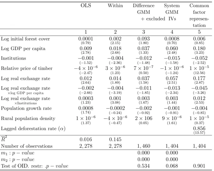
Our econometric results, using the pooling and within estimators (the latter accounts for
i) are presented in the …rst two columns of Table 3. Time dummies (to account for t) are included in both speci…cations.27 In column 3 we present the di¤erence-GMM
results using the explanatory variables lagged 3 to 5 periods in levels, plus our excluded IVs (in levels), as instruments. Column 4 corresponds to the system-GMM results where we add the equation in levels, with the …rst-di¤erenced variables, lagged 2 to 4 periods as instruments (plus the external instruments in …rst-di¤erences). Column 5 uses the same instruments as in the system-GMM estimates, while imposing the common factor restrictions.
Note that the pooling results presented in column 1 are inconsistent because they fail to account for country-speci…c heterogeneity, while the within results presented in column 2 fail to account for the correlation between the transformed initial level of forest cover and the transformed disturbance term. The GMM results (columns 3 and 4) are consistent as long as …rst-order serial correlation is absent and second-order serial correlation is present: the latter is veri…ed by our estimates (see the m2 test statistic, which is highly signi…cant,
with a p value below 0.001), whereas the former is not (see the m1 test statistic, which
rejects, again with a p value below 0.001). The overidentifying restrictions are not
26 See Hall and Mairesse (2001) and Bond, Nauges, and Windmeijer (2002), for recent surveys of the
literature on testing for unit roots in panel data.
27 For the sake of brevity we do not present the coe¢ cients associated with the time dummies in Table
rejected for the di¤erence-GMM results, whereas they are (taking a 10 percent critical level) once the e¢ ciency of estimation is increased through the addition of the equation in levels.
Taken together, these results suggest that the null-hypothesis of no serial correlation in the disturbance term of the equation in levels is untenable, which leads us to prefer the common factor restriction speci…cation presented in column 5. Here, the test of the overidentifying restrictions does not reject, and each individual common factor restriction (as given in equation (9) — all of the individual p values are above 0.900) is not rejected, though the joint test does reject. As a whole, our empirical results are relatively stable as one moves from one estimator to another (at least as far as the sign and statistical signi…cance of each individual explanatory variable is concerned), with the exception of the relative price of timber.
The main impression that emerges from the results presented in Table 3 is that the predictions of our theoretical model are not rejected by the data.
First, better institutions reduce deforestation, as predicted by Proposition 2. Though the coe¢ cient associated with the Bohn and Deacon index is not statistically signi…cant in the di¤erence-GMM and system-GMM results, it is signi…cant in the within results and in our prefered speci…cation, given by the common factor representation.
Second, the coe¢ cient associated with the real exchange rate is positive and usually statistically signi…cant (the exception being the di¤erence-GMM results), while that as-sociated with the real exchange rate times the log of GDP per capita is negative and statistically signi…cant. This con…rms the theoretical predictions of Propositions 3, 4 and 5: a real depreciation increases deforestation in poor countries, with the e¤ect be-coming negative once a threshold level of GDP per capita is reached.28 Evaluated at the
mean level of institutions in the sample, this threshold level of GDP per capita varies between a maximum of $US 1,921 using the common factor representation of column 5,
28 Note that, because of the multiplicative terms, the total marginal impact of the real exchange rate on
deforestation is given by: dzit
deit = 5+yit 6+Iit 7, which implies that the threshold level of GDP per capita
below which the impact of a depreciation on deforestation is negative is given byey = 5+ Iit 7 = 6,
to $US 909 using the within results of column 2. Clearly the threshold is operative, what-ever its precise level may be, and there is indeed a crisp separation between the behavior of deforestation with respect to depreciations in the real exchange rate in poor and rich countries.
Third, the coe¢ cient associated with institutions times the real exchange is posi-tive and often statistically signi…cant. The theoretical ambiguity of Proposition 7 is therefore resolved empirically: better institutions exacerbate the deleterious e¤ects on de-forestation of depreciations in developing countries. Using the common factor restriction results from column 5, the marginal impact of institutions on the rate of deforestation, evaluated at the mean value of the real exchange rate, is positive, though not statistically distinguishable from zero at the usual levels of con…dence.29 This brings into sharp focus
the importance of clearly separating the e¤ect of institutions into their direct e¤ect versus the e¤ect that operates through the real exchange rate.30
Fourth, the impact of the relative price of timber is unstable although, in our prefered common factor restriction speci…cation, it would appear to be the e¤ect of temporary changes in the price of timber that dominate (Proposition 6(ii)).
Fifth, increases in GDP per capita increase the rate of deforestation, ceteris paribus, while the total marginal impact of log GDP per capita on the rate of deforestation, based on the parameter estimates of column 5 and evaluated at the mean level of the real exchange rate, is not statistically signi…cant at the usual levels of con…dence.31 While this
does not con…rm Proposition 1 (deforestation is decreasing in the average rate of time preference in the population), the empirical result is not surprizing per se in that GDP
29The total marginal e¤ect of institutions on the rate of deforestation is given by dzit
dIit = 3+eit 7; where
eit is the average value of the real e¤ective exchange rate in the sample. When we include institutions,
times the real exchange rate, times log GDP per capita, the coe¢ cient associated with this variable is statistically indistinguishable from zero, and the remainder of the results are qualitatively unchanged.
30 Institutions do have a statistically signi…cant and positive marginal impact on deforestation (again,
evaluated at the mean value of the real exchange rate) when one bases inference on the within results. Their marginal impact is negative and statistically signi…cant when one uses the pooling results. For di¤erence-GMM and system-GMM, their marginal impact is not signi…cantly di¤erent from zero, as with the common factor restriction results.
31 The total marginal e¤ect of log GDP per capita on the rate of deforestation is given by dzit
dyit =
1+ eit 6. For the common factor restriction speci…cation, for example, this marginal e¤ect is equal to
per capita proxies for other e¤ects, above and beyond those associated with the rate of time preference.
Sixth, the two demographic variables (the population growth rate and rural popu-lation density) are statistically insigni…cant in all of our speci…cations, suggesting that our intuition that the impact of these variables operates through relative prices is indeed con…rmed in the data.
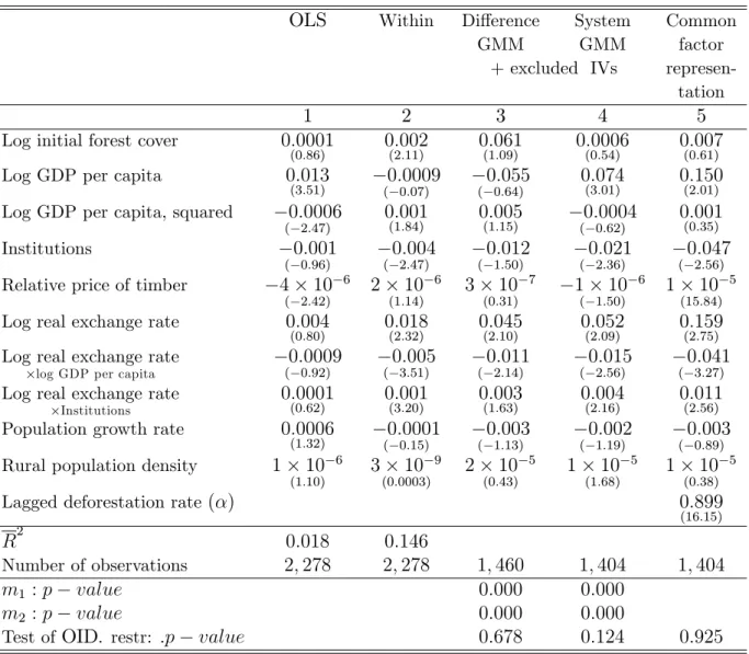
Seventh, as shown by the results presented in Table 4, there does not appear to be an environmental Kuznets curve (EKC), which would correspond to a positive coe¢ cient associated with GDP per capita and a negative coe¢ cient associated with GDP per capita squared. Indeed, the di¤erence between the pooling results in column 1 and the results reported in the four other columns of Table 4 indicate that the EKC may sometimes simply be the result of country-speci…c, time-invariant heterogeneity. This highlights the fragility of results, often reported in the literature, that purport to have identi…ed an EKC. While this issue is not the focus of this paper, it also shows how failure to account for the capital role played by relative prices can sometimes lead to misleading statistical inference. For example, if one re-estimates using the within estimator, while dropping all three variables associated with the real exchange rate, one obtains an EKC (though it has the opposite shape of what one would expect — a U instead of an inverted-U), and better institutions increase the rate of deforestation.
4
Concluding remarks
The main …nding of this paper involves the impact of the real e¤ective exchange rate on deforestation: our econometric results do not reject the null hypothesis that real depreciations increase deforestation in poor countries and decrease deforestation in rich countries. Given that real depreciations are often favored as a policy instrument in the developing world (in contrast to the developed world), this will tend to exacerbate the process of deforestation.
deforestation at the global level will be constituted by the relative rates of growth of the developing and developed worlds, and the impact that this process will have on real exchange rates. If convergence obtains, real e¤ective exchange rates will appreciate in poor countries and depreciate in rich countries, leading to a reduction in deforestation. On the other hand, an increase in inequality at the international level (divergence) will lead to a depreciation of the real e¤ective exchange rates of the developing world, leading to an increase in deforestation.
References
Angelsen, A., and D. Kaimowitz (1999): “Rethinking the Causes of Deforestation: Lessons from Economic Models,” World Bank Research Observer, 14(1), 73–98. Arellano, M. (2003): Panel Data Econometrics, Advanced Texts in Econometrics.
Ox-ford University Press, OxOx-ford, UK.
Arellano, M., and S. Bond (1991a): “Estimation of Dynamic Models with Error Components,” Journal of the American Statistical Association, 76, 598–606.
(1991b): “Some Tests of Speci…cation of Panel Data: Monte Carlo Evidence and An Application to Employment Equations,” Review of Economic Studies, 58(2), 277–297.
Arellano, M., and O. Bover (1995): “Another Look at the Instrumental Variable Estimation of Error-Components Models,” Journal of Econometrics, 68(1), 29–52. Banks, A. S. (1990): “Cross-National Time-Series Data Archive,” Center for Social
Analysis, Binghampton, NY: State University of New-York, September 1979 (up-dated 1990).
Bhattarai, M., and M. Hammig (2001): “Institutions and the Environmental Kuznets Curve for Deforestation: Crosscountry Analysis for Latin America, Africa and Asia,” World Development, 29(6), 995–1010.
(2004): “Governance, Economic Policy, and the Environmental Kuznets Curve for Natural Tropical Forests,”Environment and Development Economics, 9(3), 367– 382.
Blundell, R. W., and S. R. Bond (2000): “GMM Estimation with Persistent Panel Data: An Application to Production Functions,”Econometric Reviews, 19(3), 321– 340.
Bohn, H., and R. T. Deacon (2000): “Ownership Risk, Investment, and the Use of Natural Resources,” American Economic Review, 90(3), 526–549.
Bond, S. R. (2002): “Dynamic Panel Data Models: A Guide to Micro Data Methods and Practice,” The Institute for Fiscal Studies, Department of Economics, UCL, CEMMAP Working Paper CWP09/02, London, UK.
Bond, S. R., C. Nauges, andF. Windmeijer (2002): “Unit Roots and Identi…cation in Autoregressive Panel Data Models: A Comparison of Alternative Tests,”processed, The Institute for Fiscal Studies, Department of Economics, UCL, London, UK. Boserup, E. (1965): The Conditions of Agricultural Growth: The Economics of Agrarian
Change under Population Pressure. G. Allen and Unwin, London, UK.
Contreras-Hermosilla, A. (2000): “The Underlying Causes of Forest Decline,”Occa-sional Paper No. 30, Center for International Forestry Research, Jakarta, Indonesia. Cropper, M., and M. Griffiths (1994): “The Interaction of Population Growth and
Environmental Quality,” American Economic Review, 84(2), 250–254.
Edwards, S. (1988): Exchange Rate Misalignment in Developing Countries. The Johns Hopkins University Press, Baltimore, MD and London, UK.
(1989): Real Exchange Rates, Devaluation, and Adjustment. MIT Press, Cam-bridge, MA.
Foster, A. D., and M. Rosenzweig (2003): “Economic Growth and the Rise of Forests,” Quarterly Journal of Economics, 118(2), 601–637.
Hall, B. H., and J. Mairesse (2001): “Testing for Unit Roots in Panel Data: An Exploration Using Real and Simulated Data,” processed, University of California Berkeley.
Laffont, J.-J. (1990): The Economics of Uncertainty and Information. MIT Press, Cam-bridge, MA.
Montiel, P. J. (1999): “Determinants of the Long-Run Equilibrium Real Exchange Rate: An Analytical Model,”in Exchange Rate Misalignment. Concepts and Measurement for Developing Countries, ed. by L. E. Hinkle, and P. J. Montiel, pp. 264–290, New York, NY. Oxford University Press.
Nickell, S. J. (1981): “Biases in Dynamic Models with Fixed E¤ects,” Econometrica, 49(6), 1417–1426.
Panayotou, T. (1993): “Empirical Tests and Policy Analysis of Environmental Degra-dation at Di¤erent Stages of Economic Development,” Working Paper No 238, In-ternational Labour O¢ ce, Geneva.
Perz, S. G. (2004): “Are Agricultural Production and Forest Conservation Compati-ble? Agricultural Diversity, Agricultural Incomes and Primary Forest Cover Among Small Farm Colonists in the Amazon,” World Development, 32(6), 957–978.
Rock, M. (1996): “The Stork, the Plow, Rural Social Structure, and Tropical Deforesta-tion in Poor Countries?,” Ecological Economics, 18(2), 113–131.