HAL Id: hal-03037405
https://hal.archives-ouvertes.fr/hal-03037405
Submitted on 4 Dec 2020
HAL is a multi-disciplinary open access
archive for the deposit and dissemination of
sci-entific research documents, whether they are
pub-lished or not. The documents may come from
teaching and research institutions in France or
abroad, or from public or private research centers.
L’archive ouverte pluridisciplinaire HAL, est
destinée au dépôt et à la diffusion de documents
scientifiques de niveau recherche, publiés ou non,
émanant des établissements d’enseignement et de
recherche français ou étrangers, des laboratoires
publics ou privés.
head and neck cancer study
Pierre Fontaine, Oscar Acosta, Joël Castelli, Renaud de Crevoisier, Henning
Müller, Adrien Depeursinge
To cite this version:
Pierre Fontaine, Oscar Acosta, Joël Castelli, Renaud de Crevoisier, Henning Müller, et al.. The
importance of feature aggregation in radiomics: a head and neck cancer study. Scientific Reports,
Nature Publishing Group, 2020, 10 (1), pp.19679. �10.1038/s41598-020-76310-z�. �hal-03037405�
The importance of feature
aggregation in radiomics: a head
and neck cancer study
Pierre Fontaine
1,2*, Oscar Acosta
2, Joël Castelli
2, Renaud De Crevoisier
2, Henning Müller
1&
Adrien Depeursinge
1,3In standard radiomics studies the features extracted from clinical images are mostly quantified with simple statistics such as the average or variance per Region of Interest (ROI). Such approaches may smooth out any intra-region heterogeneity and thus hide some tumor aggressiveness that may hamper predictions. In this paper we study the importance of feature aggregation within the standard radiomics workflow, which allows to take into account intra-region variations. Feature aggregation methods transform a collection of voxel values from feature response maps (over a ROI) into one or several scalar values that are usable for statistical or machine learning algorithms. This important step has been little investigated within the radiomics workflows, so far. In this paper, we compare several aggregation methods with standard radiomics approaches in order to assess the improvements in prediction capabilities. We evaluate the performance using an aggregation function based on Bags of Visual Words (BoVW), which allows for the preservation of piece-wise homogeneous information within heterogeneous regions and compared with standard methods. The different models are compared on a cohort of 214 head and neck cancer patients coming from 4 medical centers. Radiomics features were extracted from manually delineated tumors in clinical PET-FDG and CT images were analyzed. We compared the performance of standard radiomics models, the volume of the ROI alone and the BoVW model for survival analysis. The average concordance index was estimated with a five fold cross-validation. The performance was significantly better using the BoVW model 0.627 (95% CI: 0.616–0.637) as compared to standard radiomics0.505 (95% CI: 0.499–0.511), mean-var. 0.543 (95% CI: 0.536–0.549), mean0.547 (95% CI: 0.541–0.554), var.0.530 (95% CI: 0.524–0.536) or volume 0.577 (95% CI: 0.571–0.582). We conclude that classical aggregation methods are not optimal in case of heterogeneous tumors. We also showed that the BoVW model is a better alternative to extract consistent features in the presence of lesions composed of heterogeneous tissue.
Radiomics allows quantitative analyses from radiological images with high throughput extraction to obtain prognostic patient information1.
Prediction of disease-free survival or the response to the treatment is performed via quantitative image features extracted from diagnostic or pre-treatment images. Previous improvements on radiomics workflows mainly addressed either the features optimization step, i.e. better description the tumor and its environment, or the improvement of machine learning algorithms2,3. However, some underlying relations that may exist between radiomics features and outcomes may be hidden due to the way they are quantified in the early stages of the workflow. Region-wise analysis of features is often performed by using low order statistics extracted over the entire region of the lesion. Nevertheless, additional relationships may be revealed by considering intra-regional heterogeneity using specific aggregation functions with feature maps.
The general process and related impact of feature aggregation methods has so far been little investigated in this context. In order to extract collections of scalar measurements that can be used as independent variables for statistical and machine learning algorithms4, an aggregation function is required to gather and summarize the operator responses over a considered Region Of Interest (ROI). Classical aggregation functions include first-order measures, which can be computed not only the image itself but also to response maps of image operators such as image filters or co-occurrence matrices. A common established feature aggregation method in radiomics is to
OPEN
1Institute of information Systems, University of Applied Sciences Western Switzerland (HES-SO), TechnoArk
3, 3960 Sierre, Switzerland. 2CLCC Eugene Marquis, INSERM, LTSI - UMR 1099, Univ Rennes, 35000 Rennes,
France. 3Service of Nuclear Medicine and Molecular Imaging, Lausanne University Hospital (CHUV), Lausanne,
compute the average, the variance (e.g. the first four statistical moments) or quantiles (e.g. maximum, minumum) of the distribution of the voxel values inside the ROI.
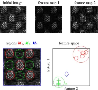
The average in particular is the most straightforward aggregation function but it is inappropriate when tumors and composing tissue are heterogeneous (i.e. non-stationary). This aspect is illustrated in Fig. 1, where the initial image (fabric) contains two visually distinct sub-regions M1 and M2 , corresponding to the visual words c1 and
c2 , respectively. The sub-regions are also distinct and well-defined in a feature space spanned by the responses
of Simoncelli wavelets5 and aggregated using the average over the sub-regions M
1 and M2 . However, when the
feature maps are aggregated over the entire image M3 , the averaging operation results in an information loss
and the resulting scalar features do not correspond to the two distinct patterns observed in the initial image (blue diamond).
In general, integrative aggregation functions such as counting or averaging over M are inappropriate for non-stationary feature maps.
Feature aggregation has been extensively studied in computer vision and led to substantial performance improvement in the context of image classification and retrieval. Most notable examples are Bags of Visual Words (BoVW)6, Fisher Vectors7, and DeepTen8. The BoVW is a well-known method in computer vision, more precisely in the field of image classification9.
It consists of describing images as a vector of visual words instead of one single scalar, where each visual word is a relatively homogeneous (stationary) region revealed via clustering (e.g. c1 and c2 in Fig. 1). Fisher Vectors
extend the BoVW framework by adding second-order moments of the features. DeepTen was introduced in the context of Convolutional Neural Networks (CNN). It is an encoding network which can be inserted between the convolutional layers and the final layer. This encoding layer learns an inherent dictionary and also affects the weights in the convolutional part during the training step.
Surprisingly, feature aggregation was little investigated in the context of radiomics. Three studies focused on the importance of feature aggregation in the context of lung cancer. Cirujeda et al.10 proposed an aggregation method based on feature covariances on top of a Riesz-wavelet decomposition, which outperformed feature aggregation based on the average. Cherezov et al.11 used clustering of a circular harmonic wavelet coefficients and showed superior categorization of cancer aggressiveness when compared to classical radiomics features. And Hou et al.12 evaluated the performance of Bag-of-features-based radiomics for differentiating ocular adnexal lymphoma and idiopathic orbital inflammation from contrast enhanced MRI. In this paper, we investigate the importance of the feature aggregation step. To this end, we compare several standard approaches (count, aver-age, variance) to the BoVW method applied to various feature types including filters and gray-level matrices (co-occurrences, run-length). The comparison is performed in the context of overall survival analysis with a multicentric cohort of head and neck cancer and PET-FDG and CT scans from 214 patients. Radiomics models were already proposed for head and neck cancer13,14, but no study focused on the impact of the aggregation function on the model performance.
Figure 1. Influence of the size and localization of the ROI M for aggregating the feature maps using the
average. Each sub-region M1 and M2 is well separated in the feature space spanned by Simoncelli wavelets and
aggregated using the average. The blue region M3 (entire image) involves the averaging of non-stationary
sub-regions. As a consequence, this blue region does not represent the true content of the image well, because its representation in the feature space (blue diamond) falls in between the true observations (red circles and green crosses). c1 and c2 represent clusters (called visual words) found using the BoVW approach allowing to reveal
and preserve pattern heterogeneity by relying on an aggregation function that is integrative regarding parts in the feature space.
This paper is organized as follows. Patient characteristics are detailed in “Patient data” section. Section “Image operators, feature maps and aggregation functions” lays the distinct fundamental elements of feature extraction by introducing image operators, their response maps (also called feature maps) and aggregation functions. The latter are further defined in the particular case of image filters and gray-level matrices (i.e. co-occurrences and run-length). Specifically considered features and their parameters are described in “Feature extraction” section. The fundamentals of the BoVW method and its specific use on with radiomics image operators are described in “Bags of visual words” section. The validation method used to estimate the performance of the proposed radiom-ics models for overall survival analysis is detailed in “Model validation” section. Corresponding results, interpre-tation and general conclusions are provided in Sections “Results” and “Discussions and conclusion”, respectively.
Material and methods
Patient data.
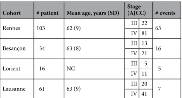
214 patients from four centers (Rennes, Lausanne, Besançon and Lorient) were retrospec-tively analyzed. The patients were aged between 18 and 75 years with an average age of 62, stage III or IV (AJCC 7th edition) with no surgery before RT, nor history of cancer, nor metastasis at diagnosis and a minimal follow-up of 3 months. All patients were treated with ChemoRadioTherapy (CRT) or RadioTherapy (RT) combined with Cetuximab. The outcome studied is dead (positive) or alive (negative) in a context of overall survival analy-sis. The study was approved by the institutional ethical committees (NCT02469922 and Commission cantonale d’éthique de la recherche sur l’être humain: CER-VD 2018-01513). Patient details are listed in Table 1.PET/CT image acquisition.
All patients underwent FDG PET/CT for staging at most 8 weeks before RT. For three centers, an injection of 4 Mbq/kg of 18F-FDG was given to the patient who fasted at least four hours. After a 60 minutes uptake period of rest, images were taken using the Discovery ST PET/CT imaging system (GE Healthcare) or the Siemens Biograph 6 True Point PET/CT scanner (Siemens Medical Solutions). First, CT (120 kV, 80 mA, 0.8 s rotation time, slice thickness 3.75 mm) was performed, followed by the PET imme-diately afterwards. A similar protocol was used for the last center; however, a smaller injection of 3.5 Mbq/kg of 18F-FDG was used with the Discovery D690 TOF PET/CT (GE Healthcare). For each patient, Gross Tumor Volume-Tumor (GTV-T) were manually segmented on each PET/CT images by the same radiation oncologist. A ROI was computed by adding a 3D margin of 5 mm to GTV-T. More details can be found in Castelli et al.15.Image operators, feature maps and aggregation functions.
In this section, we use the general theo-retic framework for radiomic analysis introduced in16 to define and isolate the role and responsibilities of the aggregation step. We consider discrete images I[k] indexed by the vector k = (k1, k2, k3) ∈Z3 . In general terms,a radiomics image analysis approach can be characterized by a set of N local operators Gn and their
correspond-ing spatial supports Gn⊂Z3 . The expression Gn{f }[k0] ∈R represents the application of the operator Gn to the
image I at location k0 and provide a scalar-valued response. The operator Gn is applied at every location k ∈ Z3 in
the image by systematically sliding its corresponding support Gn over the entire image (For the sake of simplicity,
we consider that the support of the image I is Z3 ). This process yields response maps h
n[k] (also called feature
maps) as hn[k] = Gn{I}[k] . Finally, hn[k] can be summarized over a ROI M to compute, via an aggregation
func-tion such as the average or maximum, a scalar feature ηn.
Filters. This first type of image operators considered belongs to a group of approaches called convolutional
and are based on topological operators called filters. The image operator G is fully characterized by a topologi-cal function g[k] , where G is linear and its application to the image I at the position k0 is obtained via the scalar
product of I and g as
(1) G {I}[k0] = �I[·], g[k0− ·]�.
Table 1. Patient characteristics.
Cohort # patient Mean age, years (SD) Stage (AJCC) # events
Rennes 103 62 (9) III 22 63 IV 81 Besançon 34 63 (8) III 13 16 IV 21 Lorient 16 NC III 5 5 IV 11 Lausanne 61 63 (9) III 20 7 IV 41
The full feature map is obtained via the convolution as h[k] = (g ∗ I)[k] . One classical way to aggregate the feature map h[k] to obtain a scalar valued feature η is to compute the average as η = 1
|M|
k∈Mh[k] which is integrative
and where |M| denotes the number of elements (i.e. voxels) in the region M . It is worth noting that the absolute value or the energy of the feature map must be computed for filters g[k] that are zero-mean.
Gray‑level matrices. Gray-level matrices are based on binary operators detecting the presence or absence of a
given configuration of gray-levels starting at the location k0 . These configurations can include co-occurrences17,
run-lengths18 or even size zones19. The first two are detailed below.
Gray-Level Co-occurrence Matrices (GLCM) GLCMs17 are based on a quantized image I
�[k] ∈ (1, . . . , �)
with the number of gray-levels (e.g. 8, 16, 32) and binary operators G that are detecting co-occurences between two gray levels ( i, j) observed at the position pairs k0 and k0+ k . As such, GLCMs are based on a collection
of operators defined as
This collection of responses is aggregated in an integrative fashion over M by constructing a co-occurrence matrix, which simply counts the responses of the various operators and organizes them in a square co-occurrence matrix C of dimension 2 indexed by (
i, j ). Then, a collection of scalar texture measurements η is obtained
by computing quantities (e.g., cluster prominence, correlation, entropy, also called Haralick features) from C. Gray-Level Run-Length Matrices (GLRLM) Within a quantized image I [k] , GLRLMs18 operators detect
strides of contiguous aligned voxels with identical gray-level value , length || k|| and direction k as
The aggregation is similar to GLCMs that count the response of the operators and organizes them in a run length matrix R of dimension × indexed by ( , || k|| ), where is the number of lengths || k|| considered. Collections of scalars η are computed from these matrices (e.g., short run emphasis, grey level non-uniformity, run percentage).
Feature extraction.
Before the feature extraction step, we convert CT images into Hounsfield Units (HU) and PET images into Standardized Uptake Value (SUV). We resampled images (isotropic resampling to 1mm cubic voxels) to allow adequate image scale comparisons of all texture features across image series. For step (i), from those resampled images, we extract 42 features (21 on CT and 21 on PET) and their response map from each of the 214 patients, using our own software tools that were benchmarked with the reference values provided by the Image Biomarker Standardisation Initiative (IBSI20). A list of these features is provided in Table 2. We focused on those where aggregation is critical, i.e. filters and gray-level texture matrices (also called second-order). Shape features were excluded since they do not require an aggregation step. Classical separable Wavelets (e.g. Haar, Daubechies) were not included as they are generating many irrelevant directional feature maps (e.g. XXX, XXY, XYZ, etc...), which is discussed in Section 4.6 of Depeursinge, et al.21. This is illustrated in 2D in Fig. 2. For each patient Pi we compute a collection of feature maps h[k] . Every pixel belonging to the ROI iscon-sidered as an observation in a feature space spanned by the 42 feature maps. It is worth noting that the creation of feature maps is uncommon for gray-level texture matrices. Then, we compute the gray-level matrices and related quantitative features over 5 × 5 × 5 cubic sliding windows for GLCMs and GLRLMs. In this window, we defined (2) G i, j, k{f }[k0] = 1 if f0 otherwise. [k0] = iand f [k0+ k] = j,
(3) G ,�k{I�}(k0) = 1 if a stride of gray-level starting at the position k0and ending at k0+ �kis detected,
0 otherwise.
Table 2. The list of the detailed features used in the study.
Family Feature Quantitative feature
Filter-based Laplacian of GaussianGabor Sobel
Sigma = 2mm , radius = 4mm Sigma = 11/3 , freq. = 0.4 , radius = 4 mm Kernel size = 3 × 3 × 3
Grey-level texture matrices
GLRLM Radius = 2 mm
Angles = Half of all directions (3D), symmetrical Discretization = 64 grey levels
ShortRunEmphasis LongRunEmphasis GreyLevelNonuniformity RunLengthNonuniformity LowGreyLevelRunEmphasis HighGreyLevelRunEmphasis ShortRunLowGreyLevelEmphasis ShortRunHighGreylevelEmphasis LongRunLowGreyLevelEmphasis LongRunHighGreyLevelEmphasis GLCM Radius = 2 mm
Angles = Half of all directions (3D), symmetrical Discretization = 64 grey levels
Energy InverseDifferenceMoment Entropy HaralickCorrelation ClusterShade ClusterProminence Inertia Correlation
a collection of space directions. In 3D, the number of possible spatial directions is 13 for k = 1 mm displace-ments. We also chose k = 2 mm with the same 13 directions. This resulted in a total of 26 distinct offsets and we calculated 26 corresponding GLCMs. We computed the value of the quantitative features for every voxel posi-tion k0 to generate the response maps before using an aggregation function (e.g. average) over the ROI to
com-pute scalar-valued features. The same 13 directions, radius and aggregation methodology was used for GLRLM features. This size of the sliding window was chosen as a trade-off between locality of the features (limiting the influence of surrounding objects) and the ability of the features to capture texture patterns with larger size22.
Bags of visual words.
The Bag of Visual Words (BoVW) model is an image extension of the bag of words model used in the field of information retrieval and text analysis6,23. Building a BoVW model is performed in three steps: (i) compute feature maps, (ii) reveal dictionaries of visual words using clustering and (iii) compute frequency histograms by counting occurrences of each visual word to describe an entire ROI.Then, step (ii) relies on the clustering (e.g. k-means, Gaussian mixtures, DBSCAN24) of the feature space created in step (i). Each cluster center is considered as a visual word and the set of clusters constitute the visual dictionary of our set of training images. This process is illustrated in Fig. 1 where the two clusters (i.e. visual words) c1 and c2 correspond to the two distinct texture patterns present in the initial image. We chose the Gaussian
mixture model as clustering algorithm in order to define clusters based on both mean and variance. The most interesting particularity of the BoVW method is that step (ii) acts as a feature aggregation function that is inte-grative by parts in the feature space, which allows revealing and preserving distinct homogeneous sub-regions. Step (iii) uses the results of steps (i) and (ii) to assign each voxel of the ROI to a cluster ci , thus populating a
histogram of visual words of dimension k that can be further used as a collection of scalars η for machine learn-ing models (see “Model validation” section).
Model validation.
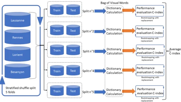
This section details the workflow used to evaluate the radiomics model’s performance using the head and neck cohort described in “Patient data” section, and in particular to test our hypothesis that feature aggregation has an important role in radiomics. To estimate the influence of the feature aggregation method on the survival prediction performance, we pooled the image data from the four centers and randomly divided it five times into a training cohort and a validation cohort using a stratified shuffling method. We used a Cox–Lasso regression model25 to predict a Hazard Score (HS) and further computed Harrell’s C-index26 as our performance measure to estimate the quality of survival analysis. We created the dictionary based on each train-ing fold. The BoVW model is compared to four other baseline models based on classical aggregation methods, as well as one univariate model based on the volume of the ROI (i.e. tumor) only27, which can be seen as the most basic aggregation function based on the count of the number of voxels inside the ROI. To summarize, we evaluate the following six models:1. Classical radiomics This model uses the classical aggregation functions described in “Image operators, feature maps and aggregation functions” section, i.e. the average for filters and the count followed by the collection of scalars for the gray-level texture matrices. Sliding-window-based feature maps are therefore not used in this case.
2. Average‑variance Average and variance inside the ROI based on the (sliding-window) feature maps computed as described in step (i) of “Feature extraction” section.
3. Average Average only inside the ROI from the feature maps, 4. Variance Variance only inside the ROI from the feature maps. 5. Volume Univariate model based on the volume of the ROI only. 6. BoVW The BoVW model as described in “Bags of visual words” section.
For all methods, the final feature collections η were standardized to z-scores using the mean and standard devia-tion estimated on the training folds.
In each fold, we evaluate the six models together by bootstrapping with replacement (1000 times) and calculat-ing the C-index. The five folds yields 5000 estimations of the C-index for each model, which we summarize with averages and their Confidence Intervals (CI) at 95%. This validation strategy is shown and summarized in Fig. 3.
Ethical approval.
All procedures performed in studies involving human participants were in accordance with the ethical standards of the institutional and/or national research committee and with the 1964 HelsinkiFigure 2. For each patient Pi , the 42 feature maps are concatenated into a matrix where each coefficient voxel of
Declaration and its later amendments or comparable ethical standards. The study was approved by the institu-tional ethical committees (NCT02469922 and Commission cantonale d’éthique de la recherche sur l’être humain: CER-VD 2018-01513).
Informed consent.
Informed consent was obtained from all individual participants included in the study.Results
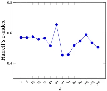
We first investigate the influence of the number of clusters k (i.e. the number of visual words) on the performance of the BoVW model. Several methods exist to determine the optimal k, including the Elbow28, Silhouette29 or Gap statistic30. In this study, we use the Gap statistic method as it is based on the measure of intra-cluster variation. Using the entire dataset, Fig. 4 reveals that k = 50 constitutes an interesting trade-off between the number of words and the ability to capture data heterogeneity. Using the validation scheme described in “Model validation” section, the influence of k on the performance of the BoVW model is shown in Fig. 5. Based on these results, we fixed k = 50 for the remaining experiments, which is also close to the dimensionality of the initial number of features extracted (i.e. 42).
Figure 6 compares the C-index values for all six models presented in “Model validation” section using the vali-dation method explained in Fig. 3. Table 3 lists the average C-index values for each method. The BoVW approach
Figure 3. Proposed validation strategy using the multi-centric cohort of head and neck cancer.
Figure 4. The number of clusters k is chosen based on the Gap value (higher is better) computed on the entire
dataset. We chose k = 50 clusters (i.e. visual words) as a very large number of cluster is required to significantly increases the Gap value beyond k = 50.
2 5 10 20 30 40 50 60 70 80 90 100 150 200 0.4 0.6 0.8
Harrell’
s
c-inde
x
k
Figure 5. Influence of k on the performance of the survival model measured using the C-index.
classical radiomic s average-v arianc e
average variance volume BoVW (k= 50) 0.5 0.6 0.7 0.8
*
*
*
*
*
Harrell’
s
C-ind
ex
Figure 6. Average C-indices and 95% CIs for the six proposed models based on various feature aggregation
methods. * p < 0.01.
Table 3. Harrell’s C-indices for the six proposed models. Mean (lower bound-upper bound) (95% CI)
Classical radiomics 0.505 (0.499–0.511) Average–variance 0.543 (0.536–0.549) Average 0.547 (0.541–0.554) Variance 0.530 (0.524–0.536) Volume 0.577 (0.571–0.582) BoVW 0.627 (0.616–0.637)
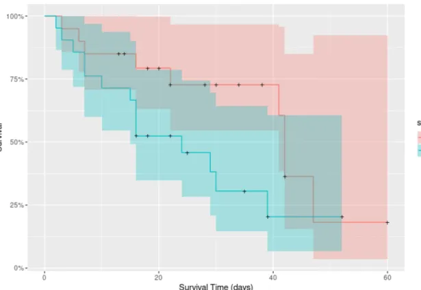
Figure 7. Kaplan–Meier curves using a risk stratification into two groups as defined by the median value of the
allows improving the performance in a statistically significant way when compared to all other aggregation methods as well as the volume. The classical radiomics model does not deliver predictions that are significantly better than random. We derived the Kaplan–Meier curve for three models (Fig. 7): Classical radiomics (Fig. 7a), Volume (Fig. 7b) and BoVW (Fig. 7c). The group stratification is based on the median of the HS provided by the prediction of the unseen test set for one train/test split: the split with a performance that was the closest to the respective observed average C-index (see Table 3) was used. The Kaplan–Meier curves (Fig. 7c) of the BoVW model suggests that the latter allows to separate the patients with distinct survival characteristics better than the other approaches.
Discussions and conclusion
Radiomics is becoming increasingly important in particular in oncology. It allows to non-invasively predict response to treatment or to characterize tumor type and aggressiveness. The main assumption of the work described in this article is that heterogeneous tumors require more advanced feature aggregation methods than the classical integrative or quantile-based methods that are commonly used in radiomics.
Averaging or using the maximum voxel value in non-stationary response maps entails the risk of mixing or discarding different sources of information.
As observed in Fig. 6 and Table 3, the method used to aggregate information inside the ROIs can significantly impact the performance of the model in overall survival analysis for head and neck cancer. The BoVW method to aggregate feature maps allowed to improve the performance of survival models with statistical significance. This result can be attributed to the fact that the BoVW relies on the integration of parts for feature aggregation, allowing to reveal and preserve sub-regions in non-stationary feature maps. Figure 6 shows that no classical feature aggregation method could outperform a simple model relying on the tumor volume solely.This can be partly explained by the large heterogeneity of our dataset with four clinical centers with different scanner manu-facturers. This generates variations in radiomics features but has a limited impact on the measure of the volume. The Kaplan–Meier analysis (Fig. 7) showed that both BoVW and volume models (Fig. 7b,c) have significant prognostic performance (i.e. p value = 0.009 and p value = 0.032, respectively), where the BoVW model allowed best stratification. By contrast, the classical radiomics model (Fig. 7a) is not significant with a p value = 0.055 (which is consistent with the observed average C-index of this model). This demonstrating the possibility of specific risk assessment in head and neck cancer, which is consistent with reported results of previous studies13–15.
This work constitutes a proof-of-concept demonstrating the importance of feature aggregation in radiom-ics studies. We recognize several limitations. First, as we focused on the feature aggregation step, the feature extraction step was not specifically optimized for the task at hand and simply relies on a classical radiomics feature set. Second, the histogram of visual words used in the BoVW is very sparse since it relies on hard cluster
assignments. Therefore, the Cox–Lasso model might struggle to work with such sparse data matrices, which we plan to further investigate in future work.
Received: 4 May 2020; Accepted: 20 October 2020
References
1. Gillies, R. J., Kinahan, P. E. & Hricak, H. Radiomics: Images are more than pictures, they are data. Radiology 278, 563–577 (2015). 2. Zhang, Y., Oikonomou, A., Wong, A., Haider, M. A. & Khalvati, F. Radiomics-based prognosis analysis for non-small cell lung
cancer. Sci. Rep. 7, 46349 (2017).
3. Parmar, C. et al. Radiomic feature clusters and prognostic signatures specific for lung and head & neck cancer. Sci. Rep. 5, 11044 (2015).
4. Depeursinge, A., Fageot, J. & Al-Kadi, O. S. Fundamentals of texture processing for biomedical image analysis: A general definition and problem formulation. In Biomedical Texture Analysis (eds Depeursinge, A. et al.) 1–27 (Elsevier, Amsterdam, 2017). 5. Portilla, J. & Simoncelli, E. P. A parametric texture model based on joint statistics of complex wavelet coefficients. Int. J. Comput.
Vis. 40, 49–70 (2000).
6. Yang, J., Jiang, Y.-G., Hauptmann, A. G. & Ngo, C.-W. Evaluating bag-of-visual-words representations in scene classification. In Proceedings of the International Workshop on Multimedia Information Retrieval 197–206 (ACM, 2007).
7. Sánchez, J., Perronnin, F., Mensink, T. & Verbeek, J. Image classification with the fisher vector: Theory and practice. Int. J. Comput. Vis. 105, 222–245 (2013).
8. Zhang, H., Xue, J. & Dana, K. Deep ten: Texture encoding network. In Proceedings of the IEEE Conference on Computer Vision and Pattern Recognition 708–717 (2017).
9. Lou, X.-W., Huang, D.-C., Fan, L.-M. & Xu, A.-J. An image classification algorithm based on bag of visual words and multi-kernel learning. J. Multimed. 9, 269 (2014).
10. Cirujeda, P. et al. A 3-D Riesz-covariance texture model for prediction of nodule recurrence in lung CT. IEEE Trans. Med. Imaging
35, 2620–2630 (2016).
11. Cherezov, D. et al. Revealing tumor habitats from texture heterogeneity analysis for classification of lung cancer malignancy and aggressiveness. Sci. Rep. 9, 4500 (2019).
12. Hou, Y. et al. Bag-of-features-based radiomics for differentiation of ocular adnexal lymphoma and idiopathic orbital inflammation from contrast-enhanced MRI. Eur. Radiol. 12 1–10 (2020).
13. Bogowicz, M. et al. Comparison of PET and CT radiomics for prediction of local tumor control in head and neck squamous cell carcinoma. Acta Oncol. 56, 1531–1536 (2017).
14. Vallières, M. et al. Radiomics strategies for risk assessment of tumour failure in head-and-neck cancer. Sci. Rep. 7, 10117 (2017). 15. Castelli, J. et al. Pet-based prognostic survival model after radiotherapy for head and neck cancer. Eur. J. Nucl. Med. Mol. Imaging
46, 638–649 (2019).
16. Depeursinge, A., Al-Kadi, O. S. & Mitchell, J. R. Biomedical Texture Analysis: Fundamentals, Tools and Challenges (Academic Press, Cambridge, 2017).
17. Haralick, R. M. et al. Textural features for image classification. IEEE Trans. Syst. Man Cybern. 6, 610–621 (1973). 18. Galloway, M. Texture classification using gray level run length. Comput. Graph. Image Process. 4, 172–179 (1975).
19. Thibault, G. et al. Texture indexes and gray level size zone matrix application to cell nuclei classification. Pattern Recogn. Inf. Process. 140–145 (2009).
20. Zwanenburg, A., Leger, S., Vallières, M., Löck, S. et al. Image biomarker standardisation initiative. arXiv preprint arXiv :1612.07003
(2016).
21. Depeursinge, A. et al. Standardised convolutional filtering for radiomics. arXiv :2006.05470 (2020).
22. Depeursinge, A. Multiscale and multidirectional biomedical texture analysis: Finding the needle in the haystack. In Biomedical Texture Analysis (eds Depeursinge, A. et al.) 29–53 (Elsevier, Amsterdam, 2017).
23. Peng, X., Wang, L., Wang, X. & Qiao, Y. Bag of visual words and fusion methods for action recognition: Comprehensive study and good practice. Comput. Vis. Image Underst. 150, 109–125 (2016).
24. Ester, M., Kriegel, H.-P., Sander, J. & Xu, X. A density-based algorithm for discovering clusters in large spatial databases with noise. In Proceedings of 2nd International Conference on Knowledge Discovery 226–231 (1996).
25. Simon, N., Friedman, J., Hastie, T. & Tibshirani, R. Regularization paths for Cox’s proportional hazards model via coordinate descent. J. Stat. Softw. 39, 1–13 (2011).
26. Harrell, F. E., Lee, K. L. & Mark, D. B. Multivariable prognostic models: Issues in developing models, evaluating assumptions and adequacy, and measuring and reducing errors. Stat. Med. 15, 361–387 (1996).
27. Dejaco, D. et al. Prognostic value of tumor volume in patients with head and neck squamous cell carcinoma treated with primary surgery. Head Neck 40, 728–739 (2018).
28. Ketchen, D. J. Jr. & Shook, C. L. The application of cluster analysis in strategic management research: An analysis and critique. Strateg. Manag. J. 17, 441–458 (1996).
29. Rousseeuw, P. J. Silhouettes: A graphical aid to the interpretation and validation of cluster analysis. J. Comput. Appl. Math. 20, 53–65 (1987).
30. Tibshirani, R., Walther, G. & Hastie, T. Estimating the number of clusters in a data set via the gap statistic. J. R. Stat. Soc. Ser. B (Stat. Methodol.) 63, 411–423 (2001).
Acknowledgements
This work was partially supported by the Swiss National Science Foundation (Grant 205320_179069) and the Swiss Personalized Health Network (IMAGINE and QA4IQI projects). The Brittany region in France provided partial funding as well.
Author contributions
P.F., H.M and A.D conceived the presented idea. J.C and R.C provided the dataset. P.F. and A.D developed the method. P.F performed the computations. P.F, A.D and O.A verified the analytical method. All authors discussed the results and contributed to the final manuscript.
Competing interests
Additional information
Correspondence and requests for materials should be addressed to P.F.
Reprints and permissions information is available at www.nature.com/reprints.
Publisher’s note Springer Nature remains neutral with regard to jurisdictional claims in published maps and
institutional affiliations.
Open Access This article is licensed under a Creative Commons Attribution 4.0 International
License, which permits use, sharing, adaptation, distribution and reproduction in any medium or format, as long as you give appropriate credit to the original author(s) and the source, provide a link to the Creative Commons licence, and indicate if changes were made. The images or other third party material in this article are included in the article’s Creative Commons licence, unless indicated otherwise in a credit line to the material. If material is not included in the article’s Creative Commons licence and your intended use is not permitted by statutory regulation or exceeds the permitted use, you will need to obtain permission directly from the copyright holder. To view a copy of this licence, visit http://creat iveco mmons .org/licen ses/by/4.0/.