HAL Id: hal-01404847
https://hal-univ-paris.archives-ouvertes.fr/hal-01404847
Submitted on 29 Nov 2016
HAL is a multi-disciplinary open access
archive for the deposit and dissemination of
sci-entific research documents, whether they are
pub-lished or not. The documents may come from
teaching and research institutions in France or
abroad, or from public or private research centers.
L’archive ouverte pluridisciplinaire HAL, est
destinée au dépôt et à la diffusion de documents
scientifiques de niveau recherche, publiés ou non,
émanant des établissements d’enseignement et de
recherche français ou étrangers, des laboratoires
publics ou privés.
interactions: Damping and finite-size effects
Jean-Baptiste Delfau, Christophe Coste, Michel Saint-Jean
To cite this version:
Jean-Baptiste Delfau, Christophe Coste, Michel Saint-Jean. Single-file diffusion of particles with
long-range interactions: Damping and finite-size effects. Physical Review E , American Physical Society
(APS), 2011, �10.1103/PhysRevE.84.011101�. �hal-01404847�
Single-file diffusion of particles with long-range interactions: Damping and finite-size effects
Jean-Baptiste Delfau, Christophe Coste, and Michel Saint JeanLaboratoire Matiere et Systemes Complexes, UMR CNRS 7057 et Universit´e Paris Diderot-Paris 7, Bˆatiment Condorcet, 10 rue Alice Domon et L´eonie Duquet, 75205 Paris Cedex 13, France
(Received 18 March 2011; published 5 July 2011)
We study the single file diffusion of a cyclic chain of particles that cannot cross each other, in a thermal bath, with long-ranged interactions and arbitrary damping. We present simulations that exhibit new behaviors specifically associated with systems of small numbers of particles and with small damping. In order to understand those results, we present an original analysis based on the decomposition of the particles’ motion in the normal modes of the chain. Our model explains all dynamic regimes observed in our simulations and provides convincing estimates of the crossover times between those regimes.
DOI:10.1103/PhysRevE.84.011101 PACS number(s): 05.40.−a, 66.10.cg, 47.57.eb I. INTRODUCTION
When Brownian particles are confined along a line in a quasi-one-dimensional channel so narrow that they cannot cross each other, anomalous diffusion appears and strongly subdiffusive behavior can be observed. This phenomenon called single-file diffusion (SFD) was first noticed in 1955 by Hodgkin and Keynes [1] who were studying water transport through molecular-sized channels in biological membranes. Since then, SFD also appeared in the diffusion of molecules in porous materials like zeolites [2–5], of charges along polymer chains [6], of ions in electrostatic traps [7], of vortices in band superconductors [8,9], and of colloids in nanosized structures [10–15] or optically generated channels [16,17]. Even though SFD can be encountered in a lot of various physical systems, most of the theoretical studies devoted to it are generally restricted to the simplest case: an infinite overdamped system with hard core interactions.
In this paper, we present simulation results concerning finite systems of long-range interacting particles. In particular, we focus on the dependency of the diffusion properties with the number of particles N and the damping coefficient γ . We exhibit new behaviors, specifically associated with systems of small numbers of particles and with small damping. In order to interpret those results, we present an original analysis based on the decomposition of the particles’ motion in the normal modes of the chain.
In the thermodynamic limit (infinite systems with finite den-sity ρ), for overdamped dynamics with hard core interactions, several analytical models [18–22] predict that at long times, the mean square displacement [MSD; see below Eq. (13)] of a particle of mass m grows as FH√twith the mobility FH given
by FH = 2 ρ ! D0 π = 2 ρ " kBT π mγ, (1)
with D0 = kBT /(mγ ) being the single-particle free diffusion
coefficient at temperature T and kB being Boltzmann’s
constant. If the interactions are long ranged, only two ana-lytical approaches have been undertaken so far [23,24], for overdamped systems in the thermodynamic limit. There it is proven that the MSD grows as FS
√
t at long times, with a mobility FSthat depends on the interaction potential, through
the isothermal compressibility κT [25] or the spring constant
K≡ ρ/κT, FS= 2 ρS(0,0) ! Deff π = 2kBT ! κ T π mγρ = 2kBT 1 √ π mγ K, (2) where S(0,0) ≡ S(q → 0,t = 0) is the long-wavelength static structure factor of the particles. The diffusivity Deff is the
effective diffusivity of a Brownian particle, taking into account its interactions with the other Brownian particles [26], and differs from the single-particle diffusivity D0. In its last
version, the expression (2) can be interpreted by considering that we can derive FSfrom FH if we replace the interparticle
distance 1/ρ by the mean square displacement kBT /K of
a particle in the potential well due to its neighbors [25]. In Appendix B, we recover the formula (2) without the assumption of overdamped Langevin dynamics (3).
In numerical simulations and experiments, the systems are obviously finite. Periodic boundary conditions are used in simulations, and annular geometries in experiments. As a consequence of finite-size effects, the asymptotic behavior at long time for the MSD is always DNt. All particles in
the system are then totally correlated and diffuse as a single effective particle of mass Nm [20]. We recover it from our analytical model and provide measurements of the diffusion coefficient DNin good agreement with this interpretation. The
SFD regime may nevertheless be observed in finite systems if the damping and the particles number are high enough, in a manner that will be clarified by our approach of finite systems dynamics.
However, most theoretical and experimental studies have been performed for overdamped systems only. This is the initial assumption in the existing models for long-range interacting particles [23,24]. The relevant experiments were generally done with solutions of colloids [10–17] for which overdamping is a safe assumption. The simulations [27,28] are shown in Ref. [25] to be in good agreement with the theoretical prediction of Kollmann, but they also assume overdamping in the choice of the simulation algorithm. In order to explore underdamped systems, we have previously studied the diffusion in a circular channel of millimetric steel balls electrically charged [25]. In this experiment, identical metallic beads are held in a plane horizontal condenser made
y x
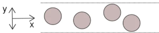
FIG. 1. (Color online) Scheme of the system.
of a silicon wafer and a glass plate covered with an optically transparent metallic layer. A constant voltage is applied to the electrodes, inducing a charge distribution of the beads. The condenser is fixed on loudspeakers excited with a white noise voltage, and we have checked that this mechanical shaking behaves as an effective thermal bath [25,29,30]. In this system the measurement of the damping constant γ proved that the balls’ diffusion is underdamped [29]. We have observed that the MSD of the particles exhibit the SFD scaling predicted for overdamped systems, with a prefactor that is only slightly higher than the theoretical prediction (2). Unfortunately, we were not able to tune the damping constant experimentally. Thus, in order to investigate the specific role of damping on the diffusion of finite systems we have developed numerical simulations that allow easy changes of the damping constant.
The paper is organized as follows. SectionII is devoted to the description of the algorithm used in our numerical simulation. In Sec.III, we present our numerical results and exhibit new behaviors specific to systems of small numbers of underdamped particles. We characterize the various regimes for the MSD scaling with time and define the crossover times between those regimes. In Sec.IV, we give a physical interpretation of those regimes in the framework of our analytical model. We recover the various scaling laws for the MSD and provide estimates of the various crossover times, showing their dependency on the damping and particle numbers. We summarize our results in Sec.V. Two appendices are devoted to complementary calculations.
II. DESCRIPTION OF THE SIMULATION A. A line of particles with long-ranged interactions We consider point particles of mass m located in the xy plane, submitted to a thermal bath at temperature T . The particles are confined by a quadratic potential in y in such a way that they cannot cross each other, as if they were diffusing in a narrow channel (see Fig.1). This lateral confinement is chosen to mimic as well as possible experimental situations. We have checked that its strength does not influence the system behavior provided the beads stay ordered.
We describe the dynamics with the Langevin equation. Let
ri = (xi,yi) be the position of the particle i. We do not take
into account the gravity, thus describing horizontal systems. The particle is submitted to a confinement force −βyiey of
stiffness β and to the interaction potential U(ri), so that the
Langevin equation reads ¨ ri+ γ ˙ri+∇U(r i) m + β myiey= µ(t) m , (3)
with γ the damping constant and µ a random force. In our simulations, the random force has the statistical properties of
a white Gaussian noise. Therefore, its components on both axes must satisfy
%µx(t)& = 0, %µy(t)& = 0, %µx(t)µy(t')& = 0, (4)
%µx(t)µx(t')& = %µy(t)µy(t')& = 2kBT mγ δ(t − t'), (5)
where %·& means statistical averaging.
It is suitable to put those equations in dimensionless form, defining the following dimensionless variables: t = #t/γ and x = #x√kBT /(mγ2). It gives us
¨#ri+ ˙#ri+ #∇#U(#ri) +
β
mγ2#yiey = #µ(#t), (6) with the dimensionless quantities
# U(#ri) = U(#ri) kBT , #µ(#t) =$ µ(#t) kBT mγ2 , (7)
and the only nonzero correlation (5) now reads
%#µx(#t)#µx(#t')& = %#µy(#t)#µy(#t')& = 2δ(#t− #t'). (8)
For the sake of simplicity, we drop the “tildes” ( #) in the rest of this section.
In order to allow a direct comparison between simulations and experiments, we take the same interaction potential as in our experimental setup [25,29,30]. It reads
U(ri) = U0 % j(=i K0 & |ri− rj| λ ' , (9)
where K0is the modified Bessel function of second order and
index 0, and λ and U0 are two constants. In principle, the
sum extends to all particles, but in practice the summation is limited to the first five neighbors of each particle, which ensures a relative precision better than 10−7 and reduces the
calculation time.
To decrease the computation time further, we re-place the Bessel functions in the expression of the force
F(ri)=−∇U(ri)=(j(=iFij(|ri−rj|)|ri −rj |ri −rj by asymptotic expressions,
Fij(x) =Uλ0 , −1x + bx + cx ln(x) -for x! 1, Fij(x) =Uλ0,$2xπe−x . 1 +a x /-for x" 1, (10) where a, b, and c are constants. They are chosen in such a way that the force and its derivative are continuous for x = 1 and that the force is equal to its actual value at this point. Those two approximations fit very well the actual force (see Fig.2).
B. Algorithm
The simulation is based on the Gillespie algorithm [31,32] that allows a consistent time discretization of the Langevin equation (6). We introduce a time step value (t, which for consistency has to be much smaller than any other characteristic time scale of the system. In dimensionless units (t = 10−3. Then the velocities ˙xi(t + (t) and ˙yi(t + (t) are
˙ xi(t + (t) = ˙xi(t) − [ ˙xi(t) + ∇U(ri(t)) · ex](t + √ 2(t µx(t), ˙ yi(t + (t) = ˙yi(t) − 1 ˙ yi(t) + β mγ2yi(t) + ∇U(ri(t)) · ey 2 (t+√2(t µy(t), (11) where ri(t) = $
xi(t)2+ yi(t)2. The positions xi(t + (t) and
yi(t + (t) of all the particles are then calculated from
xi(t + (t) = xi(t) + ˙xi(t)(t,
(12) yi(t + (t) = yi(t) + ˙yi(t)(t.
The components of the random noise µy and µx are sampled
in such a way that they have the properties given by Eqs. (4) and (8); hence they are unit normal random numbers.
We simulate systems of N particles, with periodic boundary conditions. We get from Eq. (12) N equivalent trajectories, because all beads play the same role. The system is simulated during a dimensionless time of 103, which means 106 time
steps. The quantity of interest is the MSD along the x direction, %(x2(t)& = %[x(t + t0) − x(t0) − %x(t + t0) − x(t0)&]2&, (13)
where t0 is an arbitrary initial time. The ensemble averaging
is done on every bead, since they all play an equivalent role. Moreover, the phenomenon is assumed to be stationary, so that (x2(t) do not depend on t0. For a given time t, it thus makes
sense to average on the initial time t0. Let n be the overall
number of time steps in one simulation, and nt = t/(t. Then
the averaging on the initial time t0reads
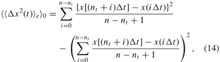
%%(x2(t)&e&0= n%−nt i=0 {x[(nt+ i)(t] − x(i(t)}2 n− nt+ 1 − 3n−n t % i=0 x[(nt+ i)(t] − x(i(t) n− nt+ 1 42 , (14) where the index i is such that t0= i(t, %·&emeans ensemble
averaging, and %·&0 means averaging on the initial time t0.
This way of averaging greatly improves the statistics when nt
is smaller than n. We use it henceforward, denoting it with the simplified notation %·& except in AppendixAwhere it is specifically discussed.
C. Orders of magnitude of the various parameters In our simulations, we work at densities ρ = 33, 100, and 533 particles per meter. The temperature and interaction strength are such that ) ranges as in the experiments in Refs. [10,16,17,25] and the numerical simulations in Refs. [27,28,33]. The interest of the simulations is to get access to parameter values that are difficult or impossible to obtain experimentally. We vary the particle number N between 32 and 1024. This last value is comparable to some simulations [27,28] but much greater than in experiments [10,16,17,25]. We vary the damping constant γ between 0.1 and 60 s−1,
extending the experimental range toward small values of γ . This is to be compared to the cutoff frequency of the chain (see Sec.IV A). With our damping constant range, we get access
to both the overdamped and the underdamped dynamics of the particles and are thus able to exhibit the subtle behaviors linked to underdamping.
We simulate the same system that was experimentally studied in Ref. [25]. In the experiments, the bead number N varies between 12 and 37, and the density ρ is 477, 566, or 654 particles per meter. The mean interparticle distance is thus such that 1.53 < 1/ρ < 2.10 mm, to be compared to the range λ= 0.48 mm of the potential. The dimensionless potential energy is such that 6 < ) < 55. The damping constant γ ranges between 10 and 30 s−1 (see Ref. [29], Fig.6). For the
experimental values of density and potential energy, the cutoff frequency ranges between 21 and 37 s−1. Experimentally, we
are thus in the underdamped regime, as was already noticed in Ref. [25].
III. SFD OF FINITE SYSTEMS: THE DIFFERENT REGIMES
In this section, we present our results about the evolution of the MSD %(x2(t)& as a function of the time t and focus on
the effects of the particle number N (at fixed density) and on the damping constant γ . Two typical examples are provided by Fig.4. The evolution of the MSD may be described by the power law %(x2(t)& ∝ tα, with an exponent α that depends
on the observation time. The interpretation detailed in Sec.IV
allows us to regroup them into three different regimes: (i) During regime I, 0! t ! τball, the MSD grows
accord-ing to H1t2.
(ii) during regime II, τball! t ! τcoll, %(x2& may be
pro-portional to Dt only, to FS
√
t only, or to Dt and then FS
√t, depending on the parameters of the simulation. The coefficient Disnot necessarily the free diffusion constant D0. When both
1 2 3 4 5 6 0 1 2 3 x Fij x λ U0
FIG. 2. (Color online) Force approximation. The thick black line represents the actual force derived from Eq. (9), the open squares and open circles are, respectively, the logarithmic and exponential approximations in Eq. (10). The two approximations are matched at x= 1.
0.1 1 10 0.01 0.1 1 10 100 time s x 2 mm 2 I II III
τball τcoll τlin
(a) 0.1 1 10 0.01 0.1 1 time s x 2 mm 2 I II III τball τcoll (b)
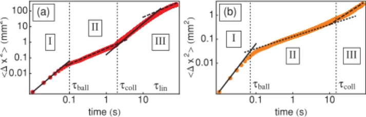
FIG. 3. (Color online) Evolution of the MSD (in mm2) according
to the time (in s) for a chain of 32 particles with density 533 m−1,
temperature T = 1012K, and interaction potential ) ≈ 7. The solid
line scales as t2, the dashed line scales as t, and the dotted line scales
as t1/2. (a) Damping constant γ = 0.1 s−1. In this low damping case,
regime II is characterized by a t scaling and regime III by a t2then a
tscaling. (b) Damping constant γ = 60 s−1. In this strong damping
case, regime II is characterized by a√tscaling and regime III by a t scaling.
scalings Dt and FS√t are observed, we define the crossover
time τsubbetween them.
(iii) A final regime, regime III, takes place for τcoll! t,
%(x2& = DNtat long times with DN (= D and DN (= D0. This
final asymptotic behavior is sometimes preceded by the scaling HNt2with HN (= H1, the crossover time being denoted as τlin.
A. The small-time regime (regime I) Regime I is defined by an evolution, %(x2& = H
1t2. It is
observed in all data displayed in Fig.4, and the prefactor H1
is independent of the damping constant [see Fig.4(a)], of the system size [see Fig.4(b)], and of the interaction potential )
0.1 1 10 0.1 0.01 1 10 100 time t s x 2 mm 2 (a) (b) (d) 0.1 1 10 80 0.01 0.1 1 10 time s x 2 mm 2 0.1 1 10 80 0.0001 0.01 1 Time t s x 2 mm 2 (c)
FIG. 4. (Color online) Plot of %(x(t)2& (in mm2) according to the
time (in s) for a density ρ = 533 m−1. Unless otherwise specified,
the parameters are N = 32, T = 1012K, ) ≈ 6.8, and γ = 10 s−1.
Specific values are as follows: (a) γ = 0.1, 1, 10, and 60 s−1 (blue
diamonds, red squares, green triangles, and orange disks, respec-tively). (b) γ = 1 s−1 and N = 4, 16, 64, and 128 (blue diamonds,
orange squares, red triangles, and green disks, respectively). (c) ) ≈ 4.4, 6.8, 9.8, and 13.4 (green disks, red squares, orange triangles, and blue diamonds, respectively). (d) T = 1010, 1011, 1012, and 1013
K, (green disks, red squares, orange triangles, and blue diamonds, respectively). The black thick line is Eq. (35), the dashed line is FS
√
twith the mobility FSgiven by Eq. (2), and the dotted line is
either DNt with DN given by Eq. (18), in (a), (c), and (d) or Dt
with D given by Eq. (16) in (b). There are no free parameters in the calculations.
[see Fig.4(c)]. In this time range (0! t ! τball), each particle
behaves independently of the others and ensures a ballistic flight at its thermal velocity √kBT /m, so that the constant
H1should thus be equal to kBT /m. The duration of this first
ballistic regime is called τball. From our data summarized in
Fig.4, we measure the constant H1and show in Fig.5(a)that
it is indeed in perfect agreement with its predicted value. This behavior is obviously not observed in the simulations of the overdamped Langevin equation [15,27,28,34], but has already been seen in simulations of the full dynamics [35,36].
B. The intermediate time regime (regime II)
If we consider now the second regime, two different behaviors with distinct power laws can be observed: Fig.4(a)
shows that for the highest values of γ , %(x2& only grows as
√
t. When γ is decreased, a linear evolution in Dt appears for τball< t < τsub. For the lowest values of γ = 1 s−1 and
γ = 0.1 s−1, the √t scaling completely disappears. This is a finite-size effect, as demonstrated by Fig. 4(b). The data displayed in this picture are recorded at a low value, γ = 1 s−1, and the√t scaling is indeed recovered at large numbers
of particles, typically N > 128. Data from simulations with 256, 512, and 1024 particles (at constant density) superimpose exactly on the data for 128 particles.
We could be tempted to explain the linear evolution in Dt by arguing that we observe the diffusion of a free particle that needs a finite time to feel the effect of confinement. If this should be the case, the diffusion coefficient D should be the diffusion constant for a free particle, which is
D0 =kBT
mγ . (15)
In Fig. 5(b), we compare our numerical values of D to D0.
It is obvious that D is very different from D0 except at the
lowest values of the density ρ (that is, low interactions). We see in Sec.IV Dthat for high interactions the coefficient D actually results from a collective behavior of the particles. In our model [see Eq. (42)], when ρ is high (high interactions), the coefficient D doesn’t depend upon γ and is given by
D=kBT 2π !κ T mρ = kBT 2π√mK. (16) In Fig. 5(c), we see that at high density the coefficient D is actually a function of kBT /
√
mK, but with a numerical coefficient that is rather equal to 1/2. The dependency of D on either the spring constant K = U''(1/ρ) or the com-pressibility κT = ρ/K indicates that collective phenomena
are responsible of this behavior and that the “free particle” hypothesis does not account for the linear behavior observed in strongly interacting systems. The modified Bessel function K0, which gives the behavior of the potential U(1/ρ) [see
(9)], is a very quickly increasing function of the density, which explains why this behavior is typical of high density systems.
When the subdiffusive regime %(x2& = F√t is observed,
as in Figs. 4(c)and Fig.4(d), we may measure the mobility F. As seen in Fig.5(d), our numerical data are in excellent agreement with the expression FSgiven in formula (2), even if
0.01 0.1 1 0.01 0.1 1 kBT m mm2s 2 H1 mm 2 s 2 (a) 0.01 0.1 1 10 0.01 0.1 1 kBT mγ mm2s 1 D mm 2 s 1 b 0.001 1 1000 106 109 1012 0.1 0.01 1 10 kBT κT 4 mρ mm2s 1 D mm 2 s 1 c 0.001 0.01 0.1 1 0.01 0.1 1 2kBT κT mγπΡ mm2s1 2 FS mm 2 s 1 2 d 0.1 0.3 1 0.1 0.3 1 kBT Nm mm2s2 HN mm 2 s 2 e 0.001 0.01 0.1 1 0.001 0.01 0.1 1 kBT Nmγ mm2s 1 DN mm 2 s 1 f
FIG. 5. (Color online) All axes are in logarithmic scales. All dotted lines are of slope 1. (a) Coefficient H1as a function of kBT /m(both in
mm2s−2). (b) Coefficient of diffusion D according to k
BT /(mγ ) [both in mm2s−1; see Eq. (15)]. The green squares represent D for systems
of low densities (ρ ≈ 100 and 33 m−1) and the purple circles represent D for systems with higher densities (ρ ≈ 533 m−1). (c) Coefficient of
diffusion D according to kBT√κT/(2√mρ) [both in mm2s−1; the numerical coefficient is slightly different from that of Eq. (16)]. The green
squares represent D for systems of low densities (ρ ≈ 100 and 33 m−1) and the purple circles represent D for systems with higher densities
(ρ ≈ 533 m−1). (d) Mobility F
Saccording to 2kBT√κT/√π mγρ[both in mm2 s1/2; see Eq. (2)]. The blue disks correspond to overdamped
systems and the red triangles to underdamped systems. (e) Coefficient HN according to kBT /(Nm) [both in mm2 s−2; see Eq. (17)]. (f)
Coefficient of diffusion DNaccording to kBT /(Nγ ) [both in mm2 s−1; see Eq. (18)].
our system is underdamped. We discuss in Sec.IV Dthe case offinite systems.
The numerical data displayed in Figs.4(c)and Fig.4(d)
are calculated for parameter values that are very close (in particular, the system sizes are equal) to the relevant parameters of the experiments reported in Ref. [25]. One can check (see Fig. 5 of Ref. [25]) that the value of the MSD is the same. The duration of the experiments is insufficient to see the final DNt scaling described in the next
section.
C. The long-time regime (regime III)
It is quite intuitive that, for very long times and finite systems, all particles become fully correlated and behave as a single effective particle of mass Nm. It is a property of
the translationally invariant mode (see Sec.IV A). For small values of γ and N, the MSD grows according to HNt2, with a
prefactor HNthat is different from the constant H1introduced
in Sec.III A. HNshould thus be given by the resolution of the
Langevin equation for a free particle of mass Nm:
HN =
kBT
N m, (17)
which is in very good agreement with our simulations as shown by Fig.5(e).
At higher values of γ , and for larger systems, we only observe a linear evolution of the MSD %(x2& = D
Ntas shown
0.05 0.25 1.25 0.05 0.1 0.15 0.2 2 γ s Τball s a 0.1 100 105 108 1011 0.05 0.075 0.1 0.1250.15 κTm ρ1 2 s Τball s b 0.1 1 10 100 700 1 10 100 700 mγ N2κ T πρ s Τcoll s c 0.5 1 2 4 8 16 1 10 100 700 N κTm ρ s Τcoll s d
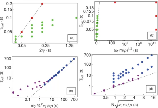
FIG. 6. (Color online) All axes are in seconds. All dashed lines are of slope 1. (a) Measures of the transition time τball according to
2/γ [log scale; see Eq. (19)]. The green circles represent τball for systems of high densities (ρ ≈ 533 m−1) and the red squares represent
τball for systems with lower densities (ρ ≈ 100 and 33 m−1). (b) Measures of the transition time τball according to √κTm/ρ[log scale; see
Eq. (20)]. The green circles represent τballfor systems of high densities (ρ ≈ 533 m−1) and the red squares represent τballfor systems with lower
densities (ρ ≈ 100 and 33 m−1). (c) Measures of the transition time τcollaccording to mγ N2κ
T/πρ[log scale; see Eq. (21)]. The blue circles
represent τcollfor systems with (N/2π)$γ2mκT/ρ >1 and the purple diamonds represent τcollfor systems with (N/2π)$γ2mκT/ρ <1 [see
Eq. (40)]. (d) Measures of the transition time τcollaccording to N√κTm/ρ[log scale; the numerical coefficient is slightly different from that
of Eq. (23)]. The blue circles represent τcollfor systems with (N/2π)$γ2mκT/ρ >1 and the purple diamonds represent τcollfor systems with
(N/2π)$γ2mκT/ρ <1 [see Eq. (40)].
resolution of the Langevin equation for a free particle of mass N m:
DN =
kBT
N mγ. (18)
This expression is in very good agreement with our results in Fig.5(f). The Fickian behavior at very long times has already been observed in numerical simulations of SFD in finite length channels [37] and is also suggested in Ref. [38].
The interpretation of Sec.IV C shows that this regime is dominated by thecollective behavior of the particles, so that we call τcollthe time at which these collective behaviors takes
place. We recover the values of DNand HNin Sec.IV Cfrom
our analytical solution (34) and give an estimate showing that the quadratic scaling is favored by small damping constants and small particle number, as is the case in Figs.4(a)and4(b).
D. Crossover times
Now that we know the evolution of %(x(t)2& in the different
regimes, we can estimate the different crossover times. In this section, we proceed heuristically, defining the crossover times by requiring continuity of the MSD for successive scalings.
Following this method, the ballistic time τball will be
the time for which the curves of equations H1t2 and 2Dt
will intersect. Depending on the expression of the diffusion coefficient D, we obtain kBT m τ 2 ball∼ 2 kBT mγ τball =⇒ τball∼ 2 γ (19) for weakly interacting systems. For strongly interacting sys-tems, one has to consider the effective diffusion coefficient D of Eq. (16), which gives
kBT m τ 2 ball∼ kBT π ! κT mρτball =⇒ τball∼ 1 π ! κTm ρ . (20) We performed measurements of τball for different values of
parameters and report them in Figs. 6(a) and 6(b). One can clearly see that two different mechanisms are at stake: the green circles that represent systems of high densities (ρ ≈ 533 m−1), which are associated with strongly interacting
particles, can be easily distinguished from the red squares that represent systems with lower densities (ρ ≈ 100 and 33 m−1),
thus weakly interacting particles. Formula (19) seems in good agreement with the transition times of weakly interacting systems, whereas formula (20) fits the values of τball for
Let us now consider τcoll. For overdamped and large
systems, it will be the time for which the curves of equation FS√tand DNtintersect, thus giving
FS√τcoll= 2DNτcoll=⇒ τcoll=
F2 4D2 N =S(0,0) 2 D20 Deff N2 πρ2 = mγ N 2κ T πρ . (21)
Note that starting from Eq. (2), using the fact that Deff =
D0/S(0,0), and introducing the length L = N/ρ of the chain,
we may recast this expression to obtain τcoll= L
2
π Deff
, (22)
which is interesting as it tells us that τcoll can be seen
as the time necessary for a given particle to diffuse over the length of the system L, with the effective diffusion coefficient that takes into account its interactions with the other particles.
In the case of small damping and small systems, the SFD behavior is not observed in the intermediate regime [see Figs. 4(a) and 4(b)], being replaced by a Dt scaling with Dgiven by Eq. (16), and the collective regime begins by a t2 evolution [see Sec.III Cand Eq. (17)]. The time τcollmay thus
be estimated by 2Dτcoll= HNτcoll2 =⇒ kBT π√mKτcoll= kBT N mτ 2 coll =⇒ τcoll= N π ! m K. (23)
One can see in Fig. 6(c) that τcoll is in very good
agreement with Eq. (21) for large values of γ N2. For
small values of γ N2, the data rather follow Eq. (23),
according to the analysis provided in Sec.IV C, particularly Eq. (38).
IV. THEORETICAL ANALYSIS
A. A chain of springs and point masses in a thermal bath In order to analyze the results presented in Sec. III, we have studied the Langevin dynamics of a chain of N beads of mass m, aligned along the x axis, interacting with a pair potential U(x), with nearest neighbor interactions. Those two simplifying assumptions are, as we will see, in excellent agreement with the actual dynamics.
Small oscillations around the equilibrium position are described by linear springs of force constant K = U''(1/ρ),
where ρ is the particle density at equilibrium [39]. Let x(l,t) be the position of particle l at time t. The equation of motion reads d2 dt2x(l,t) = −γ d dtx(l,t) + K m[x(l + 1,t) − 2x(l,t) + x(l − 1,t)] +µ(l,t) m , (24)
with the same notations as in Sec. II A. Let us consider a chain with periodic boundary conditions. We may introduce the discrete Fourier transform
X(q,t) = N % l=1 eiqlx(l,t), x(l,t) = 1 N N % k=1 e−iqklX(q k,t), (25) with qk= −π + 2πk/N for k = 1, . . . ,N. From now on, we
simplify the notations, dropping the dependency of the modes qk on the natural number k and replacing summations on k
by summations on q. The variance of the displacement x may be calculated from the Fourier modes X(q,t) as %(x2(t)& =
(
q%(X2(q,t)&/N2, with
%(X2(q,t)& ≡ %[X(q,t) − %X(q,t)&][X(−q,t) − %X(−q,t)&]&. (26) Let us first consider the mode q = 0, which will be noted simply X(t). It follows that
d2 dt2X(t) + γ d dtX(t) = µ(q = 0,t) m . (27)
Physically, this is the equation for a free particle of mass m in a thermal bath at temperature T , with damping constant γ . The solution is composed of two parts: Xd(t), which corresponds
to the deterministic motion of the particle, and the fluctuating part Xµ(t), which depends linearly on the random forcing
µ(q = 0,t). It reads X(t) − X0= X˙ 0 γ [1 − e −γ t] + 1 m 5 t 0 dt' × 5 t' 0 dt''e−γ (t'−t'')µ(q = 0,t''), (28) where X0≡ X(t = 0) and ˙X0≡ ˙X(t = 0) are the initial
con-ditions. The corresponding contribution to the MSD measured in the simulations is the double average defined by Eq. (14). It is calculated in AppendixAand reads
%(X2& = 2N kmγBT 1
t− 1 γ(1 − e
−γ t)2. (29)
The translationally invariant mode q = 0 scales as t2at small
time t ! 1/γ and then scales as t when t . 1/γ .
We now consider the modes q (= 0. Using the periodic boundary conditions x(l,t) = x(l + N,t), we see that each mode X(q,t) of wave number q (= 0 follows the equation
d2 dt2X(q,t) + γ d dtX(q,t) + 2K m (1 − cos q)X(q,t) = µ(q,t) m . (30) The roots of the characteristic polynomial associated with this equation are ω±(q) ≡ −γ 2 ± ! γ2 4 −ωq2, ω2q ≡ 2 K m(1 − cos q). (31) Physically, the mode X(q,t) behaves as a particle of mass min a harmonic potential well with pulsation ωq, forced by
0 π γ 2 ωπ q ω q
FIG. 7. (Color online) Dispersion relation ω(q) as a function of q, for q" 0 (the curve is obviously symmetric for q ! 0). The continuous line is valid for the infinite chain; the dots represent the modes for N = 32. The modes such that their frequency is less than γ /2 are overdamped; the other ones are underdamped.
the random force µ(q,t). The solution of Eq. (30) is readily obtained as X(q,t) = X˙(q,0) + ω−(q)X(q,0) ω+(q) − ω−(q) e ω+(q)t +ω+(q)X(q,0) − ˙X(q,0)ω +(q) − ω−(q) eω−(q)t+ X µ(q,t). (32)
The modes with nonzero wave number scale as kBT t2/(Nm)
at small times and saturate toward the constant value 2kBT /(Nmω2q) at very long times.
At intermediate time, the behavior of the modes q (= 0 is determined by the relative values of ωqand γ /2, as illustrated
in Fig.7.
(i) The modes such that ωq < γ /2 are overdamped. They
reach their saturation value at the time tsat∼ 1/|ω+(q)|. The
shortest saturation time is associated with q = π and reads tsatmin∼ γ /ω2πif ωπ < γ /2 or tsatmin∼ 2/γ otherwise.
(ii) The modes such that ωq> γ /2 are underdamped. They
oscillate at the frequency ω(q) ≡√ω2
q−γ2/4. Below a time which
is roughly 1/ω(π), all underdamped modes scale as t2.
We do not distinguish the overdamped (γ > 2ωq) and the
underdamped (γ < 2ωq) modes, because the final result (33) is
0.01 0.1 1 10 100 1000 0.001 0.1 10 1000 Time s x 2 mm 2
τ
ballτ
collFIG. 8. (Color online) Plot of %(x(t)2& (in mm2) according to the
time (in s), in logarithmic scale, calculated from the analytical solution (34) for a density ρ = 533 m−1, N = 32, T = 1012K, ) ≈ 6.8, and
γ= 0.1s−1. The solid line is of slope 2 and the dashed line is of slope 1. This plot is to be compared to the relevant plot in Fig.4(a). We have indicated the times τball and τcoll, respectively, given by
Eqs. (36) and (38). We see that both equations provide lower bounds for τcoll.
in both cases a real function with the same formal expression. The averaging process is explained in AppendixA. One gets
%(X2(q,t)& =2NkBT mω2q 1 1 + ω−(q)e ω+(q)t ω+(q) − ω−(q) − ω+(q)e ω−(q)t ω+(q) − ω−(q) 2 . (33)
We remark that the limit q → 0 is not singular, and by taking it properly in this expression one recovers Eq. (29). We think that it is nevertheless physically convenient to distinguish between the translationally invariant mode q = 0 and the others, because they lead to different asymptotic behaviors.
Using Eq. (33) together with Eq. (29), we obtain the MSD as %(x2(t)& = 2kBT N m 6 t γ − 1 γ2 . 1 − e−γ t/ +% q(=0 1 ω2q 1 1 + ω−e ω+t ω+− ω− − ω+eω−t ω+− ω− 2 , (34) which is the basis for the following discussion.
In the limit of very large damping, that is in the absence of the inertial term, a solution to Eq. (24) has been provided by Sj¨ogren [24]. We have thus extended his calculations to underdamped systems1and calculated the MSD in a different
way to take into account our peculiar way of averaging (14). We also extend this discussion, in the rest of this section, to the case of finite systems.
B. The ballistic regime (regime I)
Since the small-time behavior of each mode in Eq. (34) is (kBT /N m)t2, and there are N equivalent contributions to the
sum, we get
%(x2(t)&t→0∼ kBT m t
2. (35)
This result is independent of N and thus valid in the thermodynamic limit too. Because of the inertial term in the Langevin equation (24), at very small times each particle behaves independently from the others and undergoes ballistic flight at the thermal velocity √kBT /m.
In order to discuss the duration τballof this regime, let us
assume a finite, but large (in a sense to be defined later), particle number N. The time evolution of %(x2(t)& is determined by
the mode q = 0 and a summation on all modes q (= 0. All modes in the summation (34), hence the sum itself, behave as t2on a time scale such that
t ! τball≡ min 3 2 γ, 1 $ ω2π − γ2/4, γ ω2π 4 . (36)
1More precisely %(x2(t)& is equal to the correlation C(0,t) defined
by Sj¨ogren [24] and to 2W (t) introduced by Kollmann [23]. This is easily seen from the definition (13), because with the double averaging on the initial conditions and on the random noise [see AppendixAand Eqs. (28) and (32)] we get %%x(t + t0) − x(t0)&e&0= 0, and then
sta-tionarity ensures %%[x(t + t0) − x(t0)]2&& = %%[x(t) − x(0)]2&&, which
For weakly interacting or equivalently low density systems τball≈ 2/γ , which was already heuristically derived in Eq. (19)
and is shown in Fig. 6(a). For strongly interacting or equivalently high density systems, we get τball≈ 1/ωπ ∝
√
m/K ∝√mκT/ρ, in perfect agreement with our
observa-tions [Fig.6(b)] and the heuristic derivations (16) and (20). C. The collective regime (regime III)
This collective regime (regime III of Fig.3, see Sec.III C) is a property of finite systems only. This asymptotic behavior may be easily deduced from the sum (34), which is dominated by the contribution of the mode q = 0 that scales as [2kBT /(Nmγ )]t.
This corresponds to the free diffusion of a particle of mass N min a thermal bath at temperature T . At very long times, the particles are completely correlated and behave as a single particle of effective mass, the sum of all masses. The same result has been obtained in Ref. [20].
It is not difficult to estimate the time τcoll. It is the time at
which the contribution of the mode q = 0 dominates the sum of the contributions of all N − 1 other modes. Let us use the simplifying Debye approximation ω2
q = (K/m)q2. We thus get 2kBT N mγτcoll∼ % q(=0 2kBT N mω2q ∼ 2NkBT 4π2K (N−1)/2% i=1 1 i2 =⇒ τcoll∼ N2mγ 12K , (37)
where we have used the fact that the sum is the generalized harmonic number H(N−1)/2,2 which is equal to π2/6 up to
corrections of order 1/N. The fact that this time scales as N2 explains why this long time regime is seldom seen in simulations (see, however, Refs. [33] and [36]) or experiments. This is clearly illustrated by our Fig.4(b), where we show that increasing N shifts the long time regime toward longer times. This expression of τcollis equal to our previous heuristic
estimate (21). It means that the reasoning at the basis of the derivation of Eq. (37) includes in the right way the physical origin of the long-time collective behavior of the finite chain. As was already quoted in Sec.III C, at very small damping constant it is possible to observe at long times the evolution %(x2(t)& = HNt2. This is possible if the modes q (= 0 are
saturated while the mode q = 0 still evolves as [kBT /(Nm)]t2.
This requires t < 1/γ (otherwise the mode q = 0 scales as t) and that the contribution of the q (= 0 modes to the sum in Eq. (34) be less than that of the mode q = 0. Roughly speaking, we get : (x2 & t=1 γ ';<<< < q=0 ∼kBT N m & 1 γ '2 >% q(=0 2kBT N mω2q ∼ N mkBT 12K =⇒ γ2< 12K N2m, (38)
where we have used the Debye approximation to estimate the contribution of the q (= 0 modes. This means that this regime is to be observed at small damping γ and small particle number
N, which is precisely the case in Figs.4(a)and4(b). In this case, the estimate (37) should be replaced by
kBT N mτ 2 coll∼ % q(=0 2kBT N mω2q ∼ 2NkBT 4π2K (N−1)/2% i=1 1 i2 =⇒ τcoll∼ N ! m 6K. (39)
This expression of τcoll is equal to our previous heuristic
estimate (23), allowing us to interpret the t2 scaling at long
time, in systems of few particles with small damping, as a collective behavior linked to the translationally invariant mode. This regime takes place when the greatest saturation time of the mode q (= 0 is smaller than the time above which the mode q = 0 evolves as t rather than t2. The behavior
%(x2(t)& = HNt2may thus be observable when
1 ω2π/N < 1 γ =⇒ N 2π " γ2mκT ρ <1. (40) The relevance of this estimate is proved by Figs.6(c)and6(d). It also shows that the time τlinintroduced in Sec.IVis equal
to 1/γ .
D. The correlated regime (regime II)
Let us now discuss the intermediate regime2 which,
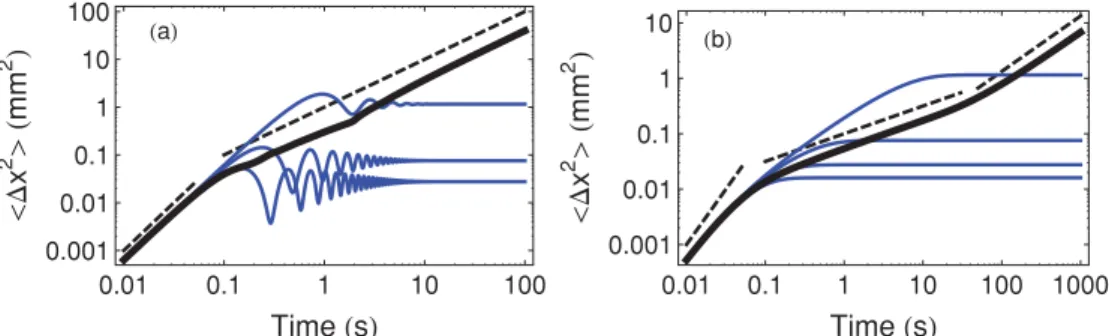
between the individual ballistic regime (regime I) and the col-lective behavior (regime III), exhibits the correlated behavior of the particles. While at asymptotically long times, all modes with finite (nonzero) wave numbers have reached a constant value, in the intermediate regime, the physical behavior of the chain at a given time t results from a subtle balance between the modes that are already saturated and those that still evolve. To simplify somewhat the discussion, we consider the limit γ / 2ω2π/N when all modes are oscillating (underdamped)
and the limit γ . 2ωπwhen all modes are overdamped.
Let us first assume a very low damping. The modes oscillate until they reach a stationary value. The time evolution of %(x2(t)& is due to the progressive disappearance of the
contributions of the first oscillation of those modes q (= 0 that have reached their maximum value. In Fig. 9(a) this is graphically illustrated with several underdamped modes (γ /2 = 0.05 s−1/ ωπ = 25 s−1), together with the complete
sum (34). As a first approximation, 1 N2 = (X2(q,t)>∼ 2kBT N mωq2 , 1 − e−γ t/2cos ω(q)t-∼kBT N mt 2. (41) At a given time t, the sum is dominated by the contributions of the modes that have not reached their first maximum, that is, those modes such that t < 1/ωq. Let n(t) be the number of
such modes. In the Debye approximation ωq = q√K/m, the
maximum wave number of those modes is 1/t√K/m so that an estimate of n(t) is given by n(t) ∼ 2(N/2π)(1/t√K/m)
2In simulations of the overdamped Langevin equation, for which
the ballistic regime cannot be seen, this intermediate regime is the first to be observed [15,27,28,34].
0.01 0.1 1 10 100 0.001 0.01 0.1 1 10 100 Time s x 2 mm 2 a 0.01 0.1 1 10 100 1000 0.001 0.01 0.1 1 10 Time s x 2 mm 2 b
FIG. 9. (Color online) Thick solid line: Plot of %(x(t)2
& (in mm2) according to the time (in s), in logarithmic scale, for a density ρ = 533 m−1,
N= 32, T = 1012K, and ) ≈ 6.8, calculated from (34) for the relevant damping constant. (a) Underdamped regime, γ = 1 s−1. The blue
(gray) curves are, from top to bottom, the modes q = π/16, q = π/4, and q = 7π/16. The dashed lines are, from left to right, of slopes 2 and 1. (b) Overdamped regime, γ = 60 s−1. The blue (gray) curves are, from top to bottom, the modes q = π/16, q = π/4, q = 7π/16, and
q= 5π/8. The dashed lines are, from left to right, of slopes 2, 1/2, and 1. (the factor 2 takes into account the modes ±|q|). The variance may thus be estimated as
%(x2(t)& ∼kBT
N mt
2n(t) ∼ kBT
π√mKt. (42) This is a normal diffusion with a diffusivity kBT /(2π
√mK) that depends on the stiffness of the interaction K, showing that it is a collective effect. This is in agreement with our observations, see Fig.5(c).
In the opposite limit of a very strong damping, all modes evolve monotonously toward their saturation value. As a first approximation, 1 N2%(X 2(q,t)& ∼ 2kBT N mωq2 6 1 +ω−ω(q)[1 − ω+(q)t] +(q) − ω−(q) ? ∼ 2kN mγBTt, (43) where we have used ω+(q) − ω−(q) ≈ γ and ω+(q) ≈ ω2q/γ
and ω−(q) ≈ −γ . A mode is saturated at a time t > γ /ω2 q.
At a given time t, in the Debye approximation, the modes that increase with time are such that q < √mγ /(Kt). This reasoning is graphically illustrated in Fig. 9(a) where we show several overdamped modes (γ /2 = 30 s−1> ωπ =
25 s−1), together with the complete sum (34). Their number
is thus n(t) ∼ 2(N/2π)√mγ /(Kt). The contributions of all such modes thus give
%(x2(t)& ∼ 2kBT N mγt n(t) ∼ 2kBT N mγt 2N 2π ! mγ Kt = 2kBT π√mKγt 1/2 =2kπBT ! κ T mργt 1/2, (44)
where we have introduced the isothermal compressibility κT
in the last expression to ease the comparison with the exact expression of FS(2). Taking into account the crudeness of our
approximations, this estimate is extremely satisfactory because we recover the SFD behavior %(x2(t)& ∝ t1/2, with a prefactor
that is almost the exact one.
In the general case, the modes with wave number q such that γ < 2ωq contribute to a t scaling of the MSD, whereas
the modes such that γ > 2ωqcontribute to the SFD behavior,
that is, a t1/2 scaling of the MSD. The typical time τ sub at
which thesubdiffusive SFD behavior takes place is thus the inverse of this cutoff frequency, τsub= 2/γ . At a given particle
number N, the minimum nonzero frequency is ω2π/N. If the
damping constant is so small that all modes are underdamped (γ < 2ω2π/N), the MSD scales as t in the collective regime II.
Increasing the damping, at fixed N, amounts to an increase in the number of overdamped modes and favors the subdiffusive t1/2 scaling for the MSD. This is exemplified by Fig. 4(a). Increasing the particle number N, at fixed γ , amounts to a decrease in the frequency ω2π/N, and hence to an increase in
the number of overdamped modes, and favors the subdiffusive t1/2scaling for the MSD. This is exemplified by Fig.4(b).
The result (44) is only approximate, so that the numerical prefactor cannot be trusted, but it explains under which conditions the SFD regime may be seen in finite systems with periodic boundary conditions [we remind the reader that this latter is the key assumption leading to Eq. (30)]. In AppendixB, we prove that the expression (2) for the mobility of long-ranged interacting systems is valid in the underdamped case γ < 2ωπ
too, in the thermodynamic limit. V. CONCLUSION
In this paper, we study the SFD of a chain of particles with long-ranged interactions, without the simplifying assumption of overdamped dynamics. We have focused our discussion on finite-size effects and the influence of low damping. We use numerical simulations of the Langevin equation with the Gillespie algorithm [31,32] and model the system as a chain of linear springs (spring constant K) and point masses (m) in a thermal bath at temperature T .
In our simulation’s data, we have identified several regimes for the time evolution of the MSD%(x(t)2&. At small times
(0! t ! τball), it evolves as %(x(t)2& = (kBT /m)t2. This is
a ballistic flight that traces back to the inertial effects and is observed whatever the damping γ or the particle number N. We recover this behavior in the thermodynamic limit (N → ∞ at finite density) from our model. The prefactor of the t2scaling
measured in our simulations is in excellent agreement with the theory.
For finite systems with periodic boundary conditions, an intermediate regime (τball! t ! τcoll) takes place. Depending
on the respective values of the damping constant and the number of particles, we may observe a diffusive behavior, a SFD behavior, or successively both. We provide a physical explanation of those observations when we express the motion of the chain in terms of normal modes of oscillations. The MSD of the chain results from the superposition of all those modes. The mode associated with the null wave number is always overdamped, and is similar to the motion of a free particle in a thermal bath, since no restoring force is exerted on it. The modes of finite (nonzero) wave numbers have the same dynamics as an oscillator in a harmonic well. At long time, the MSD of all modes with nonzero wave numbers saturates toward a constant value. The overdamped modes, which do not oscillate until they saturate, contribute to the SFD scaling %(x(t)2& ∝ t1/2. The underdamped modes oscillate
before their saturation and contribute to the linear scaling %(x(t)2& ∝ t.
In the thermodynamic limit, for systems of infinite num-ber of particles, we exhibit analytically the SFD behavior %(x(t)2& = FSt1/2 at asymptotically long times. We recover
the mobility FSthat was previously calculated for long-ranged
interactions and overdamped dynamics [23,24], thus extending the previous calculation to systems with arbitrary damping.
At asymptotically long times (t . τcoll), for a finite number
of particles with periodic boundary conditions, the system behaves as an effective particle of mass Nm. The physical origin of this behavior is the motion of the collective mode of null wave number, which is linked to the translational invariance of the system. For t" τlin" τcoll, the system
undergoes a linear diffusion with a diffusion coefficient DN =
2kBT /(Nmγ ). We show that this regime takes place whatever
the value of γ . The duration of our simulations allows us to see this regime, and the measured diffusivity is in excellent agreement with its predicted value. We provide estimates of the time τcoll∼ N2mγ /Kat large damping and τlin∼ 1/γ at
small damping. Those estimates are in good agreement with our simulation’s data. At small particle number and small damping, a new regime takes place at times τlin" t " τcoll.
It corresponds to the ballistic flight of the effective particle of mass Nm, with %(x(t)2& = (k
BT /N m)t2. In this case, the
time τcoll∼ N√m/K.
ACKNOWLEDGMENTS
We thank J. Moukhtar and F. van Wijland for helpful discussions.
APPENDIX A: AVERAGING
In this appendix, we calculate the averages used in our analysis of the simulation’s data. As explained in Sec.II B[see Eq. (14)], we perform a double averaging. The first averaging is ensemble averaging, done on the statistical distribution of the random force µ(t), and is denoted in this appendix as %·&e for the sake of clarity. This averaging is involved in
Eqs. (4), (5), and (8). The second averaging is performed on the statistical distributions of X0 and ˙X0 and is denoted as %·&
0.
It is obvious that those two averaging operations commute and that %Xµ(t)&0= Xµ(t) and %Xd(t)&e= Xd(t). In Eq. (26),
the ensemble averaging is made on the random force µ(t) so that
%(X2(q,t)&e≡ %[X(q,t) − %X(q,t)&e][X(−q,t)
− %X(−q,t)&e]&e. (A1)
1. The mode q = 0
For the translational invariant mode q = 0, all trajectories beginning at a given time t0 are equivalent, so that all
initial positions X0 are equivalent. It is easy to check that
%%X(t) − X0&e&0= %Xd(t)&0+ %Xµ(t)&e= 0. For the same
reason, the double average %%Xd(t)Xµ(t)&e&0 = 0 because
this term is linear in ˙X0 and in µ(0,t). The variance is thus
%%(X2&e&0= %%[X(t) − X0]2&e&0= %[Xd(t) − X0]2&0
+ %Xµ(t)2&e. (A2)
The variance for the deterministic part of the displacement is %%(Xd2(q,t)&e&0 = %| ˙
X0|2&0
γ2 [1 − e
−γ t]2
= N kmγB2T[1 − e−γ t]2, (A3)
where the last expression is provided by the equipartition theorem for the potential energy.
We then have to calculate the variance for the fluctuating part, %Xµ(t)2&e. We begin by calculating the following time
derivative: d dt = (Xµ2>e= d dt%Xµ(t)Xµ(t)&e = %Xµ(t) ˙Xµ(t)&e+ % ˙Xµ(t)Xµ(t)&e
= 2Re%Xµ(t) ˙Xµ(t)&e. (A4)
From Eq. (28), we get %Xµ(t) ˙Xµ(t)&e = 1 m2 t 5 0 dt' t' 5 0 dt''e−γ (t'−t'') t 5 0 dt'''e−γ (t−t''') × %µ(q = 0,t'')µ(q = 0,t''')& e. (A5)
The correlation for the random noise is %µ(l,t)µ(l',t')&e=
gδll'δ(t − t'), with g = 2mkBT γ. Besides, µ(q = 0,t) = (N l=1µ(l,t); hence %µ(q = 0,t)µ(q = 0,t')&e= N % l=1 N % l'=1 %µ(l,t)µ(l',t')&e = 2NmkBT γ δ(t − t'). (A6)
Performing the integrations in Eq. (A5), we get d dt%(X 2 µ&e= 2 N kBT mγ (1 + e −2γ t− 2e−γ t), (A7)
and a last integration gives the final result %(Xµ2&e= 2 N kBT mγ & t+1 − e −2γ t 2γ − 2 1 − e−γ t γ ' . (A8) Injecting this result and Eq. (A3) in Eq. (A2) gives the final result, Eq. (29), as stated in the text.
A. 2. The modes q "= 0
Physically, the dynamics of the mode X(q,t) with q(= 0 is identical to the motion of a damped har-monic oscillator (30). In this case, the initial values X(q,0) correspond to an initial position in a potential well and are thus not equivalent. On the other hand, the stationary state is quickly reached and the statis-tical distribution on X(q,0) is readily described taking different trajectories. In the data analysis, a trajectory is given by looking at values X(q,t + t0) − X(q,t0) and
varying the time t0 amount to varying the initial value
X(q,0). The expression (26) of the variance is thus replaced by
%%(X2(q,t)&e&0
≡ %%[X(q,t) − X(q,0) − %%X(q,t) − X(q,0)&e&0][X(−q,t)
−X(−q,0) − %%X(−q,t) − X(q,0)&e&0]&e&0, (A9)
As shown by Eq. (34), X(q,t) = Xd(q,t) + Xµ(q,t), where
Xd(q,t) is the deterministic part, linear in X(q,0) and
˙
X(q,0), and Xµ(q,t) is the random part. It is not
necessary to give explicitly the random part, all we need to know is that it is linear in the random force µ(q,t). Since %X(q,0)&0= 0, % ˙X(q,0)&0= 0, and
%Xµ(q,t)&e= 0, we have %%X(q,t) − X(q,0)&e&0= 0. The
cumbersome expression (A9) may thus be simplified to give
%%(X2(q,t)&e&0
= %%[X(q,t) − X(q,0)][X(−q,t) − X(−q,0)]&e&0
= %%X(q,t)X(−q,t)&e&0+ %%X(q,0)X(−q,0)&e&0−
−2Re[%%X(q,t)X(−q,0)&e&0]. (A10)
This may be simplified further, because the stationarity implies %%X(q,t)X(−q,t)&e&0= %%X(q,0)X(−q,0)&e&0=
N kBT /K. Moreover, since X(−q,0) does not depend on
µ we have %%X(q,t)X(−q,0)&e&0= %Xd(q,t)X(−q,0)&0.
The averaging is thus easily performed to give Eq. (33).
APPENDIX B: THE CHAIN OF SPRINGS IN THE THERMODYNAMIC LIMIT
In the thermodynamic limit N → ∞, the discrete sum in Eq. (34) may be replaced by an integral (taking advantage of the fact that the expressions for q (= 0 are valid in the limit
q → 0), %(x2(t)& = 2kBT m 1 π π 5 0 dq 1 ω2q[1 + ω−(q)eω+(q)t ω+(q) − ω−(q) − ω+(q)e ω−(q)t ω+(q) − ω−(q)], (B1) where we used the rule (1/N)(q −→ (1/2π)
@π
−π and the
invariance q → −q.
In the limit γ . 2ωπ, this integral may be expressed in
closed form [24]. This is not possible in the general case, but we may obtain its asymptotic behavior at long times using the Laplace method [40]. To this end, we express the time derivative ∂%(x2(t)& ∂t = 2kBT m 1 π π 5 0 dqe ω+(q)t− eω−(q)t ω+(q) − ω−(q). (B2) For underdamped modes, ω± = −γ /2 ± iAω2q− γ2/4, the long-time behavior is dominated by exp[−γ t/2]. Since
lim
q→0ωq = 0, the modes with small wave numbers are always
overdamped. The asymptotic behavior of the integral is dominated by the neighborhood of the maximum of ω+(q) at q = 0, with ω+(0) = 0, ω'+(0) = 0 and ω+''(0) = −2K/(mγ ). The leading term in Eq. (B2) is thus [40]
∂%(x2(t)& ∂t t→∞ ∼ 2kπ mBT 12[ 2 −tω'' +(0) ]1/21 γe ω+(0)t)(1 2) = 2[(kBT) 2 π mγ K] 1/2 1 2t1/2. (B3)
The leading behavior of the variance, at long times, is thus %(x2(t)&t→∞∼ 2(kBT Dπρ0κT)1/2t1/2. (B4) To get the last expression, we have used the relation mγ D0=
kBT and introduced the isothermal compressibility of the
chain, which is κT = ρ/K [39].
We recover the behavior for SFD of particles interacting with a long-ranged potential, as was shown by Kollmann [23] (see [25] for a rewriting of Kollmann’s result in terms of the isothermal compressibility) and Sj¨ogren [24]. Those previous calculations were done under the simplifying assumption of overdamped dynamics (γ . 2ωπ). We nevertheless recover
the same result because the asymptotics of integral (B2) is dominated by the modes of small wave numbers q / 1. Whatever the finite value of the damping constant γ , they are always overdamped because ωq→0= 0.
[1] A. Hodgkin and R. Keynes, J. Physiol.128, 61 (1955). [2] V. Gupta, S. S. Nivarthi, A. V. McCormick, and H. T. Davis,
Chem. Phys. Lett.247, 596 (1995).
[3] K. Hahn, J. K¨arger, and V. Kukla,Phys. Rev. Lett.76, 2762 (1996).
[4] T. Chou and D. Lohse,Phys. Rev. Lett.82, 3552 (1999).
[5] P. Demontis, G. Stara, and G. Suffritti,J. Chem. Phys.120, 9233 (2004).
[6] L. Wang, X. Gao, Z. Sun, and J. Feng, J. Chem. Phys.130, 184709 (2009).
[7] S. Seidelin, J. Chiaverini, R. Reichle, J. J. Bollinger, D. Leibfried, J. Britton, J. H. Wesenberg, R. B. Blakestad,
R. J. Epstein, D. B. Hume, W. M. Itano, J. D. Jost, C. Langer, R. Ozeri, N. Shiga, and D. Wineland,Phys. Rev. Lett.96, 253003 (2006).
[8] R. Besseling, R. Niggebrugge, and P. H. Kes,Phys. Rev. Lett. 82, 3144 (1999).
[9] N. Kokubo, R. Besseling, and P. Kes,Phys. Rev. B69, 064504 (2004).
[10] Q.-H. Wei, C. Bechinger, and P. Leiderer,Science 287, 625 (2000).
[11] B. Cui, H. Diamant, and B. Lin,Phys. Rev. Lett.89, 188302 (2002).
[12] B. Lin, B. Cui, J.-H. Lee, and J. Yu,Europhys. Lett.57, 724 (2002).
[13] B. Lin, M. Meron, B. Cui, S. A. Rice, and H. Diamant,Phys. Rev. Lett.94, 216001 (2005).
[14] M. K¨oppl, P. Henseler, A. Erbe, P. Nielaba, and P. Leiderer, Phys. Rev. Lett.97, 208302 (2006).
[15] P. Henseler, A. Erbe, M. K¨oppl, P. Leiderer, and P. Nielaba, e-printarXiv:0810.2302v1[cond-mat].
[16] C. Lutz, M. Kollmann, P. Leiderer, and C. Bechinger,J. Phys. Condens. Matter16, S4075 (2004).
[17] C. Lutz, M. Kollmann, and C. Bechinger,Phys. Rev. Lett.93, 026001 (2004).
[18] T. E. Harris,J. Appl. Prob.2, 323 (1965). [19] D. G. Levitt,Phys. Rev. A8, 3050 (1973).
[20] H. van Beijeren, K. W. Kehr, and R. Kutner,Phys. Rev. B28, 5711 (1983).
[21] R. Arratia,Ann. Probab.11, 362 (1983). [22] P.-G. de Gennes,J. Chem. Phys.55, 572 (1971).
[23] M. Kollmann,Phys. Rev. Lett.90, 180602 (2003).
[24] L. Sj¨ogren, “Stochastic Processes in Physics, Chemistry and Biology” (lecture notes), 2007.
[25] C. Coste, J.-B. Delfau, C. Even, and M. Saint Jean,Phys. Rev. E81, 051201 (2010).
[26] G. N¨agele,Phys. Rep.272, 215 (1996).
[27] S. Herrera-Velarde and R. Casta˜neda Priego,J. Phys. Condens. Matter19, 226215 (2007).
[28] S. Herrera-Velarde and R. Casta˜neda Priego,Phys. Rev. E77, 041407 (2008).
[29] G. Coupier, M. Saint Jean, and C. Guthmann,Phys. Rev. E73, 031112 (2006).
[30] G. Coupier, M. Saint Jean, and C. Guthmann,Europhys. Lett. 77, 60001 (2007).
[31] D. T. Gillespie,Phys. Rev. E54, 2084 (1996). [32] D. T. Gillespie,Am. J. Phys.64, 225 (1996).
[33] K. Nelissen, V. Misko, and F. Peeters,Europhys. Lett.80, 56004 (2007).
[34] P. M. Centres and S. Bustingorry, Phys. Rev. E 81, 061101 (2010).
[35] A. Taloni and M. A. Lomholt,Phys. Rev. E78, 051116 (2008). [36] D. V. Tkachenko, V. R. Misko, and F. M. Peeters,Phys. Rev. E
82, 051102 (2010).
[37] P. Nelson and S. Auerbach,J. Chem. Phys.110, 9235 (1999). [38] S. Vasenkov and J. K¨arger,Phys. Rev. E66, 052601 (2002). [39] L. Brillouin,Wave Propagation in Periodic Structures (Dover,
New York, 1953).
[40] A. Nayfeh,Introduction to Perturbation Techniques (Wiley, New York, 1993).