A data-driven reflectance model

A Data-Driven Reflectance Model

by

Wojciech Matusik

Submitted to the Department of

Electrical Engineering and Computer Science

in partial fulfillment of the requirements for the degree of

Doctor of Philosophy

at the

MASSACHUSETTS INSTITUTE OF TECHNOLOGY

September 2003

@

Massachusetts Institute of Technology. All rights reserved.

A uthor ...

...

Department of Electrical Engineering and Computer Science

August 29, 2003

Certified by

....

A e ted1 b

...

Leonard McMillan

Associate Professor of Computer Science

University of North Carolina, Chapel Hill

ilhesis Supervisor

Arthur C. Smith

Chairman, Committee on Graduate Students

Department of Electrical Engineering and Computer Science

SSACHUSETTS _INSTITUTE

-OF TECf1NOLGY

OCT 1 5 2003

BARKER

A Data-Driven Reflectance Model

by

Wojciech Matusik

Submitted to the Department of Electrical Engineering and Computer Science on August 29, 2003, in partial fulfillment of the

requirements for the degree of Doctor of Philosophy

Abstract

I present a data-driven model for isotropic bidirectional reflectance distribution functions

(BRDFs) based on acquired reflectance data. Instead of using analytic reflectance models, each BRDF is represented as a dense set of measurements. This representation allows interpolation and extrapolation in the space of acquired BRDFs to create new BRDFs. Each acquired BRDF is treated as a single high-dimensional vector taken from the space of all possible BRDFs. Both linear (subspace) and non-linear (manifold) dimensionality reduction tools are applied in an effort to discover a lower-dimensional representation that characterizes the acquired BRDFs. To complete the model, users are provided with the means for defining perceptually meaningful parametrizations that allow them to navigate in the reduced-dimension BRDF space. On the low-dimensional manifold, movement along these directions produces novel, but valid, BRDFs.

By analyzing a large collection of reflectance data, I also derive two novel reflectance

sampling procedures that require fewer total measurements than standard uniform sampling approaches. Using densely sampled measurements the general surface reflectance function is analyzed to determine the local signal variation at each point in the function's domain. Wavelet analysis is used to derive a common basis for all of the acquired reflectance func-tions, as well as a non-uniform sampling pattern that corresponds to all non-zero wavelet coefficients. Second, I show that the reflectance of an arbitrary material can be represented as a linear combination of the surface reflectance functions. Furthermore, this analysis specifies a reduced set of sampling points that permits the robust estimation of the coef-ficients of this linear combination. These procedures dramatically shorten the acquisition time for isotropic reflectance measurements.

Thesis Supervisor: Leonard McMillan

Title: Associate Professor of Computer Science University of North Carolina, Chapel Hill

Acknowledgments

I would like to express my gratitude to the following people who helped me during the last

five years at MIT.

First and foremost, I would like to thank my advisor Professor Leonard McMillan for guiding me through both the Masters and the Ph.D. programs. Not only did Professor McMillan encourage my interest in computer graphics but he has given incredible support during the key moments of my graduate studies. Professor McMillan's original thoughts and insights were the motivating force in developing these ideas. It was a great pleasure to work with him. I also would like to express my sincere thanks to Hanspeter Pfister for co-advising me on the research project that led to this thesis as well as collaborating on other research during the last three years. His enthusiasm and stimulating discussions were crucial in all of these projects. Both Professor McMillan's and Hanspeter Pfister's deep interest in the project and constant encouragement were crucial in completing the work.

I would like to thank Matt Brand for advising me on many parts of the project.

Techni-cal discussions with Matt, his algorithms, and his research code were essential in develop-ing this data-driven reflectance model.

I also would like to express my gratitude to my thesis committee members Professors

Fredo Durand and Ted Adelson for their time and their valuable input on the draft of this dissertation. Discussions with Professors Fredo Durand, Steven Gortler, Julie Dorsey, and Markus Gross during various stages of the project were enormously helpful.

Thanks also go to Henrik Wann Jensen for his assistance with his Dali renderer, Paul Lalonde for his wavelet shader, Paul Debevec for the light probes, and Matt Peters for the intial data analysis. I wish to thank Joe Marks for the continual support of this project and for hosting it at MERL. Also, my thanks go to Barb Cutler, Ray Jones, and Addy Ngan for providing me with constructive feedback on the drafts of the dissertation. In addition, I would like to thank the whole Computer Graphics Group at MIT for their support.

Finally, my deepest gratitude goes to my family. I would like to thank my parents and my wife Gosia for their love, patience and encouragement throughout the years.

Contents

1 Introduction

1.1 Thesis O verview . . . .

2 Previous Work

2.1 Radiometry and Reflectance . . . . 2.1.1 Radiometry . . . .

2.1.2 Reflectance . . . .

2.1.3 Properties of BRDFs .

2.2 Analytic Reflectance Models . . . .

2.2.1 Phenomenological Models

2.2.2 Physically Based Models .

2.3 Reflectance Measurement . . . . 2.4 Reflectance Representations . . . .

2.5 Dimensionality Reduction Methods

2.5.1 Linear Methods . . . .

2.5.2 Non-linear Methods . . . . 2.6 Summary . . . .

3 Measurement and Data Representation 3.1 Measurement System . . . .

3.2 Geometric Calibration . . . .

3.3

3.4

High-Dynamic Range Radiance Measurements BRDF Computation . . . . . . . . 1 5 . . . . 1 6 . . . . . . 1 9 . . . . 20 . . . . 2 1 . . . . 23 . . . 25 . . . . 27 . . . . 27 . . . . 28 . . . . 3 2 . . . . 40 41 41 44 44 45 9 13 14 14

3.5 Alternative BRDF Computation . . . 46

3.6 Data Representation . . . .. 47

3.7 Comparison with Analytic Reflectance Models . . . . 50

3.8 Summary . . . 52

4 Model Construction 54 4.1 Analysis Using PCA . . . . 55

4.2 Analysis Using Other Linear Methods . . . . 59

4.2.1 Analysis Using Non-negative Matrix Factorization . . . . 59

4.2.2 Analysis Using Multidimensional Scaling . . . . 60

4.3 Limitations of the Linear Model . . . . 61

4.4 Non-linear Dimensionality Reduction . . . . 62

4.5 Obtaining More Data Points . . . . 65

4.5.1 Efficient Measurement . . . . 66

4.5.2 BRDF Hallucination . . . . 66

4.6 Discussion . . . 66

5 User-Defined Parameterization 68 5.1 Trait Vectors Specification . . . . 69

5.1.1 Mean Difference . . . . 69

5.1.2 Fisher's Linear Discriminant . . . . 70

5.1.3 Support Vector Machines . . . . 71

5.2 Enforcing Physical Validity of the Data-Driven Model . . . . 72

5.3 Modelling Results . . . . . . . .. . 73

5.4 Representing Physical Processes . . . .. 79

5.5 Discussion . . . .. . . . . . .. . . . . . 81

6 Efficient Storage and Measurement 82 6.1 Wavelets and Discrete Wavelet Transform . . . . 82

6.2 Wavelet Representation of BRDFs . . . . 84

6.4 Pull-Push Reconstruction of BRDFs . . . . 88

6.5 Linear Combinations of BRDFs . . . . 90

6.6 Reconstruction Results . . . 92

6.7 Summary . . . . 95

7 Conclusions and Future Work 96 7.1 Conclusions . . . . 96

7.2 Extensions and Future Work . . . . 98

7.2.1 Analysis of Other Surface Reflectance Functions . . . . 98

7.2.2 Real-Time Rendering . . . . 99

7.2.3 Inverse Methods . . . 100

A Rendering 102 A. 1 Simple Direct Illumination . . . 103

A.2 Monte Carlo Path Tracing . . . 103

A.2.1 Basic Monte Carlo Integration . . . 105

A.2.2 Sampling Random Variables . . . 106

A.2.3 Uniform Sampling . . . 106

A.2.4 Importance Sampling . . . 107

A.3 Rendering Using Wavelet-Compressed BRDFs . . . 110

List of Figures

2-1 Radiance Definition. . . . . 16

2-2 Geometry of BSSRDF. . . . . 17

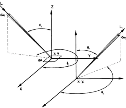
2-3 Geom etry of BRDF. . . . . 18

2-4 A simple charting example. . . . . 37

3-1 A photograph of my high-speed BRDF measurement gantry. . . . 42

3-2 A schematic of my high-speed BRDF measurement gantry. . . . 42

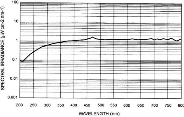
3-3 Spectral Irradiance 50 cm from the light source. . . . 43

3-4 Geometric construction used to compute mapping between BRDF coordi-nates and sampling rays. . . . .. 47

3-5 The standard and changed coordinate frame. . . . . 48

3-6 Two log images of a sphere. . . . .. 49

3-7 Pictures of 100 of the acquired materials. . . . . 49

3-8 Comparison between analytic models and measured reflectance. . . . . 51

3-9 Rendered teapots using BRDFs from my database. . . . . 53

4-1 Plot of the eigenvalues and the reconstruction error. . . . 57

4-2 The mean and the first 11 principal components. . . . . 57

4-3 Reconstruction of different BRDFs from principal components. . . . . 58

4-4 "Manufacturing" a material with a BRDF equivalent to any convex combi-nation of the source BRDFs. . . . . 62

4-5 Convex combinations that correspond to unlikely BRDFs. . . . . 63

4-6 Data reconstruction error as a function of the dimensionality of the global chart. ... ... .. 64

4-7 Non-linear spaces generate valid BRDFs where linear spaces fail.

5-1 A trait defined using mean difference. . . . .

5-2 Diffuseness trait vs specularness trait... 5-3 Metallic-like trait vs specularness trait. 5-4 Glossiness trait vs diffuseness trait. . . . 5-5 Navigation in the linear space. . . . .

5-6 Navigation on the non-linear manifold. . . . .

5-7 Progression of the steel oxidation process. . .

5-8 Rust formation. . . . .

6-1 Comparison of BRDFs expressed in common densely sampled BRDFs. . . . . . . . . 74 . . . . 75 . . . . 75 . . . . 76 . . . . 77 . . . . 78 . . . . 79 . . . . 80

wavelet basis with original . . . . 93 6-2 Comparison of wavelet reconstructed BRDFs using 69,000 sparse samples

with the original densely sampled BRDFs. . . . .

6-3 Comparison of pull-push reconstructed BRDFs using 69,000 sparse sam-ples with the original densely sampled BRDFs. . . . . 6-4 Comparison of BRDFs reconstructed as linear combinations of original

BRDFs using 800 samples with original densely sampled BRDFs. . . . . .

A-

1

Renderings using direct illumination. . . . .

A-2 Renderings under complex natural illumination. . . . . 93 94 94 104 109 65

Chapter

1

Introduction

Modeling and measuring how

light

is reflected from surfaces is a central theme in both computer graphics and computer vision. The Bidirectional Reflectance Distribution Func-tion (BRDF) describes reflectance under the assumpFunc-tion that all light transport occurs at a single surface point'. A general BRDF describes reflected light as a four-dimensional function of incident and exitant directions. This thesis focuses on the important subclass of

isotropic BRDFs, for which rotations about the surface normal can be ignored. Isotropic

BRDFs are functions of only three angles (the incident illuminations angle relative to the surface normal and two angles to parameterize the reflected radiance).

Traditionally, physically inspired analytic reflectance models [7, 17, 39] or empirical reflectance models [41, 55, 25] provide the BRDFs used in computer graphics and com-puter vision. These BRDF models are only approximations of reflectance of real materials. Furthermore, most analytic reflectance models are usually limited to describing only partic-ular subclasses of materials - a given reflectance model can represent only the phenomena for which it is designed. The models have evolved over the years to become more complex, incorporating more and more of the underlying physics. It is worth to note that many of the physically based models are based on material parameters that in principle could be measured, but in practice are difficult to acquire.

An alternative to directly measuring model parameters is to directly measure values of

'While the original definition of BRDF [37] also describes some limited subsurface scattering effects, the light interaction at a single surface point is commonly accepted in the literature.

the BRDF for different combinations of the incoming and outgoing angles and then fit the measured data to a selected analytic model using various optimization techniques [55, 57, 25, 44]. There are several shortcomings to this measure-and-fit approach. First, a BRDF represented by an analytic function is only an approximation of real reflectance - measured values of the BRDF are usually not exactly equal to the values of the analytic model. The measure-and-fit approach is often justified by assuming that there is an inherent noise in the measurement process and that the fitting process filters out these errors. This point of view, however, ignores more significant modelling errors due to approximations made by the analytic reflectance model. Many of the salient and distinctive aspects of a material reflectance properties might lie within the range of these modelling errors. Second, the choice of the error function with which the optimization should be performed is not ob-vious. For example, error based on the Euclidean distance is a poor metric since it tends to overemphasize the importance of the specular peaks and ignore the off-specular reflec-tion properties. Finally, there is no guarantee that the optimizareflec-tion process will yield the best model. Since most BRDF models are highly non-linear, the optimization framework used in the fitting process relies heavily on the initial guess for the model parameters. The quality of the initial guess can have a dramatic impact on the final parameter values of the model.

The third approach to modelling reflectance is to acquire dense measurements of re-flectance and use these tabulated measurements directly as a BRDF. This approach pre-serves those subtleties of the reflectance function that are lost in a data-fitting approach. The classical device for measuring BRDFs is the gonio-reflectometer [8, 10, 38], which is composed of a photometer and light source that are moved relative to a surface sample under computer control. By design, such devices measure a single radiance value at a time, making this process very time-consuming. There have been efforts to make this acquisition process more efficient by measuring many BRDF samples at once. This can be achieved

by using a digital camera and mirrors [55, 11] or spherical samples of the measured

ma-terial [34]. The approach of using tabulated BRDFs becomes even more expensive if the reflectance for all materials in a scene needs to be measured and stored. Furthermore, one ends up with a collection of measured BRDFs and not with a parameterized reflectance

model. Any change to the material property would require finding a real material with the desired property and acquiring its reflectance.

I propose another alternative - a data-driven approach for modelling surface reflectance.

I capitalize on the fact that it is feasible to rapidly acquire accurate reflectance

measure-ments. I acquire BRDFs for a large representative set of materials. Materials in my col-lection include metals, paints, fabrics, minerals, synthetics, organic materials, and others.

I introduce a new approach to BRDF modelling, an approach that is data driven - it in-terpolates and extrapolates new BRDFs from the representative BRDF data. My approach has the advantage that the produced BRDFs look very realistic since they are based on the measured BRDFs. Furthermore, I provide a set of intuitive parameters that allow users to change the properties of the synthesized BRDF. I also let users create their own parame-ters by labelling a few representative BRDFs. I believe that this way of specifying model parameters makes my model much easier to use and control than the analytic models in

which the meaning of parameters is often non-intuitive [40].

In my data-driven model, it is undesirable to store all acquired BRDFs explicitly. This leads me to the analysis of the space of all possible BRDFs for common materials in the world. A BRDF for these materials is not an arbitrary function, and I seek a representation for all possible functions corresponding to physical BRDFs. I treat each of my acquired BRDFs as a single high-dimensional vector where each measurement is an element of this vector. Then I apply both linear and non-linear dimensionality reduction tools to obtain a low dimensional manifold along with its linear embedding space that characterizes the set of BRDFs I measured. In the process I also obtain a backprojection operator that maps the embedding space of the manifold to the original BRDF space. Therefore, I can always compute the corresponding BRDF for each point on the manifold. An interesting side effect of my approach is that it suggests an inherent dimensionality for the space of all isotropic BRDFs.

The measurement and analysis of a relatively large collection of densely sampled isotropic BRDFs from many different materials also lead to more efficient measurement procedures of reflectance functions. I observe that sampling BRDF uniformly is very inefficient since it requires a huge amount of measurements. For example, an angular resolution of 0.5

requires more than 46 million measurements. Therefore, I start by answering the question, "What is the required sampling frequency over the domain of the isotropic BRDF to ad-equately measure it?" The first proposed measurement procedure is based on the wavelet analysis of the space of measured BRDFs. I observe that the BRDFs in my dataset have varying frequency content at various points in their domain. For example, specular high-lights have complicated local spectrums that contain high frequencies, whereas off-specular signals are typically smooth with simple local spectrums. I exploit these properties of BRDF spectrums to derive an efficient measurement procedure that employs a non-uniform sampling of the reflectance function. The sampling density at each point of the function domain is a function of the signal frequency that adequately represents any BRDF.

The linear reflectance model leads to another efficient measurement procedure. I note that the set of the basis functions generated by the linear model is the optimal basis to repre-sent the BRDFs in the original dataset. Furthermore, I show that new isotropic BRDFs (not in the original set) can also be represented as linear combinations of these basis functions or as linear combinations of the BRDFs in the original set. This implies that one needs to make very few measurements, just enough to constrain the few parameters of the linear model, in order to obtain the densely sampled representation of any new BRDF.

To summarize, the central thesis of my dissertation can be expressed in the following statement:

Reflectance of materials in nature can be modelled as a linear combination of a small set of basis functions derivedfrom analyzing a large number of densely sampled reflectance functions of different materials.

In more detail, the main contributions of my thesis are as follows:

" I introduce the first data-driven reflectance model.

" I introduce a set of perceptually-based parameters for this model. I also let users

create their own parameters.

* I analyze both linear and non-linear dimensionality of the space of isotropic BRDFs.

materials I have measured. Using my model I can also generate difficult to represent effects such as rust, oxidation, or dust.

* I demonstrate two novel BRDF sampling procedures. The procedures require few measurements and reconstruct dense BRDF representation to within measurement er-ror. The first procedure is based on the wavelet analysis of BRDFs in my dataset. The second procedure follows directly from subspace analysis of BRDFs in my dataset.

1.1

Thesis Overview

The rest of my thesis is organized as follows: In the second chapter I present background material about reflectance and describe the most significant previous work in the reflectance modelling and representations. I also outline linear and non-linear dimensionality reduction techniques that are used to construct my data-driven reflectance model. In the third chapter I describe the measurement system and procedure that are needed to obtain densely sampled, tabulated BRDFs for a large collection of different materials. In chapter 4, 1 present the linear and non-linear analysis of my BRDF dataset. Chapter 5 contains the description of the methods used to create user-defined, perceptual parameterizations for my data-driven model. The subject of chapter 6 is efficient measurement and storage; I show how to represent the data-driven reflectance model using wavelets. The wavelet representation and the linear analysis of chapter 4 lead to the efficient and simple measurement procedures. These procedures allow us to measure BRDFs using much fewer samples than standard procedures. Finally, chapter 8 summarizes the results and discusses directions for future work.

Chapter 2

Previous Work

There has been a great deal of research on how light reflects from surfaces. Many different aspects of reflectance have been examined. In this chapter, I will first describe a nomen-clature for reflectance - reflectance can be expressed in various ways depending on the assumptions one is willing to make. Next, I describe how reflectance has been approxi-mated using analytic formulas. The third section explains how reflectance of real-world surfaces has been measured in previous research. Next, I describe different representations for surface reflectance.

The second part of this chapter is devoted to dimensionality reduction techniques. I start with linear (subspace) methods that have been used for some time. Then, I move on to the recently developed non-linear (manifold) methods. These methods are an essential part of this thesis since I use them to derive my data-driven reflectance model.

2.1

Radiometry and Reflectance

Radiometry is the measurement of the electromagnetic radiation in the ultraviolet, the visi-ble, and the infrared frequency spectrum. I will define the most important radiometric terms and then use them to describe the reflection of light from materials. I define reflectance as the ratio of the reflected light to the incident light at the surface. I consider the most general model of surface reflectance and explain the various simplifications and assumptions that lead to an isotropic BRDF model.

2.1.1

Radiometry

In this section I introduce the most important radiometric terminology and quantities. The descriptions follow the concepts defined in Nicodemus et al. [37], Jensen [18], and Marschner [32].

Radiation Flux

Radiation flux (or radiant flux, electromagnetic flux), usually denoted with 0D, is equivalent to power. It measures the time-rate flow of light energy:

(D dQ (2.1)

dt

where

Q

denotes the energy of a collection of photons across all wavelengths and t denotes time. The unit of flux is the Watt [W].

Radiance

This is the most fundamental concept in radiometry. It is a physical quantity equivalent to the psychological concept of brightness observed by humans. It is usually denoted with the letter L and defined for all directions ol. It measures electromagnetic flux dcD travelling in the small range of directions through the solid angle element dO and crossing an element of projected area dA (see Figure 2-1):

d4D

L(w) dD (2.2)

cos~d Ad o

The unit of radiance is Watt [

meter2 .steradian m -sr

Irradiance

This quantity, denoted with the letter E, measures the differential incident flux falling onto a differential area of a surface. It is defined for all directions o:

d'D

dE(w) d (2.3)

dA

Z

L

da

X

Figure 2-1: Radiance (L) measures electromagnetic flux d(D travelling in the small range

of directions through the solid angle element do and crossing an element ofprojected area dA

Irradiance can be seen as a density of the incident flux falling onto a surface. It can be also obtained by integrating the radiance over the solid angle. The unit of irradiance is

Watt

_[Wi

meter M

2.1.2

Reflectance

Nicodemus et al. [37] defines reflection as the process by which electromagnetic flux in-cident on a stationary surface leaves the surface without a change in frequency. The re-flectance is the fraction of the incident flux that is reflected. Phenomena like transmission, absorption, spectral effects, polarization, and fluorescence are not considered in this thesis.

I consider the reflectance under the assumption of simple ray optics - the light travels only along the straight lines. Therefore, phenomena explained by wave optics (interference, diffraction) are also not considered.

z E), dA

x

dxy Y Xr Y,

Figure 2-2: BSSRDF S, is defined as a ratio of reflected radiance dL in the direction

(Or,

Or) at a point (xr,yr) to incident flux d4bi coming from direction

(0j,

pi)

at a point (xi,yi).

BSSRDF

BSSRDF is a very general model of light transport. It considers all potential paths for the radiance seen emerging from a surface. Let's assume that the light reaches the material surface. Some fraction of it is absorbed and changed into heat. Some of the light is imme-diately reflected back in different directions. The rest scatters inside the material and some portion may exit the surface at different points. The material sample is not assumed to be homogenous; thus, each point on the surface might reflect the light in a different way. The function that describes how light reflects from a given surface is called the bidirectional scattering-surface reflectance distribution function (BSSRDF) [37], typically denoted with

S. BSSRDF is a function of 8 variables. It is defined as a ratio of reflected radiance dLr in

the direction (Or, Or) at a point (xr,yr) to incident flux d<Di coming from direction (0i, $j) at a point (xi,yi) (see Figure 2-2):

dLr(Or,

#r,xr,yr)

L IL

z

d, _do,

CdLA _Y

X

Figure 2-3: BRDE

f,.,

is defined as a ratio of incoming irradiance dEi(1&i, OPs) to the outgo-ing radiance dL,(r, 0Pr).

The unit of BSSRDF is m [ meter 2 .steradian I m2 -. sr

BRDF

One of the most useful models of reflectance is Bidirectional Reflectance Distribution Function (BRDF), denoted with

fr.

It deals with the light that is immediately reflected when reaching the surface (the light that scatters inside the material and then leaves is not considered). This simplification of the BSSRDF takes advantage of the observation that, for most materials, the radiant flux incident at a point emerges from a point very near the point of incidence. This model of reflectance assumes that the surface is homogenous. BRDF is a function of four variables: two variables specify the incoming light direction, two other variables specify the outgoing light direction. It is defined as a ratio of incoming irradiance dEi(6i, $i) to the outgoing radiance dLr(Or, 'r) _{(see Figure 2-3):}

(2.5)

fr (i,'iOr, 'Pr) = dLr(Or,Or) dLr(Or, r)

The unit of BRDF is sterdian

Isotropic BRDF

Isotropic BRDFs are an important subclass of BRDFs. The isotropic model is valid for materials for which rotations about the surface normal can be ignored. (The reflectance is the same when the material sample is rotated about the normal while the directions of the incoming irradiance and outgoing radiance are fixed.) In this case BRDF can be written as a function of only three variables. The variables or and $i can be replaced by one variable

Odiff (or -Oi). Therefore, the expression for isotropic BRDF can be expressed as follows: dLr(&r, Odiff) dLr(Or, Odiff)

fr(Oi, &r,Pif dO6i,'Pd.f) _{dEi (0i, Odiff) Li (0i, Odiff) cos Oi d wr} (2.6)

However, anisotropic surfaces - surfaces with preferred directions - cannot be modelled using isotropic BRDFs that are parameterized using only three angles. Anisotropic surfaces include brushed or burnished metals, hair, and fur. Kajija [21] gives as an example cloth that is composed of a weave of threads. Light which strikes threads along their length scatters differently than when it strikes them perpendicularly. Anisotropic surfaces have microgeometry with strongly oriented elements. The orientation of these elements causes the light to reflect in preferred directions relative to the local coordinate system expressed

by the tangent, normal, and binormal. A distant observer does not see the microstructure,

but instead only its effect on the reflected light. However, for the vast majority of the natural and man-made surfaces the microgeometry is randomly distributed and does not have any preferred direction.

2.1.3

Properties of BRDFs

BRDFs are not arbitrary functions. In order to obey the basic principles of physics they must satisfy certain constraints. I will describe the most important of these properties.

Non-negativity

All values of function fr must be non-negative. In fact, they can be any value from the

Energy Conservation

The energy conservation property can be stated in the following way:

Jfr (0i, i, Or, Or) dp (Or, Or) < 1 for all (i, 1 0). (2.7)

This property means that the amount of energy that is received by the surface element from some specific direction must be greater than the sum of the energy emitted by the surface element in all possible directions. This must be true for the energy received from all possible directions. The underlying assumption is that the surface element does not emit the energy by itself (e.g., the surface is not fluorescent).

Reciprocity

This property is also called Helmholtz's law of reciprocity. It states that the surface re-flectance should be independent of the direction of the light flow - if the flow of light is reversed the value of the BRDF should be the same. This means that swapping the incom-ing and outgoincom-ing directions should yield the same value of fr

fr(i, i, 6r, Or) = fr(Or, Or, i, 0i). (2.8)

Veach [54] has a detailed discussion of the reciprocity. He argues that reciprocity cannot be derived from the second law of thermodynamics or from the principle of time reversal invariance. However, reciprocity is widely observed and commonly assumed in reflection modelling.

2.2

Analytic Reflectance Models

Traditionally, in both the fields of computer graphics and computer vision, surface re-flectance has been approximated with analytic rere-flectance models with varying degrees of complexity. These analytic reflectance models can be divided into two groups. (1) Phe-nomenological models - models that approximate the reflectance without analyzing under-lying principles of physics. Phenomenological models are "ad hoc" empirical formulas that attempt to reproduce the typical reflectance properties seen in real surfaces. (2) Physically

based models - these models try to make some simplifying assumptions about underlying physical properties of the surface. Physically based models usually model some specific phenomenon or specific types of materials (e.g., conductors).

2.2.1

Phenomenological Models

The phenomenological models initially used a simple cosine lobe [41] to approximate re-flectance. They were modified to be physically plausible and more general [25]. Alter-natively, a Gaussian instead of a cosine lobe has been used [55]. I will describe three phenomenological models that are commonly used in computer graphics.

Phong Model

The Phong model [41] is the most widespread reflectance model used in computer graphics. The original Phong model is not physically plausible - it does not satisfy energy conserva-tion or reciprocity; however, there are simple modificaconserva-tions that ensure that these properties are met. The model is a sum of a diffuse component and a cosine-weighted specular com-ponent. It can be expressed as follows:

fr(l,

9)=kc + ks( -i)'l/(ni -), (2.9)

where 1 is the unit vector towards the light;

ni

is the unit surface normal; r is the reflected light direction; q is the specular reflection exponent; and kd and k, are the diffuse and specular coefficients. These parameters are specified separately for red, green, and blue colors, though the parameter q usually has the same value. Therefore, the Phong model uses a total of nine parameters.

Lafortune Model

The Lafortune model [25] can be seen as a generalized version of the Phong model. The model is able to express many phenomena that exist in the real world: non-Lambertian diffuse reflection (e.g., fading out of the diffuse component for grazing angles), Fresnel ef-fect (e.g., increase in specularity at grazing angles), off-specular reflection, retro-reflection

(scattering of the light back in the direction of the light source), and anisotropy. The phys-ical plausibility of the model can also be easily enforced. The model can be expressed as

follows:

fr(k

)= +ks(l Mi)", (2.10)

where M is a 3x3 symmetric matrix; 1 is the unit vector towards the light;

i

is the unit view vector; q is the lobe exponent; and kd and k, are the diffuse and specular coefficients. Next,

the singular value decomposition is applied to matrix M = QTDQ, where D is a diagonal matrix and

Q

is a transformation of the local coordinate system. The model can be rewritten

as follows:

kd

V)q

fr(1,)= + ks(Dx iv +Dy vv)+ Dz 1z (2.11) However, for isotropic BRDFs the values of parameters D, and D, are the same. Thus, a one lobe BRDF can be expressed using five parameters. Since each color component (red, green, blue) can have different parameter values, the Lafortune model requires at least 15 different parameters. (This is because representing a BRDF usually requires many lobes.)

Ward Model

The Ward model [55] is based on the elliptical Gaussian distribution (in contrast to the cosine-based distribution of Phong and Lafortune models). The model is very carefully designed to be physically plausible - it supports energy conservation and reciprocity. It is also relatively simple and can be evaluated efficiently. The parameters of the model have physical meaning and theoretically can be measured independently. The anisotropic Ward reflectance model is expressed as follows:

kd exp[- tan2 3(cos2 O/a + sin2 O/a)

fr(6i, i, Ir, Or) = ks , (2.12)

r v/cosOicosr 4ax (.

where kd is the diffuse reflectance coefficient; k, is the specular reflectance coefficient;

8

is the angle between the half vector and the surface normal; $ is the azimuth angle of the half vector projected onto the surface plane; and ax, a, are the standard deviations of surface slope in the x, y directions, respectively. However, for isotropic BRDFs the values of parameters

ax

and av are the same. Thus, the Ward model requires three parameters

per wavelength - the total number of parameters is nine. Note that while the Ward model includes anisotropy, it does not model retro-reflection, or Fresnel effects, like the Lafortune model.

2.2.2

Physically Based Models

The value of physically accurate reflectance models has long been understood within the computer graphics community [4], but initially these models have been developed by ap-plied physicists [51, 52]. Physical accuracy was an impetus behind the development of many subsequent computer graphics reflection models [7, 17]. 1 will describe in more detail three physically based reflectance models.

Cook-Torrance Model

The Cook-Torrance model [7] is a modification of earlier reflectance models [51, 50, 4]. The main assumption is that the surface is composed of tiny, perfectly reflective, smooth microfacets oriented at different directions. The facets are assumed to be V-shaped and their distribution is isotropic. The model takes into account the fact that the light might be blocked by other microfacets (shadowing). Similarly, it also considers the fact that the viewer does not see some of the microfacets since they are blocked by the other microfacets (masking effect). The model takes into account an average Fresnel term (polarization is not considered) when modelling the reflectance of individual microfacets. However, it does not allow for multiple light bounces between the microfacets. The orientation of the facets is assumed to have some distribution - Cook and Torrance use the Beckman distribution function. The reflectance of the surface depends on this distribution. The Cook-Torrance model can be expressed as follows:

ke1 ks F DG

fr(ei, i, Or, Or) = - + o ' ,sics (2.13)

r Ir Cos6 OCos 0'.

where kd,, k, are diffuse and specular reflectance coefficients; F is the Fresnel factor; D is the microfacet distribution function; and G is the geometrical attenuation factor responsible for shadowing/masking. Thus, the Cook-Torrance model has five parameters for each color band - a total of 15 different parameters.

Oren-Nayar Model

Oren and Nayar developed a model [39] that approximates reflectance of rough diffuse surfaces. The surface is a collection of V-shaped microfacets. In contrast to the specular microfacets of the Cook-Torrance model, the microfacets are modelled as perfectly dif-fuse (Lambertian) surfaces. The cumulative reflectance of a collection of these facets is not Lambertian. Similarly to the Cook-Torrance model, the Oren-Nayar model takes into account shadowing and masking. However, it also considers interreflections between mi-crofacets. The details of this model are not presented in this dissertation because they are too complex. This model uses four parameters for one color band.

He-Torrance-Sillion-Greenberg Model

This model [17] accounts for the phenomena that can be explained using both geometrical optics and wave optics (diffraction, interference). The model supports arbitrary polarization of incident light, but the simplifications for unpolarized light are also presented. In general, the reflectance is modelled as a sum of three components: specular, directional diffuse, and uniform diffuse. The specular component accounts for mirror-like reflection. It depends on the Fresnel reflectivity, roughness, and shadowing factors. The directional diffuse con-tribution of the reflectance function is the most complex term. It accounts for diffraction and interference effects. It depends on surface statistics (the effective roughness and the autocorrelation length). The uniform-diffuse contribution is a result of multiple microfacet reflections and subsurface reflections. It is expressed as a simple function of wavelength. The resulting isotropic reflectance model for unpolarized light is a function of four param-eters. Each of the parameters has some physical meaning and (at least theoretically) can be measured separately. These parameters are: index of refraction, roughness, autocorrelation length, and uniform-diffuse factor. The model is too complicated to present. However, the number of intrinsic surface parameters is five for each color band - a total of 15 parameters. While both phenomenological and physically based models have been widely used, there is a great deal of variance in the number of intrinsic surface parameters and the ca-pabilities of each model. Another approach for modelling BRDFs for use in computer

graphics simulations is to directly measure the reflectance of the desired material. The next sections describe how surface reflectance can be measured and then how it can be represented.

2.3

Reflectance Measurement

In the previous section I have discussed various analytic models that approximate re-flectance of materials. One drawback of these models is the difficulty in finding proper parameter values for a desired material (e.g., wood, copper, etc.). One way to address this problem is to measure the reflectance of real materials. This section describes the research in reflectance measurement.

Traditionally, BRDFs have been measured using a gonio-reflectometer [38, 8]. The device consists of a light source and a detector. Both the light source and the detector can be placed at arbitrary directions with respect to the measured planar material sample. This is accomplished using mechanical elements (e.g., stage motors, robotic arms). The detector is usually a spectro-radiometer that measures the entire light spectrum reflected from the sample. The main drawback of using gonio-reflectometer is its inefficiency - only one BRDF value is measured at a time. Therefore, dense measurement of BRDF is impractical using this device.

Dana et al. [12] developed a system to measure spatially varying BRDFs, also called Bidirectional Texture Functions (BTFs). Using a digital camera, a robot arm, and a light source, they take approximately 200 reflectance measurements over varying incident and reflected angles for a planar material sample. The data for about 60 measured materials is available as the CUReT database [10]. With a uniform material sample this amounts to a relatively sparsely sampled BRDF. Such a sparsely sampled BRDF is not directly useful as a table-based BRDF function; thus, it is necessary to fit an analytic function in order to arrive at a useful model.

One of the first methods to speed up the measurement process is found in the pioneer-ing work of Ward [55]. His measurement device (imaging gonio-reflectometer) consists of a hemispherical mirror and a CCD camera with a fisheye lens. The main advantage of

his system is that the CCD camera can take multiple, simultaneous BRDF measurements. Each photosite of the imaging sensor contains a separate BRDF value (all these measure-ments have fixed incoming direction but different outgoing directions). Moving the light source and material over all incident angles enables the measurement of arbitrary BRDFs. Unfortunately, the device has some limitations: measurement of BRDF values near grazing angles is difficult; very specular BRDFs cannot be measured. More recently, Dana [11] proposed a device based on similar components and design. She uses a parabolic mirror

and a low-cost Firewire camera with a regular lens.

Marschner et al.[34, 33] constructed another significant BRDF measurement system. The optical elements (mirrors) used by Ward and Dana to collect rays from different di-rections were replaced by a material sample with different surface normals. Each point with a different surface normal gave a different BRDF measurement. Their system used a spherical sample of homogenous material. A fixed camera took images of the sample under illumination from an orbiting light source. The system, although limited to only isotropic BRDF measurements, was both fast and robust. In particular, the system took unique ad-vantage of reciprocity and multiple simultaneous measurements to achieve unprecedented leverage from each reflectance measurement. This offers a significant advantage. It filters measurement noise due to minute variations over the surface, errors due to spatial variations in photosite response within the image sensor, and variations in illumination intensity. Lu et al. [30] use a similar scanning device with cylindrical sample geometry to measure the anisotropic BRDF of velvet. Marschner et al. extended their method to surface geometry acquired with a laser range scanner, including human faces [34].

The measured samples of a BRDF are usually sparse. Therefore, they are typically fit to analytic BRDF models using various optimization techniques [55, 25, 12, 34]. Sato et al. [44] fit a spatially varying BRDF model to the relatively sparse image data of a rotating object with known geometry from laser range measurements. Lensch et al. [29] improve this approach by clustering sparsely sampled reflectance measurements, fitting a Lafortune BRDF model [25] to the data, and then computing basis BRDFs for material clusters using principal component analysis (PCA). Yu et al. [57] fit Ward's analytic BRDF model to real-world scenes that include global effects, such as indirect illumination.

One problem with fitting measured data to analytic reflectance models is that analytic reflectance functions are only an approximation of real reflectance, and the resulting ana-lytic model is only an approximate fit to the measured BRDF values. Another approach is to treat reflectance as a "black box." The reflectance function can be stored in a tabu-lated form or it can be represented compactly using some basis functions. The next section describes various representation for reflectance functions.

2.4 Reflectance Representations

The inherent dimensionality of a BRDF, combined with the desire to sample it at high resolutions in order to model specular, incident, and retroreflection effects, leads to an unwieldy sampling and storage problem. Many researchers have addressed this specific problem by searching for a more appropriate basis for representing BRDFs.

As a result, many different BRDF representations have been developed. Westin et al. [56] proposed spherical harmonics to store simulated BRDF data. Lafortune et al. [25] approximates a BRDF with an arbitrary number of generalized cosine lobes. Schroeder et al. [45] use spherical wavelets to represent a slice of the BRDF with constant viewing direction. Lalonde and Fournier [27] use a wavelet decomposition and a wavelet coefficient tree to represent BRDFs. The major advantage of wavelets is they allow us to perform local analysis - that is, to analyze a localized area of a larger signal. Other efficient representa-tions include Zernicke polynomials [23] and separable approximarepresenta-tions obtained using sin-gular value decomposition [22] or a purely positive matrix factorization [36]. Furthermore, recent image-based approaches to BRDF modelling [29] have demonstrated the power of using linear combinations of compact reflectance function basis sets for modelling spatially varying BDRFs.

2.5 Dimensionality Reduction Methods

In the second part of this chapter I examine dimensionality reduction methods. The problem of dimensionality reduction can be expressed as follows: Consider a process that generates

high-dimensional data points. Each of these data points can be seen as D-dimensional vector (x c RD). In many cases a given process will generate data that occupy only a small subset of the space RD - all data points (that the process is capable of generating) reside on a low dimensional manifold embedded in the space RD. Dimensionality reduction methods discover this lower-dimensional manifold based on the set of the data points generated by the process. These methods are grouped into two categories: linear methods and non-linear methods.

2.5.1

Linear Methods

Linear methods assume that the high-dimensional data is embedded in a lower dimensional linear subspace (e.g., hyperplane). While this seems like a very limiting assumption, a large number of problems have been solved successfully using just linear dimensionality reduction tools. Linear methods have the advantage of fast and robust algorithms that compute the solution. They also need only a small number of data points to describe the subspace well. (In principle only d + 1 data points are required to describe d-dimensional linear subspace.)

Principal Component Analysis (PCA)

PCA or Karhunen-Lodve transformation is the predominant method for linear subspace

estimation. The details of the method are described in Jolliffe [20]. I will outline the main points presented in Bishop [2]. The goal of PCA is to find a linear transformation that maps the D-dimensional original space onto d-dimensional space, where d < D, while preserving the most information about the data. For the sake of simplicity I assume that the data has zero mean. (If the mean of the data points is not zero, then it needs to be computed and subtracted from all data points.) Let y1 denote a vector representing a sample point in the

D-dimensional space (y E RD) and matrix Y denote a set of all N points Y = [yI,..., YNL These points can be expressed in a new orthonormal basis U = [u i,. . UD]:

where X = [xi, ... , xN] denotes the coordinates of the data points in the new basis. Since

UTU =

I,

the matrix X can be computed from:

X = UTY. (2.15)

Since the goal is to reduce the dimensionality required to represent the dataset, each vector

y is approximated by

y

that uses only d basis vectors:

d

y ,= x₁ u . (2.16)

J=1

One measure of the information loss is the sum of the squares of the errors over the whole dataset EM:

iN N D

Ei 7 _= -

y

N=y (2 .17 )

=_ i=1 /-d+-i

Using equation 2.15 the expression for EM becomes:

1

D N i D N D

EM = 2 1 =i 2y)2 u y u ; (2.18)

j=d+ I i= I j=d+ I i= I j=d+ I

where

I

is the covariance matrix of all the points in the dataset:

N

i=1

gf (2.19)

i= I

It can be shown that EM is minimized when vectors uj correspond to the eigenvalue de-composition of the covariance matrix E:

UA = 1U (2.20)

A = UTU, (2.21)

A is a diagonal matrix of decreasing eigenvalues Xj and U is an orthonormal matrix of

corresponding eigenvectors. The minimum value of EM is obtained when the vectors uj in equation 2.22 correspond to the D - d lowest eigenvalues:

E . (2.22)

2.j~d+ I

This means that vectors

uj

used in equation 2.16 need to be eigenvectors corresponding to the largest eignevalues.

However, when D (dimensionality of the original space) is large it is difficult or impos-sible to compute the covariance matrix

I

and its eigenvalue decomposition. I will show an alternative computation method using matrix yTy. First, define matrix B and its eigenvalue decomposition:

B = YTY = VAV T_,

(2.23)

where V is the orthonormal matrix of eigenvectors and AB is the diagonal matrix of decreas-ing eigenvalues. Next, left multiply both sides of equation 2.23 by Y and right multiply by

V:

YYTYV YVAsVTV (2.24)

X(YV) = (YV)AB. (2.25)

Next, right multiply both sides by AB :

Y(YV)AB2

= (YV)ABAB 2 (2.26)

E(YVAB2) = (YVAB 2

)AB- (2.27)

Note that matrix YVAB is orthonormal:

(YVAB )T(YVAB) =A YYVA AB V VABVTVAB =1. (2.28)

Comparing to equation 2.20 it must be that

U = YVAB2

(2.29)

and

A = AB. (2.30)

Furthermore, the coordinates X can be also computed more efficiently:

Classical (Metric) Multidimensional Scaling (MDS)

Multidimensional Scaling finds the linear subspace that best preserves the distances be-tween all pairs of points. In the context of MDS, the distance bebe-tween points is also called their dissimilarity. The input to the MDS algorithm is not the coordinates of the points in the high-dimensional space as in PCA. MDS instead takes as input a matrix A such that element aij of the matrix denotes a distance between point i and

j

in the dataset. To be metric, the distance measure must be non-degenerate (ai1 = 0 iff i

j)

and must preserve

triangle inequality (aiJ + api > aik). In general, the distance measure can be user-defined; however, if the distances are Euclidean then MDS is equivalent to PCA. The first step in a

MDS algorithm is to construct the inner-product matrix:

B -- HDH, (2.32)

2

where D is the matrix of squared distances between points and H is the centering matrix expressed as:

H = I - 1/N. (2.33)

Next, the eigenvalue decomposition can be performed for the matrix B:

B = VAVT, (2.34)

where V is a matrix of eigenvectors and A is a diagonal matrix of decreasing eigenvalues. The coordinates of the points in the d-dimensional Euclidean space are given as columns of the matrix:

X=A2V , (2.35)

where matrix Vd is a matrix composed of the eigenvectors corresponding to the d largest eigenvalues. Note that if d positive eigenvalues do not exist, then it is not possible to find a d-dimensional subspace for the points in the dataset.

Non-Negative Matrix Factorization (NMF)

The algorithm for NMF as described in Lee and Seung [28] works only on non-negative data. Its optimality constraints for dimensionality reduction are different from those of

PCA. (The components in PCA must be orhonormal while in NFM they need to be

non-negative.) The input to the algorithm is a dataset of N examples where each example is a point in an D-dimensional space. The main assumption is that all coordinates of the examples are non-negative numbers. This assumption is valid for data produced by many physical processes (e.g., light is a positive process). All data can be concatenated to produce an D x N matrix Y. The goal of NMF is to factor matrix Y into a product of two matrices

as follows:

Y ~ UX (2.36)

or each element of matrix Y is:

d

Yij ~ (UX)ij =

YuaXaj.

(2.37)

a=I

Columns of U are called basis vectors, and matrix X expresses the original examples in terms of these basis vectors. The main distinction from the PCA is the non-negativity of both matrices U and X. Since d < D the dataset is approximated using a lower dimensional non-negative basis. The main task of NMF is to find the optimal non-negative basis. In order to achieve this goal, the NMF algorithm maximizes the objective function:

D N

F = I Iy 1 log(UX)iJ - (UX)ij]. (2.38) i=l j=1

Unfortunately there is no closed-form solution for matrices U and X. Thus, the algorithm is iterative. It updates matrices U and X in a way that guarantees convergence on the local maximum.

The use of NMF in the context of BRDFs is rational since BRDFs are descriptions of a natural and non-negative process. Furthermore, the basis vectors obtained using NMF are valid BRDFs. They could, in principle, correspond to some prototypical BRDFs (e.g., diffuse BRDF, specular BRDF, etc.).

2.5.2

Non-linear Methods

The input to the non-linear dimensionality reduction algorithms (called Non-linear Dimen-sionality Reducers - NLDRs) is a set of N sample points Y = [YI, ... , YN], where each point

y; E RD (i.e., the same input as with linear dimensionality reduction). The assumption is

that these points are samples coming from some manifold that has dimensionality d that is lower than D. The manifold learning techniques attempt to discover a mapping from the original space (also called sample or ambient space) to the embedding space (also called target space) G(Y) -+ X = [xI,... , XN, where xi E Rd. The mapping should preserve the local relationship between the sample points. The long distance relationships are presumed to be corrupted by the curvature of the manifold in the ambient space. The mapping should generate the manifold without folds. (Parallel lines in the ambient space in general will not be parallel in the embedding space; however, they should map to smooth, continuous, and non-intersecting curves.) The mapping can be successfully computed using first gen-eration NLDRs such as nonmetric MDS [24], IsoMap [49], and LLE [42] for a large class of different non-linear manifolds. The second generation algorithms [48, 5] also compute the reverse mapping G-1 (X) -* Y. The mapping projects the embedding space back to the ambient space.

IsoMap Method

I will give a brief overview of the IsoMap algorithm as presented in Tenenbaum et al. [49].

The algorithm is one of the first non-linear dimensionality reducers. The input is a collec-tion of high-dimensional data points. First, the authors note that for nearby points the input space distance is a good approximation of the distance on the manifold (geodesic distance). However, for far away points this approximation is not adequate. In their approach, the au-thors try to establish all geodesic distances between far away points by solving a shortest path graph problem using the distances between nearby points. This assumes that the graph has a single connected component. Next, they require a dimensionality reduction method that preserves all distances. Thus, their method uses classical MDS, which is designed to preserve the structure (distances) of the original data.

The input to the IsoMap algorithm is the N x N distance matrix Dy, where N is the number of points in the dataset. Each element (i, j) of the matrix is equal to the distance between the data points i and

j,

denoted as dy,(ij). The distance metric is Euclidean but alternatively can be user-defined. The other inputs to the algorithm are: K -minimum

neighborhood size and e -maximum neighborhood distance. The IsoMap algorithm pro-ceeds in three steps that are outlined below:

" Neighborhood Graph Construction: The nodes of the neighborhood graph G

cor-respond to the N points in the dataset. The edges and their weights are set in two ways: the edge with the weight dy(ij) is set if and only if (l) the distance between points i and

j

is less than E; or (2) the point

j

is one of the K nearest neighbors of point i.

" All-pairs Shortest Path Computation: Next, the geodesic distance matrix DG is initialized based on the neighborhood graph. The element (i, j) of the matrix is set to the weight of the edge (ij) in graph G. If the edge does not exist the element is set to -o. Next, all-pairs shortest paths are computed [15] between all data points

by updating matrix DG. Thus, at the end the matrix DG stores the shortest distances between all points in the dataset. Note that it is possible that the matrix DG Still contains some o0 values. This means that some nodes are not accessible from others. In this case, (1) the disconnected node sets are removed from further analysis; (2) the analysis is conducted on separate disconnected node sets; or (3) the values of K and/or e are increased.

" Embedding Space Construction: In the final step of the algorithm, MDS is applied

to the matrix DG in order to compute the d-dimensional Euclidean embedding space. First, the distance matrix DG is converted to inner-product matrix B (equation 2.32). Then, the eigenvalue decomposition of matrix B is performed. The coordinates of the dataset's d-dimensional embedding is obtained by using the d-largest eigenvectors and eigenvalues (equation 2.35) .

It is important to note that the IsoMap method provides a mapping only from the origi-nal (ambient) space to the embedding space. The method to compute the reverse mapping (from embedding space back to the ambient space) is not clearly defined.