HAL Id: hal-01653443
https://hal.archives-ouvertes.fr/hal-01653443
Submitted on 1 Dec 2017HAL is a multi-disciplinary open access archive for the deposit and dissemination of sci-entific research documents, whether they are pub-lished or not. The documents may come from teaching and research institutions in France or
L’archive ouverte pluridisciplinaire HAL, est destinée au dépôt et à la diffusion de documents scientifiques de niveau recherche, publiés ou non, émanant des établissements d’enseignement et de recherche français ou étrangers, des laboratoires
Computational pool: an OR-optimization point of view
Jean-Pierre Dussault, Jean-François Landry, Philippe Mahey
To cite this version:
Jean-Pierre Dussault, Jean-François Landry, Philippe Mahey. Computational pool: an OR-optimization point of view. Encyclopedia of Operations Research and Management Science, 2010. �hal-01653443�
Computational pool:
an OR—optimization point of view
Jean-Pierre Dussault, Jean-Fran¸cois Landry & Philippe Mahey
April 25, 2010
Abstract
Computational and robotic pool has received increasing interest in the past few years. The challenges are important. In this survey, we focus on the computational aspect, but nevertheless acknowledge that the robotic aspect is both very important and very difficult.
Computationally, one may roughly split the tasks into three main aspects: simu-lation of the physics, execution of the shots and planning of sequences of shots. We will discuss those aspects from an OR–optimization point of view. The planning aspect retains also the interest of the artificial intelligence community, and links between both approaches will be revealed.
We will present the state of the art in this young research area, as well as the obstacles that remain before a computer–robotic system actually challenges a human champion.
Keywords: Pool, Billiards, Snooker, Game, Simulation, Planning, Strategy, Optimiza-tion, Artificial Intelligence
Introduction
The interest in computational pool is motivated by a variety of factors. The mechanics of pool has long served as a focus of interest for physicists, an interest which has extended naturally to the realm of computer simulation. Realistic and efficient simulators have led to the proliferation of computer pool games. These games include significant computer graphics components, often including human avatar competitors with unique personalities, as well as an element of artificial intelligence to simulate strategic play. There are numerous one-person games available, of various physical realism.
Though in the context of this chapter the primary objective is the creation of a computer pool player, we wish to extend our research beyond the scope of billiards. We hope that by researching the best way of making a perfect player we can develop new AI approaches, and possibly contribute to other problems of that nature.
There have been three instances of pool Olympiads where rival computational pool player competed. The competitions attracted participants from the artificial intelligence commu-nity, a pool player representing a challenge for the agent approach. Yet, only 8-ball tourna-ments were held, and the champions used a Monte Carlo search tree strategy [11, 12, 23, 6]. In this chapter, we develop a complementary approach based on OR techniques, simulation, dynamic programming, numerical optimization.
Although the problem we wish to solve is deterministic in nature, subject to the laws of physics, it is so easily influenced by many small factors that it can actually be seen as stochastic. This makes it very hard to create a perfect player, because even if he never misses, the outcome of the game is never pre-defined.
In this chapter we will explore the technical challenges of computational pool from an OR point of view. Section 1 describes the elements of the cue sports from a human perspective, including some discussion of the aspects of advanced human play. Section 2 introduces the several OR aspects to be detailed later on.
Section 3 presents the requirements to produce a simulation model. Section 4 addresses the optimization of a billiards player. This is work in progress.
Future trends are discussed in section 5.
1
The Cue Sports
There are many varieties of cue sport, and many different terminologies and rules that vary with geographical location. For example, the most popular North American pool game is 8-ball, in which there are seven “low” (solid) balls (1–7), seven “high” (striped) balls (9–15) and the 8-ball. The objective is to be the first to sink all balls in one group, and then the 8-ball. Alternately, snooker is likely the most popular cue sport in England, which is played on a larger table and consists of 15 red balls, and 6 of various colors. The balls are smaller than their North American counterparts, and the objective is to accumulate points by alternately sinking a red and then a colored ball, each having a certain value. In France, a game called carom is played, where only 3 balls are used on a pocket-less table, and the player must attempt to contact both object balls with the cue ball. In the three cushions (“trois bandes” in french) version of carom, the cue ball is required to rebound off of three rails before kissing the object ball.
1.1
Pool terminology
The basic elements common to all of these games are as follows. For a much more complete glossary of cue sport terms, see the Wikipedia page [3] from which we extract the terms relevant to our computational pool study.
• Cue: Also cue stick. A stick, usually around 55-60” in length with a tip made of a material such as leather on the end and sometimes with a joint in the middle, which is used to propel billiard balls.
• Cue Ball: Also cueball. The ball in nearly any cue sport, typically white in color, that a player strikes with a cue stick. Sometimes referred to as the ”white ball”, ”whitey” or ”the rock”.
• Object Ball: Depending on context:
1. Any ball that may be legally struck by the cue ball (i.e., any ball-on); 2. Any ball other than the cue ball.
• Table: The flat playing surface. The table size varies, depending on the game played, but is always rectangular, being twice as long as is is wide. In most games, the table has a pocket in each of the four corners, and one at the centers of each length.
1. Bed: The table is covered in a textured felt (or baize) material, usually of green color, to add a frictional damping effect to the shots.
2. Rail: A rubberized edge running along the inner boundary of the table, to accom-modate rebounds following the collision of a ball (cushions in British English). 3. Table State: the position of all balls at rest on the table, ready for the next shot. • Shot: The use of the cue to perform or attempt to perform a particular motion of balls on the table, such as to pocket (pot) an object ball, to achieve a successful carom (cannon), or to play a safety. Different classes of shot type include:
– Direct Shot: A shot where the cue ball hits an object ball, which then reaches a pocket.
– Kick Shot: A shot in which the cue ball is driven to one or more rails before reaching its intended target–usually an object ball. Often shortened to ’kick’. – Bank Shot: Shot in which an object ball is driven to one or more rails prior to
being pocketed (or in some contexts, prior to reaching its intended target; not necessarily a pocket). Sometimes ”bank” is conflated to refer to kick shots as well, and in the UK it is often called a double.
– Combination Shot: Also combination, combo. Any shot in which the cue ball contacts an object ball, which in turn hits one or more additional object balls (which in turn may hit yet further object balls) to send the last-hit object ball to an intended place, usually a pocket. In the UK this is often referred to as a plant. – Safety shot:
1. An intentional defensive shot, the most common goal of which is to leave the opponent either no plausible shot at all, or at least a difficult one.
2. A shot that is called aloud as part of a game’s rules; once invoked, a safety usually allows the player to pocket his or her own object ball without having to shoot again, for strategic purposes. In games such as seven-ball, in which any shot that does not result in a pocketed ball is a foul under some rules, a
called safety allows the player to miss without a foul resulting. A well-played safety may result in a snooker (no direct shot available).
• Spin: Rotational motion applied to a ball, especially to the cue ball by the tip of the cue, although if the cue ball is itself rotating it will impart (opposite) spin (in a lesser amount) to a contacted object ball. Types of spin include follow or top spin, bottom or back spin (also known as draw or screw), and left and right side spin, all with widely differing and vital effects. Collectively they are often referred to in American English as ”English”.
1.2
Specificity of game variants
To excel in any pool variant, one has to thoroughly understand the physics, accurately control the cue ball, and plan several shots in advance. However, each variant has its specificity, and the relative weight of those game aspects slightly differs from one variant to another. We examine here four among the most popular games and their specifics.
1.2.1 Games using numbered balls
On the American continent, most pool tables use numbered balls (1–15) in a variety of games. The “official” tables measure 4.5′
× 9′
, but smaller models (4′
× 8′
or even 3.5′
× 7′
) are quite common. Hereafter, we briefly discuss three popular game variants using such equipment. Eight ball This is by far the most popular game played on the American continent. How-ever, some of its popularity stems from its use in bars, on coin operated tables, and the rules of the game reflect this situation.
It is the variant where chance plays a major role, and this for three main reasons: • no call is made on the break shot, so any ball pocketed by luck on the break is valid; • on a foul play, pocketed balls remain in the pockets;
• both players do not play on the same set of balls.
Although not the primary variant in high level human competitions, this has been the variant in the first three computational pool tournaments.
Planning is limited to eight shots before the win. On the other hand, the presence of opponent’s balls may complicate the plan.
Nine ball This variant is played with nine balls, and the specifics include the obligation to hit the lowest numbered ball on the table. Thus, planning is somewhat simpler here since the order in which the player attempts the balls is fixed.
Straight pool This is played on similar tables as eight balls pool, but here, any ball has to be called including on the break shot, and balls sunk on a foul are pulled out the pocket and re-spotted on the table. Champions achieve runs of several hundreds consecutive successful shots. It is clear that this variant requires both clever planning, and extreme accuracy. High risk shots involving several rebounds on the rails or with other balls are rare, the players often preferring to resort to defensive shots than to risk giving hand to the opponent with an easy table.
1.2.2 Snooker
Snooker is the most popular variant in UK. It is played on a large (6′
× 12′
) table using 15 red balls and six colored balls in addition to the cue ball. The large dimension of the table and the use of slightly smaller balls call for high accuracy. Here again difficult bank, kick or combination shots are often avoided by the frequent use of defensive shots. The name snooker itself refers to the situation where a player has no legal direct shot available. 1.2.3 Carambol
Carom is played on a pocket-less table using only three balls, slightly larger than numbered balls though. The game consists in having the cue ball hit the other two balls. In high level competitions, the three cushions variant is often prefered, in which the cue ball has to rebound on three cushions before hitting the second of the other two balls. Obviously, this three cushions variant is extremely demanding in geometrical skills, and the sole difficulty of a single shot almost precludes any form of planning.
In opposition to most pocket billiards variants, the physics model of the collision with the rail is of primary importance here, as is the accurate control of the cue ball. On the other hand, the strategic planning aspect is way less important.
2
Overview of computational pool
In this section, we present the three basic building blocks used in a computational billiards player. As we discussed in section 1.2, different variants of the game require different balance and specificity in the building blocks.
2.1
Physics simulation
The simulator is required for two aspects in computational pool.
• The first one is to act as a common table and referee in order for the (computer) players to compete. In an ideal world, the simulated game would be indistinguishable from its counterpart as played on a real table. This involves meticulous modeling of the impacts between the cue, the balls, the rails and (whenever balls jump) the table. Moreover, the rolling motion of the balls on the cloth must be addressed faithfully.
• The second aspect is a tool on which the AI players rely in order to predict the outcome of a given shot. Here, speed–accuracy trade-offs are expected.
Yet, in the first three editions of the computer pool tournaments, the same simulator was used for both uses, some random noise being added on the shots played on the “common table”. As the situation evolves, it is likely that referee simulators will get more and more complex and faithful, yielding high computational costs perhaps no more compatible with the requirements of computational players under limited resources. Ultimately, the games will be played on a real table by robots, and the simulators used by the players will be integral part of the player’s strategy.
2.2
Control of the cue ball
When observing a champion at some variant of pocket billiards, two aspects are striking: the guy has mostly easy looking shots to play, but whenever he faces a difficult shot, he nevertheless sinks the ball. The first aspect is less spectacular, but is a consequence of his accurate repositioning after the impact on the object ball.
2.3
Strategic planning
Another aspect is that the champion takes enlightened decisions with respect to the order in which he will sink the balls. In computational pool, this aspect is addressed using some dynamic model of the game aspect.
Among the most evident strategic decisions is the choice to do a so called defensive shot. Instead of aiming to sink some object ball, the player strives to leave the cue ball in such a position that his opponent is left with a very difficult situation.
3
Modeling billiards physics
In this section we first summarize the mathematical models that have been developed over the years, going back to Coriolis in 1835. Next we discuss two computer implementations.
3.1
Mathematical models
All variants of billiards and pool games involve a cue, hard spheres, a bed which is a flat surface covered with a cloth, and rail cushions. Spheres slide and roll on the bed, impact on each other as well as on the rails, and the cue gives the initial impact to the cue ball. Thus, we need to model
• cue–cueball impacts;
• moving balls; mostly, sliding and rolling on the bed, but sometimes “jumping” off the bed for some tiny amount of time, and even sometimes jumping off the table;
• collisions between moving hard spheres, mostly elastic collisions between rigid bodies; • collisions between hard spheres and cushions on the rails, partly inelastic collisions
between a rigid body and a not so rigid one (the rail).
All of this is quite delicate to accurately simulate, but since the moving bodies are identical spheres, and the bed is planar, the physics equations are rather simple.
The interest in the mathematics of billiards goes back to at least Coriolis [9], and has attracted recent interest as well. In particular, David G. Alciatore (Dr Dave), in addition to his book [4], maintains a web site [5] where he posts more mathematically oriented devel-opments including fine tuning of physical models required to accurately predict experiments he conducts using high speed video cameras.
3.1.1 Rolling motion—2D simplifications
An important observation yields computationally tractable prediction for balls motion on the table. The trajectory of the balls is described by a piecewise quadratic parametric equation. This allows to simplify the collision detection to simultaneous quadratic equations, for which closed form formulæ are available. [16, 18, 22]. Moreover, extension to 3D simulation still may be described by piecewise parametric quadratic equations. Therefore, in principles, it is possible to implement a discrete event simulator without using numerical integration. More-over, since the underlying parametric equations are simple piecewise quadratic, an improved implementation will provide sensitivities and derivatives, most useful for the optimization aspects to be discussed in section 4.3.1.
3.1.2 Ball–ball collisions
Ball–ball collisions are almost rigid bodies perfectly frictionless elastic collisions. The behav-ior of the object ball and cue ball after the collision are described by the so-called 30◦
and 90◦
rules. Actually, slight non-elasticity, small friction, speed, spin all slightly modify the rules. In [5], one can find numerous technical notes providing fine points of billiards physics. 3.1.3 Ball–rail collisions
Those collisions are much more complicated. In most pocket billiards variant, though, kick or bank shots are not that frequent, so a simple approach is justified. In three cushions, as the name of the game suggests, those collisions are of prime importance. Larger balls used in carom variants and high energy ball–rail collisions imply the cushion undergo important de-formations, no more faithfully computed using simple geometric models alone. For instance, in [1, 10], a one person carom game, shots were performed and captured with a camera, and in the actual game, interpolation is used to simulate the player’s shots.
3.2
Existing physically documented simulators
While there are many one–person pool playing games, there are few efforts disclosing the actual equations or physical models underlying their simulator; we describe hereafter two softwares available under open source licenses.
3.2.1 PoolFiz – FastFiz
The first three instances of the pool Olympiads used the PoolFiz simulator [16, 18, 17], lately replaced by the re-implementation FastFiz [2]. This simulator implements the simplified 2D rolling equations; the present implementation neglects any spin in the e3 axis. The
simulator was made available through a common interface to the competitors, which used it to compute their shots. When used as the referee table, some random noise was added to the shot parameters.
In the simulator, the following parameters describe a shot:
• a and b representing the side-spin and top-spin with respect to the cue ball center; • θ the elevation of the queue stick;
• φ the orientation of the queue stick on the table; • v, the initial speed given to the cue ball.
3.2.2 Billiards
The billiards–techne project [20] adopts a different approach, namely it uses the ODE open source dynamics engine. As such, physical objects (cue, balls, table bed, table rails) are described using the ODE interface, and simulated as accurately as ODE allows. No advantage is taken from the simplified nature of perfect spheres rolling on a planar surface. While still in progress, the physics has 3D realism, and care has been taken to validate the results with high speed cameras observations to accurately model the cueball deflection when using English, an aspect absent from PoolFiz. The approach using ODE has some drawback, though: the simulator cannot produce noiseless results since it relies on .
3.2.3 Simulators comparison
We illustrate in Figure 1 the differences in repositioning possibilities of the two simulators. Probably neither is realistic enough to predict reposition on a real table and further validation is certainly required. Important differences come from the fact that PoolFiz does not take side spin into account on ball–rail collisions, which explains the large area unattainable. Billiards, as compared to PoolFiz, results in less influence of speed on the cue ball deflection after impact with the object ball.
Figure 1: Reachable regions. For a simple shot in the upper right corner, we observe the reachable regions for Billiards (left) and PoolFiz (right).
4
Modeling billiards players
As discussed above, some kind of simulation of the physics is required for the computational player to be able to predict the outcome of a given shot. In this section, we assume such a simulation model is available in the form of a black box. The more accurate the simulator, the more accurate predictions and planning of the AI player. In the first Olympiads, all the players shared the same simulator, which also acted as table referee. When playing on a robot, or when using a highly accurate simulator, it is expected that different players will use different simulators for their planning.
Two aspects mainly require our attention. A sequence of shots has to be established, and thereafter, their execution has to be computed. By a shot, we mean a somewhat generalized shot including repositioning of the cueball. In the following subsections, we first address the planification of the sequence of shots as modeled by a dynamic programming (DP) formula-tion. We also discuss some solution strategies for this admittedly abstract DP formulaformula-tion. Actual shots required by the dynamic programming planner are then computed using a local optimization model. We cannot avoid the tentation to report on our preliminary experience with respect to the local optimization.
Before going on further, we must warn that the following modeling assumes the 8-ball game setting. As the model is rather abstract, we expect no fundamental problem to extend it to other pool variants, but of course several minute details will have to be adjusted for other forms of the game.
4.1
A dynamic programming formulation
Modeling billiard games is a difficult task and very few known frameworks fit correctly the specific characteristics of these games which are : continuous state and control spaces, actions taken at discrete unknown instants, a specific turn-taking game rule which allows a player to play several times as long as he keeps the hand, stochastic perturbations of moves. C. Archibald et al. [8] have proposed a stochastic game framework valid for finite or repetitive versions of the billiard games and they studied the existence of Nash equilibria associated
with stationary Markov strategies. We will first focus on the stochastic control problem mixing discrete and continuous aspects before introducing the game theoretic ingredients in the model.
Stochastic dynamic programming has been introduced to model dynamic discrete pro-cesses where random events occur after decisions are applied at each stage of the process. The state space X specifies the position of each ball on the table. It is here continuous but may be discretized to locate balls on the table. The control space U corresponds to the value of the cue parameters which are adjusted at the beginning of the shot. Each transition is the result of a nonlinear constrained optimization problem which represents the dynamic trajectory of the balls on the table under random perturbations. As seen below, one tries here to minimize the distance of the cue ball to a specified location while maximizing the probability to sink the object ball. The overall objective function is to maximize the reward of the player which is positive when the object ball is sunk in the pocket. The way to model that situation is to add a Boolean variable yt at each stage which is one when the object
ball is sunk. Observe that, when yt = 0, the hand is lost and the opponent will inherit
the current table. Thus, in difficult situations, a defensive step will try to minimize the opponent’s reward. Note also that, as long as expectations are used in the stochastic case, a value function can be estimated by backward calculations, starting at an ideal state to pocket the last ball.
Let π = (u0, . . . , uT −1) be a feasible policy (series of actions for the states (s1, . . . , sT)),
P[s′
| s, u] the probability of going from state s to state s′
while taking action u, R(s) the reward for reaching state s. The stochastic program can be stated in the following way (using here a finite length game) :
Maximize γP [yT = 1 |(u1, . . . , uT −1; ω1, . . . , ω T −1)] +
P
tE[Rt(st, yt, ωt)]
(st+1, yt+1) = argmins(τ )∈X,ut∈U E[F (st, ut, s(τ ), ¯st, ωt)] (1)
st∈ X, yt ∈ {0, 1}
where ωt ∈ Ωt is a random variable with normal distribution and γ is an harmonization
factor. The transition step associated with the internal minimization sub-problem will be detailed below. It relies on a target position for the cue ball corresponding to state ¯st. The
trajectory is represented by s(τ ) where τ ∈ [0, τf] is the continuous time of the motion of
the balls, st = s(0), st+1 = s(τf).
Let now Vπ(s) be the optimal expectation of the final reward when applying the
sub-policy (ut, . . . , uT −1) from state st until the final state.
The equation: Vπ(s) = R(s) + γX s′ P(s′ |s, π(s))Vπ(s′ ) will be at its optimum if it satisfies the condition:
V∗(s) = R(s) + max π(s) γ X P(s′ |s, π(s))V∗ (s′ )
.
Thus, the sub-policy π∗
= {u∗ t, u
∗ t+1..., u
∗
T −1} will be optimal for this problem.
For billiards, as stated in [8], we are faced with a continuous-state and continuous-action domain, which makes things a bit more complicated.
We find ourselves evaluating an integral instead of a sum: V(s) = R(s) + max π γ Z s′ P(s′ |s, π(s))V (s′ )ds′
The optimal strategy of discrete dynamic programs is commonly solved by performing backward computations from the final state back to the current state. We will discuss that strategy below, after saying a few words about the underlying game theoretic issues.
4.2
Game issues
Let us consider first the simpler situation of a finite game (like the 8-ball). It is not easy to analyze the general strategy which interprets a defensive shot as the one which will leave a difficult table to the adversary, thus expecting to take back the hand later to finish the game. This means indeed that the final profit associated with P [yT = 1] is still valid. Nevertheless,
we should here pull from a possible table at stage t to an unknown table at t + q where q is the number of estimated shots left to the opponent. We refer to Archibald et al [7] for an interesting A.I. point of view of the strategic issues.
4.3
Solution strategies for the DP model
The general problem of finding Vπ(s) for a deterministic problem may be quite complex by
itself, and often becomes intractable as soon as more variables come into play. It is even worst for a problem with a continuous state and action space. However, in our case, we can benefit from the knowledge we have of the game we are solving and extract important information to narrow our search to a limited number of action-state space combinations. Assumption 1 : yt= 1, t = 1, . . . , T
Assumption 1 corresponds to the so-called win-off-the-break winning sequence. The optimal value is hence the expected sum of remaining rewards to get through the game. The way to cope with the fact that the success of the game is now deterministic is to add a technical reward to an easier shot, or, equivalently, to a better position for the cue ball on a given table.
Assumption 2 : The cue and object balls are the only balls expected to move.
With assumption 2, we get a direct estimate of the future positions of all future object balls. The player strategy corresponds to the Optimistic Planner described in [7].
Observation: Later, we will naturally relax Assumption 2 to authorize collisions with other balls (and with the rails). Then, a new question will arise : should we consider only side collisions due to the trajectory of the cue and object balls, or should we include different shots aiming at repositioning the cue ball so that a collision happens with another ball (or
a cluster of dangerously close balls) ? That latter situation is now under study. The skill model to compute the optimal trajectory of the balls will here be much more intricate as it will involve elastic collisions and singularities (see [19]).
Back to the stochastic dynamic program, assuming Assumptions 1 and 2, we will now proceed backward to estimate the optimal value of a given table. We may start with the last table which can be modeled as the current table where we want to sink, not the current object ball, but the the one which should be sunk at the last shot. To compute all Vπ(s
T −1),
we must compute the pocket angle for each remaining balls and then perform an inverse step to position the cue ball in all feasible states at t = T − 1. The optimization black box will be very useful as it already works with an estimate ¯st of the desired repositioning state.
Observation : The curse of dimensionality will probably make these computations cum-bersome and time-consuming if T is large, but we can begin testing increasingly complex situations setting T = 2, 3, . . . which can be easily adapted from the general case.
4.3.1 Optimization approach
We describe briefly here the minimization sub-problem associated with the transition step at stage t as defined in model (1).
Supposing we are using the black box simulator described earlier, with the action variable utbeing the finite-dimensional vector of the five parameters a, b, θ, φ and v. The trajectories
s(τ ) of the balls moving on the table at a given shot depend thus on the initial state s(0) = st
and on ut, the latter being perturbed by the random variable ωt.
To compute an optimal action ut, we minimize a least-square function associated with
the desired reposition ¯st of the cue ball on the table, and with the desired sinking of the
object ball. The objective function can thus be modeled in the following way : F(s(τ ), ut, ωt) = ks(τf) − ¯stk2
subject to s(τ ) = ψ(st, ut, ωt)
y= 1 if sobj(τ ) = ¯pfor τ ∈ [0, τf]
where ψ is the dynamic transition function associated with the simulator, sobj is the
com-ponent of s associated with the object ball and ¯p is the component of ¯st associated with
the pocket. The solution of the minimization sub-problem will then give st+1 = s(τf) with
the corresponding value of y updating yt+1. In the stochastic case, the function is replaced
by an expectation value computed from the known distribution of the noise on the action variables.
The detailed formulation of the minimization problem and its resolution by an adaptation of Powell’s derivative-free Quasi-Newton method (see [21]) can be found in [15].
4.3.2 Value of Billiards
In a general matter, the difficulty of executing a shot on a billiard table is defined by two aspects; the distance between the cue-ball, object ball and pocket, as well as the angle at
Figure 2: Shot difficulty. The distance of the cue ball to the object ball, of the object ball to the pocket, the cut angle and the angle with the pocket all influence the difficulty of a shot, proportional to the admissible error with respect to the “perfect” shot that will sink the object ball right in the center of the pocket.
which the cue-ball will hit the object ball. Of course, other factors also come into play like other balls partially blocking the path, or the closeness of the cue-ball to the rails. However, we can still get a pretty good estimate of a shot difficulty by using the first two aspects described. A real and precise difficulty coefficient is almost impossible to compute since it will not only rely on the percentage of success of the computed shot, but also on the impact of this shot for the cue-ball repositioning.
As shown in Figure 2, both the angle and distance factor result in a calculable angle θ for the shot difficulty. A shot aimed at the center of this angle should normally result in the best success percentage for this shot.
Once we have computed this coefficient, we can use it to evaluate any given table state, simply by taking the maximum value of all the available shots for a given cue ball position. If we now divide our billiard table into a 50x100 grid, we can take the value of maxn
i=0θi at
each of these points and come up with the best repositioning targets for the next shots by removing each time the ball we would be aiming for (since we assume it will be pocketed).
However, this first and seemingly logic evaluation of a billiard table state is not necessarily applicable to all variants of the game, and does not for the moment take into account defensive shots. It does however give a good estimation of a table state value.
4.3.3 Results
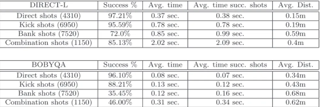
To show the efficiency of the optimization model discussed in this paper, we ran some tests on randomly generated table states and computed possible shots using local and global optimization libraries. We show here only two of the best performers we tested for the sake of brevity. Both approaches were implemented using the NLopt library ([13]). BOBYQA, a local optimization method by Powells [21] was tested with five different starting points, distributed over the possible shot parameters. DIRECT-L, a global optimization method by [14], was tested with only one starting point.
Close to 20,000 various shots were computed using both libraries, to insure a proper sample size. Each of these shots represents a combination of an object-ball, an aimed pocket, a cue-ball and a repositioning target. As can be seen below, types of shots included direct, kick, bank and combine shots.
DIRECT-L Success % Avg. time Avg. time succ. shots Avg. Dist. Direct shots (4310) 97.21% 0.37 sec. 0.38 sec. 0.15m
Kick shots (6950) 95.59% 0.78 sec. 0.78 sec. 0.19m Bank shots (7520) 72.0% 0.85 sec. 0.99 sec. 0.59m Combination shots (1150) 85.13% 2.02 sec. 2.09 sec. 0.4m
BOBYQA Success % Avg. time Avg. time succ. shots Avg. Dist. Direct shots (4310) 96.10% 0.08 sec. 0.07 sec. 0.34m
Kick shots (6950) 88.21% 0.13 sec. 0.12 sec. 0.43m Bank shots (7520) 35.45% 0.12 sec. 0.16 sec. 0.68m Combination shots (1150) 46.00% 0.31 sec. 0.34 sec. 0.62m
Table 1: Results of 19930 different shots computed with the local optimization method BOBYQA and global optimization method DIRECT-L. Average times(seconds) are dis-played for all shots, as well as for successful shots. The average distance (meters) is the distance from the repositioning target.
The local optimization method, even though launched five times with various starting points, gets a slightly lower success percentage for bank and combine shots. The DIRECT-L, however, being a more global approach, achieves better results but at a higher cost in calls to the simulator. What these results actually show us is that we can obtain satisfying results to compute single shots with very few calculations. The trade-off between the solution’s quality and the computation time needs to be carefully studied to achieve the best compromise, but this will also vary with respect to the variant of game played. It should also be noted that in the case a solution is not found for a given shot, it is usually because it is not possible because of other balls or rails restricting the queue motion. Thus a global method may be able to find a solution by doing a spectacular shot, but one that is not very reliable when played on a stochastic system. Further testing is needed to adapt the search criteria to the type of game played, and the level of noise present in the simulator.
5
Perspective
We proposed a description of a new application field, computational billiard. The field is really emerging, and much is to be expected in some near future. However, the ultimate goal to have a computer robot challenge human champions appears quite remote. We did not discuss the robotic aspect of this challenge, but it should be clear that good progress has been made on the computational aspect, and that much remains to be done in this, once again, new field.
From an OR specific point of view, we have described a stochastic dynamic programming framework to model an optimal strategy of a generic billiard player in the presence of noise. The key contribution is an improved estimation of the table value at some stage that takes in consideration the expectation of the difficulty to complete a sequence of winning shots and not only the current one. The present modeling is coherent with the conclusions of Archibald et al [7] who state that ’strategic skill’ is decisive whenever ’the execution skill’ is
imperfect.
On the other hand, we have presented an improved player simulator based on an accurate optimization tool to drive the cue ball trajectory towards the desired spot with the ’best’ table value. Numerical simulations on repeated launching of 8-ball games were performed with relative success, including indirect shots like bank and combine shots, confirming the robustness of our player.
Current work aims at improving the player skill to cope with more realistic situations including the precise modeling of elastic collisions with banks and the breaking of clusters of balls.
Finally, the introduction of defensive strategies to take in consideration the game theoret-ical aspects will be the direction of further studies. It is indeed evident that the development of future competitions between virtual players controlling robots acting on a real table will progressively increase the level of noise effects, thus turning more crucial the improvement of the ’strategic skill’ of the players.
Acknowledgments
We are grateful to Fran¸cois Gaumond and Benoit Hamelin for their careful reading of the manuscript and useful comments and Fran¸cois Gaumond’s work on the Billiards–PoolFiz interface.
References
[1] Classic billard. Canal + multim´edia.
[2] FastFiz. http://www.stanford.edu/group/billiards/FastFiz-0.1.tar.gz. [3] Glossary of cue sports terms. WWW Wikipedia.
[4] David Alciatore. The Illustrated Principles of Pool and Billiards. Sterling, 2004. [5] David G. Alciatore. Pool and billiards physics resources.
http://billiards.colostate.edu/physics.
[6] Christopher Archibald, Alon Altman, and Yoav Shoham. Analysis of a winning com-putational billiards player. In IJCAI’09: Proceedings of the 21st international joint
conference on Artifical intelligence, pages 1377–1382, San Francisco, CA, USA, 2009.
Morgan Kaufmann Publishers Inc.
[7] Christopher Archibald, Alon Altman, and Yoav Shoham. Success, strategy and skill : an experimental study. In Proc. of 9th Int. Conf. on Autonomous Agents and Multiagents
[8] Christopher Archibald and Yoav Shoham. Modelling billiards games. In Sierra Decker, Sichman and Castelfranchi, editors, Proc. of 8th Int. Conf. on Autonomous Agents and
Multiagents Systems (AAMAS 2009), Budapest, 2009.
[9] Gaspard-Gustave Coriolis. Th´eorie math´ematique des effets du jeu de billard. J. Gabay, Paris, France, 1835.
[10] Jean-Michel Fray. Private communication.
[11] Michael Greenspan. UofA wins the pool tournament. Intl. Comp. Gaming Ass. Journal, 28(3):191–193, Sept. 2005.
[12] Michael Greenspan. PickPocket wins pool tournament. Intl. Comp. Gaming Ass.
Jour-nal, 29(3):153–156, Sept. 2006.
[13] Steven G. Johnson. The NLopt nonlinear-optimization package. http://ab-initio.mit.edu/nlopt, 2010.
[14] D. R. Jones, C. D. Perttunen, and B. E. Stuckman. Lipschitzian optimization without the lipschitz constant. Journal of Optimization Theory and Applications, 1993.
[15] Jean-Fran¸cois Landry and Jean-Pierre Dussault. AI optimization of a billiard player.
Journal of Intelligent and Robotic Systems, 50(4):399–417, dec 2007.
[16] Will Leckie and Michael Greenspan. Pool physics simulation by event prediction 1: Motion transitions. Intl. Comp. Gaming Ass. Journal, 28(4):214–222, Dec. 2005. [17] Will Leckie and Michael Greenspan. An event-based pool physics simulator. 11th
Ad-vances in Computer Games: Lecture Notes on Computer Science, (4250):247–262, 2006.
[18] Will Leckie and Michael Greenspan. Pool physics simulation by event prediction 2: Collisions. Intl. Comp. Gaming Ass. Journal, 29(1):24–31, Mar. 2006.
[19] B. M. Miller and J. Bentsman. Optimal control problems in hybrid systems with active singularities. Nonlinear Analysis, 65:999–1017, 2006.
[20] Dimitris Papavasiliou. Billiards. http://www.nongnu.org/billiards.
[21] Michael James David Powell. The BOBYQA algorithm for bound constrained opti-mization without derivatives. Technical report, Department of Applied Mathematics and Theoretical Physics, Cambridge England, 2009.
[22] David S´en´echal. Mouvement d’une boule de billard entre les collisions. Unpublished manuscript, 1999.
[23] Michael Smith. PickPocket: A computer billiards shark. Artif. Intell., 171(16-17):1069– 1091, 2007.